Huybers’ second and more interesting (to me) issue pertains to the benchmarking of the RE statistic.I’m going to start in the middle of this issue. If I start with the history e.g. defining the RE statistic and showing its history (and I just tried), it’s hard to get to the punch line. So what I’m going to do is start with the punch line with minimal history and then go back and put the information into some context.
In our GRL article, having determined that the MBH cross-validation R2 statistic was ~0, we tried to explain the “spuriously” high RE statistic “using “spurious”‘? in the sense of Granger and Newbold [1974] or Phillips [1986]. I’ve posted on some of these articles and, while they were not specifically applied, their viewpoint informs our GRL article and even more in our more recent work.
While the RE statistic may be “preferred”‘? by climatologists [Mann], it has many disadvantags as a statistic. It does not have a theoretical distribution. Its existence has fallen outside the notice of theoretical statisticians and its properties have never been studied from a theoretical point of view. It has however flourished in the world of dendroclimatologists. There we see statements such as the following [Fritts 1991] :
The theoretical distribution of the RE statistic has not been determined adequately so its significance cannot be tested. Any positive value of RE indicates that the regression model, on the average, has some skill and that the reconstruction made with the particular model is of some value.
While dendroclimatologists regularly describe the RE statistic as “rigorous” (and it’s remarkable to see the canonical use of this adjective), one cannot say that the derivation of the statistic is “rigorous”. Anyway, in relfecting on the seeming contradiction between the high RE and low R2 statistics, it seemed quite possible to us that the significance level of the RE statistic has been benchmarked incorrectly in the particular circumstances of MBH98, which, after all, was a “novel”‘? statistical method. Maybe the rules of thumb of regression models as to RE significance did not carry over to this “novel”‘? methodology.
MBH themselves did not merely apply the “rule of thumb”‘? but carried out their own simulations to benchmark RE
Significance levels for ß [RE] were estimated by Monte Carlo simulations, also taking serial correlation into account. Serial correlation is assumed to follow from the null model of AR(1) red noise, and degrees of freedom are estimated based on the lag-one autocorrelation coefficients (r) for the two series being compared. Although the values of r differ from grid-point to grid-point, this variation is relatively small, making it simplest to use the ensemble average values of r over the domain (r < 0.2).
In our GRL article, we pointed out that this benchmarking methodology was inappropriate as it completely failed to emulate actual MBH procedures, where data-mining principal components methods were being applied to much more persistent series. Our view was that the MBH principal components methodology would regularly yield series that had a high RE against NH temperature. If we were re-writing the article today, we would place even more emphasis on the issues and problems of a few “bad apples” with non-climatic trends.
Since we had already shown that the MBH PC methodology yielded hockey stick shaped PC1s, we tested the hypothesis that these simulated PC1s would yield high RE (and near-zero R2 statistics) against NH temperature. This is a different (and we think more subtle) use of the simulated PC1s., than is usually attributed to us. We didn’t say that the MBH reconstruction was simply an artifact of their PC methodology ( a position regularly attributed to us). We’ve always emphasized the interaction between flawed proxies (bristlecones) and flawed methods. But we did say that, if your method was biased toward producing hockey sticks, you would have to treat any hockey stick shaped series resulting from application of this biased method with a great deal of caution. In our RE benchmarking, we applied this insight, by using the biased PC1s to benchmark RE standards. We did not represent this as a complete model of MBH processes (as there were other degrees of freedom in the MBH method that we did not use), but a result obtained only from operations on red noise looked like an excellent way to set a lower limit on RE significance.
We used the simulated PC1s as follows. MBH had fitted proxies to temperature (PCs) by a form of inverse regression (there were other steps as well). So we tried this procedure on the simulated hockey sticks, in our case, by simply doing an inverse regression of the simulated PC1s directly on NH temperature. What were the results? These simulated hockey sticks, generated entirely from red noise, frequently had high RE statistics. In fact, the 99% significance level was 0.59 from our simulations, as compared to 0 in the MBH simulations. Accordingly, as compared with these new benchmarks, the MBH RE statistic (0.47) was high but no longer wildly exceptional. Moreover, the pattern of statistics from these simulated PC1s was completely coherent with the observed pattern – they had high RE statistics, but R2 statistics of ~0. So we felt that we had a pretty convincing explanation of why the MBH RE statistic was spurius.
Enter Huybers. Huybers observed that our predictors (the simulated PC1s) had a significantly lower variance in the calibration period than the target being modeled (temperature). Huybers stated (without any citation) that the adjustment of the variance of the predictor to the target was a “critical step in the procedure”, which we had omitted. Huybers then stated that “when the MM05 algorithm is corrected to include the variance adjustment step and re-run, the estimated RE critical value comes into agreement with the MBH98 estimate [0.0].”‘?
Variance Adjustment
We’ve attempted, without success, to obtain from Huybers a citation as to why he thinks that variance adjustment is a “critical step in the procedure”. GRL would not intervene.
Variance adjustment is a bit of a hot topic in paleoclimate these days. Von Storch et al [2004] attributed the attenuated variance of some multiproxy reconstructions to the use of regression models. (I disagree that this is the correct explanation of the phenomenon of attenuated variance, a feature which I attribute more to a wear-off of cherry-picking effects.) Esper et al. [2005] (et al. including Briffa) contrast results between regression and scaling. Von Storch is hosting a session at AGU in Dec. 2005 in which the topic is mentioned. (I’ve submitted an abstract to this session.)
The argument of Esper et al [2005] is that the predictor should have the same variability as the target. In a regression model, the variability of the predictor is necessarily less than the variability of the estimate, a result familiar to statisticians [e.g. Granger and Newbold, 1973], but a reminder to climatologists was recently issued again by von Storch et al [2004].
If a predictor has less variance than the target, a common naàƒ⮶e response to the desire that the predictor have the same variance as the target is to blow up the variance of the predictor by simply multiplying by the ratio of the standard deviations. Von Storch [1999] here strongly criticizes this approach (citing examples of the discouraged practice back to Karl [1990]), suggesting, as an alternative, adding white or red noise. Granger and Newbold [1973] also discuss this issue, in quite similar terms to von Storch [1999]. I mention this background, because I’m going to come back to these issues after showing some graphs about what happens in the respective simulations and place these results in the context of this debate. I think that the results are very surprising.
MBH98 did not report the use of a variance re-scaling step. However, their recent source code dump (and also the Wahl-Ammann code) shows that they did do a form of re-scaling, but NOT in the method carried out by Huybers. MBH98 took their North American tree ring PC1 and combined it with 21 other proxies in the AD1400 network. They performed a regression-inversion operation (the details of which I’ll describe elsewhere) to obtain a “reconstructed temperature PC1″‘?. They re-scaled the variance of the reconstructed TPC1 to the observed TPC1. This step was added only in April 2005 to Wahl and Ammann code – I mention this to show that the precise existence of this step in MBH was not obvious. From the temperature PCs, they calculated a NH temperature index.
In his Comment, Huybers simply blew up the variance of the simulated PC1s, rather than carrying out MBH98 procedures, which, as it happens, also blow up the variance in the exact degree desired, but in a different way and with completely different results.
We studied the effect using MBH98 methods. Once again, we used the same simulated PC1s from our GRL study. However, this time, we made up proxy networks consisting of one simulated PC1 and 21 white noise series (matching the 22 proxies of the AD1400 network) and did an MBH98 type calculation. Figure 1 shows the before and-after for three PC1s.
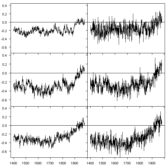
Figure 1. Left (before) – Simulated PC1; Right (after) – “NH reconstruction”‘? using simulated PC1 and 21 white noise series.
On the left is the simulated PC1 fitted against NH temperature (as used in our first GRL calculations) and on the right is the NH temperature resulting from the same PC1 combined with 21 white noise proxy series. It is obvious that the shape and scale of the two series are identical. The biggest observable difference is the increased variance on the right hand side. I hadn’t done graphs in this form at the time when our Huybers response was finalized a few weeks ago, but I find them extremely instructive. While the MBH98 re-scaling operation seems on the surface to be a simple re-scaling of the predictor as criticized in von Storch [1999], the net result is more like an addition of white noise. I’ve always regarded these proxies as operating like noise, but it is remarkable to see exactly what they do in this before-and-after diagram.
The difference between Huybers’ rescaling approach and our implementation of MBH methods is illustrated in Figure 2 below, which should explain the profound differences in RE statistics resulting from the two re-scaling approaches.
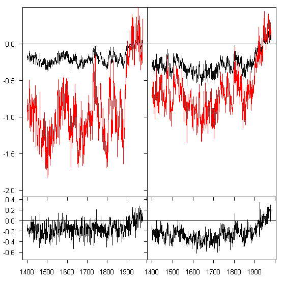
Figure 2. Top: black – simulated PC1; red – recalled according to Huybers’ recipe; Bottom; after MBH methodology, as in Figure 1.
The top panel shows (for two different PC1) the simulated PC1 (black) and the series re-scaled according to Huybers’ recipe. Huybers’ recipe adds variance, but by blowing up the scale of the series. The RE values for the blown-up version (red) are very poor because the scale doesn’t match. It is the act of blowing up the scale that changes the RE performance.
The bottom panel shows the result of adding variance using the MBH method and white noise. (this figure re-states results of Figure 1.) Because the scale is not wrecked in adding variance, the RE properties of the simulated PC1s essentially carry forward into the bottom panel “predictors”‘? which also have high RE statistics against NH temperature, with a critical value also in excess of 0.5. In retrospect, I would probably have done the Huybers’ reply a little differently today than a couple of weeks ago, although the space constraints make it pretty hard to give a detailed reply.
“Real” Proxies versus White Noise
Obvious questions arising from the above is: can you simply model the vaunted MBH98 proxies as white noise? With all the emphasis on persistent red noise in the tree ring networks, shouldn’t you be using red noise?
I’m not saying that I won’t get to a red noise model, but it’s always a good idea to start with white noise and see what adding red-ness does. (I did this with the tree ring PCs as well.) Here we get interesting results simply using white noise. The reason for this may be that we’re in a different stage of the MBH98 procedure: before, we were talking about principal components analysis where the redness made a difference; here we’re doing regression-inversions.
To test the difference between MBH98 proxies and white noise, I tried the following experiments, illustrated in Figure 3 below (see explanation below the figure). I discuss RE results – the “preferred” metric for climatological reconstructions for each panel. As a benchmark, the RE statistic for the MBH98 AD1400 reconstruction (second right) is 0.46, said to be exceptionally significant.
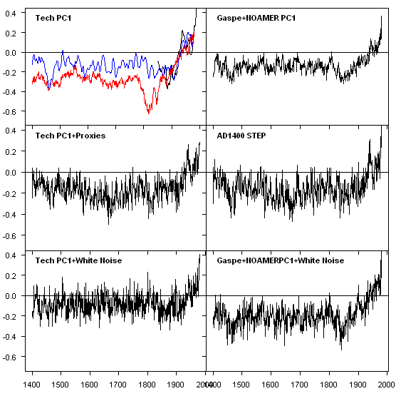
Figure 3. Left – Tech stocks; right – MBH. Top- Tech PC1 and Gasp’-NOAMER PC! blend; Middle ““ plus network of actual proxies; Bottom ““ plus network of white noise.
Some time ago, I posted up the “Tech PC1”, which I obtained by replacing bristlecones with weekly tech stock prices, as an amusing illustration that Preisendorfer significance in a PC analysis did not prove that the PC was a temperature proxy. I re-cycled the Tech PC1 to compare its performance in climate reconstruction against that of the NOAMER PC1 (actually a blend of the NOAMER PC1 and Gasp” – the two “active ingredients” in the 15th century hockeystick.
In the top panels, I fitted both series against NH temperature in a 1902-1980 calibration period. The top right panel shows the Tech PC1 (red), together with MBH (smoothed- blue) and the CRU temperature (smoothed- black). The “Tech PC1” actually a higher RE statistic (0.49) than the MBH98 reconstruction (0.46), but it does have a lower variance (in Huybers’ terms). The Tech PC1 has an RE of 0.49, slightly out-performing both the NOAMER PC1-Gaspé blend (RE: 0.46) and the MBH98 step itself (RE: 0.47). In the most simple-minded spurious significance terms, this should by itself evidence the possibility of spurious RE statistics. Both the Tech PC1 and the Gaspé-NOAMER blend have less variance than the target (and the MBH98 reconstruction itself.)
The second panel show the effect of making up a proxy network with the other MBH98 proxies in the AD1400 network. In both cases, variance is added to the top panel series, in exactly the same way as in the examples with simulated PC1s. The RE for the Tech PC1 is lowered slightly (from 0.49 to 0.46) and remains virtually identical with the RE of the MBH98 reconstruction.
Now for some fun. The third panel shows the effect of using white noise in the network instead of actual MBH proxies. In each case, I did small simulations (100 iterations) to obtain RE distributions. For the “Tech PC1 reconstruction”, the median RE was 0.47 (99% – 0.59), while for the MBH98 case, using the NOAMER-Gaspé blend plus white noise proxies, the median RE was 0.48 (99% – 0.59). Thus, in a majority of runs, the RE statistic improves with the use of white noise instead of actual MBH98 proxies. The addition of variance using white noise is almost exactly identical to the addition of variance using actual MBH98 proxies.
Doubtless, these results can be re-stated more formally. They are hot off the press. At a minimum, the experiment shows the reasonableness of modeling the other 20 proxies as white noise for the purpose of the Reply to Huybers, since there is no evidence that the MBH98 proxies out-perform white noise. (I will on another occasion post up some information about correlations of these “proxies” to gridcell temperature.)
A Digression
This is off topic for the purpose of replying to Huybers, but, since it’s my blog, I guess I can digress. What does all of this mean, aside from merely rebutting Huybers (which is pretty much in hand). These results, which I find remarkable, tell me a lot about what is going on in the underlying structure of MBH98, which was, if you recall, a “novel” statistical methodology. Maybe the “novel” features should have been examined. (Of course, then they’d have had to say what they did.)
When I see the above figures, I am reminded of the following figure from Phillips [1998] , where Phillips observed that you can represent even smooth sine-generated curves by Wiener processes. The representation is not very efficient Phillips’ diagram required 125 Wiener terms to get the representation shown below.

Figure 4. Original Caption: The series f(r)=r^2 on -pi<=r <=pi; extended periodically.
Phillips’ Figure 2 is calculated using 1000 observations and 125 regressors. In the MBH98 regression-inversion step, the period being modeled is only 79 years, using 22 (!) different time series (a ratio of 4), increasing to use even more “proxies” in later periods. My suspicions right now is that the role of the “white noise proxies” in MBH98 works out as being equivalent to a “representation” of the NH temperature curve more or less like Figure 2 from Phillips. The role of the “active ingredients” is distinct and is more like a “classical” spurious regression. I find the combination to be pretty interesting.
Whereas much of my earlier energy was spent just trying to figure out what was done in MBH98. Now I’m thinking about it in more theoretical terms and you can see some of my motivation for wading through the difficulties of Phillips [1998].


61 Comments
Sounds like one heck of a finding!
I’m glad somebody commented on this post. I thought that it might have been my best post so far. It went well beyond replying to Huybers.
The statistical and mathematical interest of what’s going on with this “novel” modeling technique is one reason why I’m drawn back to MBH when, in some sense, I should be dealing with the other multiproxy studies a little more.
It appears to me that the Hockey Stick team knows enough about statistics and statistical analysis to be dangerous. If I understand this post correctly, random data will give the same results as “actual” data in the MBH presentations. If this is true, then isn’t even the data itself suspect?
Or, let’s see if I can ask the questions in a better way… What is the difference between random data and “real” data? And, what types of things would we need to do to discover what the “real” data is telling is? What questions do we need to ask regarding the validity of the “real” data?
It bothers me, that I’ve answered practically every thread of yours including the old ones and not the one that you consider best. Oh well…time to put my dress back on…
You have to allow for the fact that I still have a few math genes in my body and would like to do something mathematical. This probably distorts my appraisals a little. There’s a certain tour de force in comparing the white noise addition in MBH to the Figure 2 representation in Phillips [1998]. I hadn’t figured this out at the time that we submitted our Reply to Huybers and we couldn’t introduce new material in the final version that was not raised in our original submission. So our Reply deals with the narrow issue of RE benchmarking, but doesn’t really explain what’s going on as I’ve done in this post. Although that would have been impossible in the format of a GRL Reply anyway.
Can you publish it somewhere else then? I worry that you are not publishing enough (website is not sufficient) and that when you do, you conflate issues sometimes, rather than carefully disaggregating like a good business consultant should…
I’d like some help from somebody today. I asked Huybers both directly and through GRL to provide a page reference in Rencher [1995] Methods of Multivariate Analysis justifying his (incorrect) claim that standardizing series to common variance was supported by his statistical references. He wouldn’t and GRL did not intervene. In this final version, which I was never sent by GRL, he’s changed the reference to Rencher [2002] 2nd edition and cited page 393. I just noticed this on the week-end. This book is missing from the University of Toronto library. If there’s anyone that has immediate access to Rencher [2002] and can post up or email me any relevant sentences, I’d appreciate it, as I want to contact GRL about it if it makes any difference. I’m a bit pissed at this, especially since we refer to Huybers’ original citation, not the one in his final version.
I’ll definitely try to publish it somewhere. This is a nice discrete little topic. We’ve got a Reply to von Storch at GRL also accepted.
I’ve had a lot of time tied up in these Replies as well as in making responses to 3 other comments. There has been a lot of aftermarket work on our MBH98 articles without touching anything new.
Re #7 ISBN 0471418897. Chapter 12.5 Principal Components from the Correlation Matrix, 393.
The Physics Math Astronomy library at UT Austin has a 2002 copy on the shelf. You might call up the librarian, Molly White (512)495-4610 and ask her to fax chapter 12.5 to you. The call number is QA 278 R45 2002. By the way it is a fantastic library. I worked there back in the card days.
Rencher [2002] problem solved. It came back in at U of Guelph. Page 393, the text is identical with the earlier text.
–after a derivation of PC analysis on the covariance matrix (S)…
12.5 PRINCIPAL COMPONENTS FROM THE CORRELATION MATRIX
Generally, extracting components from S [covaraince] rather than R [correlation] remains closer to the spirit and intent of principal component analysis, especially if the components are to be used in further computations. However in some cases principal components will be more interpretable if R is used. For example if the variances differ widely or if the measurement units are
not commensurable, the components of S will be dominated by the
variables with large variances. The other variables will contribute very little. For a more balanced representation in such cases, components of R may be used.
Huybers uses this to argue that the correlation matix R SHOULD be used and that use of covariance matrix, even in the minor use of our Figure 3, was an error. I’m going to do a whole post on PCs in Huybers. His point is easy to refute. What pisses me off is the extravagant language used by Huybers and both his failure and GRL’s failure to require him to insert more appropriate language. GRL also refused to let us engage in controversy within the article itself, saying that such should be dealt with editorially, which they then didn’t do. I know it’s easy to get paranoid, but there was a real sea change, perhaps after Famiglietti got involved directly.
Agreed, maybe it is a minor error and is irrelevant to the larger issues of the debate and that one can fashion a position for using S rather then R. BUT…if you had to go back to square one, which method is preferable? How much does it change things? If the answer really is that either method could be reasonable used (and the “amount of bias” hinges on this method choice, then there is some reasonable possibility that the lower bias figure of Huybers is correct).
Re #12 To answer your question, for this particular data set, PCs should preferably be taken from the covariance matrix rather than the correlation matrix. The data are prescaled into common, dimensionless indexes and there are no outliers with larger variances. Huybers’ own cited source, Rencher, does not back up the claim that “full normalization” is preferred, and certainly provides no support for his suggestion that we applied a “questionable” normalization. Rencher himself derives PCs using the covariance matrix because that provides the more transparent interpretation of the results. He suggests (2002, pp 383-384) that if you have a data set where 1 variable has a much larger variance than others (because of incommensurable units) it may unduly dominate the results, and in that case using the correlation matrix may be preferable (subject to some caveats on pp. 396-397). But the data set we’re talking about here doesn’t fit that profile. Moreover, we show in the paper why the choice doesn’t actually make much difference, once you get past the graphing trick in Huybers’ article. The overall “amount of bias” in MBH98 results does not trace to the correlation/covariance choice.
Just for the pin down:
So one could do it either way, but yours is slightly preferable? You’re not just defending yourselves legalistically as having made a defensible choice, but you actually think with gun to head, that your way is slightly preferable? (Yes or no)?
(and thanks for clearing up the question as to bias)
We’re not saying that there’s a way to do MBH. Mann said that they used a “conventional” PC calculation. We said, Ok, let’s do a conventional PC calculation and see what happens. There are two somewhat alternate conventions: covariance and correlation. The default PC option is covariance; the texts recommend covariance if you have common units. So we used this to illustrate that Mann’s weird method had an actual impact on a controversial data set. But having identified the impact, we then found that the method mined for bristlecones, which were what was distorting the result. We’re not syaing that covariance PCs are a way of extracting a temperature proxy. That would have to be proven in a special study, if someone wanted to try to do so.
PArt of the problem is that MBH more or less implied that everything that went into his regressions had been pre-qualified by being used a proxy in a peer-reviewed study. THese PC1s were his own concoction and had never been peer reviewed and no one knew what he had done.
Come on. Don’t think of it in terms of “not obscuring the sell recommendation”. Think about it in terms of what Feynman in cargo cult science talks about in terms of analysis of methods and forthrightness about potential issues. I’m not asking for an admission of fault or defense of an action or an in depth independant restudy of Rencher’s advice. I want to know, based on A. your training and mind, B. your reading of methods advice, C. your experience looking at this problem: what your opinion is on the best choice if you are at that decision point in terms of using R or S for this problem. Give me your honest take (not a defense).
As far as “attempting to emulate MBH” based on his written description of methods, yeah…I can see your obvious issues there. Sheesh: look at the acentric normalization method which was not disclosed!
If you have proxies that mainly reflect precipitation with some being fertilized by CO2 and with an average correlation to gridcell temperature of minus 0.08, (with the average reflecting low absolute values, not a mixture of strong positive and strong negative, you would say – go get some better data. You can’t draw any conclusions from this bilge. I’ll post up some histograms to illustrate this in a day or two.
Re #14: “So one could do it either way, but yours is slightly preferable?” Yes, “preferable” in the sense that covariance PCs have a more direct interpretation in terms of the underlying data. I don’t know what I’d say with a gun to my head (probably “Go ask Steve”), but if a student came to me with this data set and said he wants to extract PCs from it I’d say use the covariance matrix. I’d also point out that the computer just pops out lists of numbers: it’s up to the researcher to show what, if anything, they mean.
“Don’t think about it” this way. “Think about it” that way. All in connection with PCA which is not currently within TCO’s grasp.
TCO has gone beyond ditzy. Next stop: the twilight zone.
Twilight Zone, eh? Perhaps that’s why he mentioned R & S in his last message [Rod Serling, get it… hmmm. Why are you looking at me that way?]
Ross: thank you.
Steve: so what if you didn’t know about the CO2 discrepancy or the local grid cell problem (what if you bought into the climate field rationale or were ignorant of the problems with the grid cells) or other questions about the proxies. Which would be the best way to go in the next step in the analysis? (and yes, I agree that this could be different from “what we expect MBH to have done”) When you make comments like you just did, it seems like you are trying to shift from definition of the specific issue. Like saying, “well the balance sheet is all messed up because the equipment list doesn’t reflect reality, so who cares if we use 15 year or 5 year depreciation schedule”. A bad capital equipment list and using the wrong rate for the type of equipment are seperable errors.
Even if you think that either choice is acceptable, I’d like to know which is preferable, for the record. (And even if it is exactly 50-50, or the Huybers method is arguable, then if the choice affects the answer, you have to say that one should consider averaging the two solutions…)
Well, it didn’t take very long for TCO to reach the twilight zone.
Steve, Ross, ignore the actual problems with which you are trying to deal; deal instead with TCO’s ambiguously described alternate world of problems.
Would that constitute contributing to the delinquency of prolific pesterers?
Ok, Jer shut the f*** up and stand the f*** back. I’m ready to dig into this baby. I just reread the Huybers comment (very clearly written by the way) and the MM reply and Steve’s blog posting.
The Huybers text may be slightly overstated, but not that bad. Steve just gets a bit empotional and paranoid and defensive and unable to look at things one by one. The para 2 in MM reply is overly argumentative and strong and actually differs from what he said in the quoted pers comm…”you could use either” as well as being an appeal to authority versus correctness*. Oh…and the Rencher comments are vague and pathetic. Where is the further explication? Where are the proofs. Paf***ingthetic. Hotelling would not be happy with Rencher.
Steve’s comment also centers a bit too much on one little turn of phrase of Huybers rather then his longer explication which is all about emulation of the mean. Oh…and how about the TCO normalization. X(TCO)=X(data). This will match the mean better then any of them…
* I don’t care whether Preisendorfer or Rencher or LaMarche or Fritts or any of them said something. You should be able to defend it now, if it has validity. Otherwise it almost becomes one of those tedious internet arguments which is no longer even about what is right or wrong but about what was alleged in the earlier argument.
I’m reading the RE stuff now, Steve. Pretty darn complicated. Initial impressions:
A. Unfortunate and argumentative that you talk about rsq right at the beginning of the RE section in your formal comment reply. I know that you see this as some sort of “campaign” to malign you, but the fact is that Huybers did not raise rsq as an issue. It is independant. If you really, really have to address rsq because you are worried about the impression people might get (even though H does not say the things you are worried people will think) then talk about it after resolving the actual issues at play in the comment.
B. There is a slew of detail in here that is not in your comment reply. It is probably inappropriate for you to bring these new analyses in given that you did not have room to address them in the reply.
C. And also inappropriate since you never did publish the whole thing.
D. And since, “looking back on it” a few weeks later, you would have changed what you said.
E. I’m trying to read through all this stuff and figure out what is a reasonable method to establish a benchmark for RE and see if either one of you 3 parties ever did it. Given that you never published and elaborated on your rationale, it is frustrating.
I think you read Fritts’s comment the wrong way. He is being very open that the RE statistic is not characterized theoretically. Furthermore, his comment of “some” skill is damning with faint praise. It doesn’t mean 90% confidence.
Perhaps the reason it is a “critical step” has nothing to do with how one should do a temp reconstruction. But has a lot to do with emulating MBH procedure when developing baselines for significance. Essentially it’s the same deal as with off-centering and standard deviation dividing (correlation matrix). It’s not that the correlation matrix is better, but that if you remove off-centering, you are left with the correlation matrix as the comparison, not the covariance.
I don’t have any trouble with anything that Fritts said. Fritts said to look at a variety of statistics. They pretty much assume that a model passes a verification r2 test before they look further.
Mann says that you ONLY need to look at RE. But you can get high RE statistics from nonsense regressions. I got an RE of 0.97 for the damous Yule 1926 nonsense regression between C of E marriages and mortality per 1000. A high RE value is not a guarantee of signficance.
It has virtually no power using power in a statistical sense against a nonsense trend (which is what the issue here is – bristlecone fertilization) or biased selections. Tests which are fine for one thing don’t work against another thing.
The nonclimatic trend thing is a logic flaw, Steve. Get off the CO2 stuff and the dotcom stocks for a second. The issue is mining and bias and significance level. This comes from shape and mathematics of promotion of shapes. What causes the shape is irrelevant. The matrix doesn’t know.
28. Ok. Your impression of Fritts comes across different in context of blog post, but glad to see that we are in agreement. I guess this is why I bother wrestling you down. 🙂
Small note: the high RE of Yule is not such a good example for your general point as it has high R2 as well.
I’m continueing down the post. Now looking at the GRL article, since the post refers to it. In your GRL article, you talk about what Mann does (para 14):
a. Did you replicate Mann’s Monte Carlo simulation? Just to see what he did? THat the numbers work out?
b. you say that 0.2 underestimates the persistence of tree ring series. So what is the correct value?
para 15:
“more closely approximates MBH methods”: why not just duplicate his methods? I think you are criticiszing his bnechmarks (sorry for typose I;’n sringking) for not following his procedure close enough…so why don’t you go all the way and duplicate it, why only approximate it?
15 continued: Interesting comment about the 22 items and the lower limit. Seems to fit into your argument for why you later did use 22 items. out of curiousity, why does more items make the RE calc a lower limit?
16: How fair is the use of PC1s to drive the significance level. Sure within that group, that’s where the 1% falls (above .59=RE). But is that group a relevant test? I’m not arguing btw. Am just trying to think about this. Really, what other types of test runs and protocols have others done with RE in the literature in general? Surely we could learn from that.
para 17. Interesting that even given the tough reassessment that MBH still comes in at 80-90% significance. And when you change from .59 to the lower value from the Comment reply (0.54) that helps MBH even more. So really the whole RE kerfuffle is a bit besides the point, given how good MBH is to start with! I think more rests on the r2 versus RE debate.
I found the white noise versus actual MBH proxies a bit confusing. What with the tech stock PC1 and all. would be better if run with the 1000 PC1s. Also not clear to me if relevant measure is to actual proxies or to red noise (is using the actual proxies a reasonable constraint when benchmarking)?
I could not follow the Phillips/Wiener comments.
Very interesting post (but hard to read, old formatting?).
In calibration, we’ll get smaller (ICE), equal (CVM) or larger (CCE) variance. One figure explains it all http://www.geocities.com/uc_edit/calibration.jpg ICE is based on sampling from normal population, that will be a hard lesson for Storch, Esper et al. That’s what you get when you don’t interact with mainstream statisticians. Incorrect use of ICE causes red residuals, and strong negative correlation between residuals and temperature (just like in MBH9x, hidden ICE there somewhere? ). I haven’t seen a satisfactory theoretical justification for Variance Matching, but maybe I will some day.
Overfitting can happen in multivariate calibration (specially with ICE) 🙂 Maybe that is one reason why Brown writes:
(crossref http://www.climateaudit.org/?p=1681#comment-115322 , still don’t know how one can get white residuals when calibrating noisy proxies with red temperature series)
#38. UC, The quotation and apostrophe signs got screwed up on all old posts when the servers changed. I’ve manually edited this post to tidy it and it should be easier to read now, but I’m hoping someday that John A will figure out how to o this automatically.
#38. UC, one of the interesting undiscussed aspects of variance matching is: what correlation do you need between proxy and target to lower the size of the residuals. The answer is a simple exercise in high school geometry. Regression is obviously the equivalent of dropping a perpendicular. Variance matching is the same as working with isosceles triangles. If you have a correlation of 0.5 – a very high correlation in proxy terms, you have an equilateral triangle, and the norm of the residuals is equal in length to the norm of the signal. The actual expressions are in normed euclidean space, but the high school geometry argument also applies in normed euclidean space.
Having complete faith in McIntyre & McKitrick, I have spent zero time on the issues, thus have not been positioned to appreciate Steve’s work in this post (sorry bout that). But from listening to the words, part of what is going on seems to arise from nature of the underlying distributions going into the PC analysis. For completeness I would note that the ultimate distribution levelizer is to run the PC analysis in rank order space. Interactions that survive this treatment are usually not artifacts of lumps in the primary distributions.
#41. The bristlecones are a real thing in the data. The question is whether their 20th century growth has anything to do with temperature.
Hmm, lower the size compared to what? Let’s see,
Correlation of 0.5 means 60 degrees between Pc and Tc (calibration proxy data and calibration temperature data), OK, equilateral triangle in the CVM case 🙂 And calibration residuals (dashed in the figure) are bounded by temperature data, just like in ICE. Only CCE allows very large calibration residuals. That’s why it is not very famous in proxy studies ( Juckes INVR is essentially CCE, but he didn’t report 2X calibration residuals for that case, because it is illegal to make CIs exceed modern temperature record)
RE 42: Is there a reason why the conventional rank correlations won’t work, assuming interpolation to a consistent time base?
If the variables need to be unraveled with a PC analysis, the front end transform to rank is not difficult, is it?
Transforming to rank does not destroy information, but does make the significance tests much less ambiguous because the distributions are now known to be rectangular. (I’ll bet $5 to the tip jar that none of the input distributions are even remotely Gaussian.)
Hint: I have absolutely no idea what UC said in 43.
#44. Allan, you’re missing the point of this post. It’s not about PC analysis. It’s about spurious regression in a multivariate situation that hasn’t been discussed in any literature to my knowledge.
#43. UC, I posed a related puzzle last year http://www.climateaudit.org/?p=731 which no one answered. I think that it’s amusing that all this huffing and puffing can be equated to high school (really grade school geometry).
To others, in linear algebra, there is an intimate relation between inner products, correlations and cosines. IF you think about correlations as an angle ( a point of view in my ancient textbook, Greub, Linear Algebra; standard deviations are a norm (“length”) from an inner-product space point of view; thus you can use simple high school geometry diagrams to understand what’s going on.
Think of the signal as a line segment in one direction and the proxy as a line segment in another direction, both through the origin. The regression best-fit is the line segment from the origin to the foot of the perpendicular from the signal to the proxy and the error is the length of the perpendicular. The length of the perpendicular is always going to be less or equal to than the length of the signal line segment by simple geometry (equal to only in the case of the proxy being uncorrelated = perpendicular to the signal). These sorts of perpendicularity/orthogonal arguments underpin the entire linear regression apparatus.
But in CVM, you have a different, but also simple geometry, but one which people haven’t thought about in the same way. Because of tghe variance equalization step, you have to think of two line segments with the same length both from the same origin. The length of the residuals (standard error) is the length of the line segment from the signal to the proxy. If the angle between the segments is greater than 60 degrees (equivalent to a correlation less than 0.5 since correlation = cosine of the angle), then the standard error is greater than the standard deviation of the signal and you have a negative RE. RE in this context is equivalent to the cot instead of the cos.
When you have a different verification period, you have to consider a situation in which origins can differ.
Let me try,
Use the ICE triangle in #43, RE is , where Res is the orange dashed line. r is the cosine of the angle between Tc and ICE. ICE triangle is a right triangle, hence r equals ICE / Tc (adjacent / hypotenuse ). Next you’ll need Pythagorean Theorem,
  . Square r and you’ll have
Use the CVM triangle of #43, r is the cosine of the angle between Tc and CVM. Tc and CVM are equal length, apply the law of cosines and you’ll get
re-arrange a bit and you’ll see that
and thus
And as you said, high-school geometry can be generalized to N-dimensional space.
Quite so. I thought that it was rather a pretty result – one that is obviously unknown in the literature and one which illustrates how the statistic work rather well by de-mystifying them. It shows the need for people advocating CVM as some kind of a magic bullet to think a little about what they are doing.
Yes, properties of those rigorous statistics are very interesting 😉
..and here’s another thing that I find hard to explain with white reconstruction errors:
MBH98 full network vs. calibration temp (1902-1980) r^2 = 0.7587
MBH98 full network vs. sparse calibration temp (1902-1980) r^2 = 0.5343
MBH98 full network vs. verification temp (1854-1901) r^2 = 0.0596
MBH99 AD1000 step vs. calibration temp (1902-1980) r^2 = 0.4024
MBH99 AD1000 step vs. sparse calibration temp (1902-1980) r^2 = 0.1783
MBH99 AD1000 step vs. verification temp (1854-1901) r^2 = 0.0014
Did I compute these correctly?
(Dr. Rutherford, pl. redraw Figure S1 in miscsupp.pdf with white errors and red temperature ..)
#49. The errors in the reconstructions are not white. I presented Durbin-Watson statistics on all the canonical reconstructions at AGU a couple of years ago. The pattern is a failed DW in the calibration period and a failed verification r2 in the verification period.
There’s a very interesting type of noise that I looked at a couple of years ago – “near white, near integrated”. Perron has discussed it in econometrics. For example, if you have a high AR1 coefficient say more than 0.9 accompanied with high negative MA1 coefficient. It’s hard to make tests against this – and, unfortunately, an ARMA(1,1) fits temperature data and other series much better than AR1. (Koutsoyannis has also shown that AR1 is not a sensible model when you include averaging and averaging occurs in all climate data, months, years, etc.)
Anyway back to MBH, he blends some white noise into his reconstruction by overfitting, and I think that’s what gets his DW onside. The low-frequency portion which is driven by bristlecones has hugely red residuals.
#49. UC, what did you use for the MBH99 AD1000 step? Did you use your emulation?
And the you got a standing O from the Team? 🙂
Yes. Some other correlations that are worth checking:
MBH full residuals vs. dense temperature (1902-1980) r = -0.3820
MBH AD1000 residuals vs. dense temperature (1902-1980) r = -0.4706
MBH AD1000 residuals vs. sparse temperature (1902-1980) r = -0.8006
re: 45 Steve: I am doing a dreadful job of communicating, or worse yet, not. At the risk of total alienation, I forge forward. You can always delete it. Years ago the key to solving a set of related manufacturing problems that had stopped a small army of engineers and scientists in two fortune 500 companies was nonparametrics. Since then, I have had the opportunity to try nonparametrics in parallel with parametrics many times, and if there was a difference, the nonparametric result was the one which subsequently verified — always. I do not mean just correlations, but multivariate interactions of laboratory and process variables and process tuning based on customer feedback. I grant that ultimately one must move back into parametric space (J.Qual.Tech. V29, 1997, pp 339-346), but the first problem is to isolate the critical variables from the noise.
Nonparametrics work well with chaotic data. Because you do not change the distributions, just the significance level, you can strip chunks out of data, i.e., top half, mid quartile, etc, that would be unthinkable in parametric statistics. So my need is to go with nonparametrics, the more so if there is a question on the significance of a parametric relation between data sets, and it does appear that you have several questions. Heaven only knows where a nonP replay would leave the hockey stick, but having watched many people stumble with their hand calculators and built in R(Pearson) I’m not a believer until I hear at least R(Spearman).
A P/nonP example is as follows. In Fisher’s book “The Design of Experiments” (1971 reprint) he runs his t test on Mr. Darwin’s Zea Mays(young plants). He concludes that there is a (barely) significant difference between “crossed” and “self fertilized”, @ 5% supporting Mr. Darwin over Mr. Galton, a triumph of t over Galton. But the Smirnov two sided on the same data show highly significant difference @ 1%. (While accurate, this story is far from complete, so it is worth tracking a copy down.)
The situation is quite funny. Essentially ICE is based on assumption of stationarity, i.e. calibration temperatures are representative sample of past temperatures (no AGW). VS04 notes that if you use ICE, you’ll underestimate past temperatures (if they exceed the calibration data range). Mann responds to criticism by claiming that VS04 ‘simulation was forced with unusually large changes in natural radiative forcing in past climates’. IOW, it is ok to use ICE-like estimators because past temperatures were in the range of calibration temperatures. And these high-school kids are in power..
Something related:
(Mann et al 2005, Testing the Fidelity of Methods Used in Proxy-Based Reconstructions of Past Climate, my emph).
I wrote this ICE vs. CCE and associated CI stuff a bit more formally here:
http://signals.auditblogs.com/2007/07/05/multivariate-calibration/
Profs. Brown, Sundberg etc. probably will tell me where I go wrong with this, I’ll let you know 🙂
I suspect that there is some circular logic here. Steve says that what he is using is “just red noise”, but it has MANY parameters to it (a lot of fitting). It’s NOT a simple AR1 or (1,1) model. And it is based itself off of the bcps which at least are in question as to whether there is a century scale signal.
This is maybe the most interesting thread here, it is good to bring it up from time to time. However, I don’t quite understand your comment, where’s the circular logic? Where’s the fitting?
Note Mann’s comment in #54. ICE or CPS + CIs from calibration residuals = upper-bounded errors, before seeing the data (remember Juckes and CVM). Not completely unlike a civil engineer who is about to design a bridge, and tells you the weight limit before choosing the material.
(Caveat) First, it’s not an allegation. It’s something I want to check.
a. My understanding is that Steve made his “just red noise” proxies by taking the acf of each of 70 specific proxies used in the actual study. The acf has 5+ parameters to it. That’s 350 parameters. Now maybe some are irrelevant. But still it worries me as a possible problem. The “just red noise” not being some simple set of duplicated AR1 or 11 proxies. They are highly modeled noise derived from the actual sample set.
b. In addition, the actual sample proxies were not detrended, yet there is at least an open question as to whether there is a meaningful signal within those proxies. Thus some aspects of signal (or at least debated, open to question) signal are being a priori defined as noise.
OK, Steve’s red noise is probably , where x is i.i.d zero mean unity std Gaussian vector. And you are afraid that
  carries information to that noise, as it is estimated from the proxies. Sounds a bit far-fetched, but should be easy to check. Just force
  to a covariance matrix of AR1 process, and re-run.
Of course there is some meaningful signal in the proxies, trees don’t grow at all if temperature is 400 C, or -150 C. Other aspects of your part b remain unclear to me. But I Know I need to study MBH98 methods (and Steve’s articles) more. (Still kind of stuck to the evolving multivariate regression part.)
But the issue is that he did not just use a simple AR1 or AR11 method. He used a method that extracts the noise from a record and creates new series based on it. How do we then know that all of what he extracted is really noise? Is it relevant to call it “just noise” if it has so much connection to the actual experimental evidence? (This is the circular logic I’m concerned about.) I will bump the thread (read the comments) where we finally got a better hand on what Steve was doing with his noise generation. You actually have to go to code 9including a subroutine) to understand it.
Link: http://www.climateaudit.org/?p=836#comment-124625
2 Trackbacks
[…] that they assert using either CPS or Mannian methods. The graphic below, taken from a CA post here from a few years ago shows the impact of replacing all the “proxy” series in the MBH98 […]
[…] me by Eduardo Zorita) and one using pseudoproxy networks constructed to emulate the MBH98 network (Huybers #2 and Reply to Huybers) also here and I’ll try to tie these three different studies […]