MBH Calibration-Estimation Procedure

What I’m going to show here is that the MBH98 method can be reduced to a few lines of code and, in doing so, show some other interesting results as well. Today I’m just going to get to the reconstructed temperature PCs, but I’ll show that these are linear in the proxies and later show that the NH temperature index is, up to a very slight linearization in the RPC re-scaling step, also linear in the proxies. We reported this as long ago as MM03, but I’ve never shown this in detail. The result is important because it contradicts claims by MBH, von Storch et al [2004] and Zorita et al [2003] that the effect of individual proxies cannot be isolated. I’ve been massaging this material for a long time and plan to submit it for publication. Recently, Mann has argued that RegEM is a magic bullet and I’ve been re-visiting my methodological notes.

In the important case where only one temperature eigenvector is reconstructed (the AD1400 step in MBH98 and the 1000-1399 step in MBH99), I’ll show that the weights assigned to each proxy are proportional to the correlation of each proxy to the temperature PC1 – demonstrating the essential similarity of MBH98 methodology to “correlation weighted” proxies used in other studies [e.g. Mann and Jones, 2003].

The procedure described here (or close variations up to re-scaling) has been used since MM03. I have reconciled all results step by step to Ammann and Wahl source code (discussed last May) and have analysed MBH98 source code. I’ll discuss some nuances pertaining to weighted regression in the next instalment. (I apologize for transpose where you’ll have to read T as a transpose, as I can’t figure out how to do a superscript on “WordPress”).

MBH98 has 11 steps with the first step beginning in AD1400 with 22 proxies and 1 reconstructed temperature PC (RPC) and the last step beginning in AD1820 with 112 proxies and 11 RPCs. Note that the temperature PCs are different than the tree ring PCs and were obtained by a PC decomposition of 1082 gridcell series interpolated so that there were no missing values. For the analysis here, the steps don’t matter, although I will discuss separately a simplification resulting from use of only 1 RPC.

Calibration
MBH98 stated that they “trained” the proxies by finding the “least-squares optimal combination” of (temperature) PCs to represent the proxies. Their procedure is described in typically rotund and inflated prose as follows:

These Neofs eigenvectors were trained against the Nproxy indicators, by finding the least-squares optimal combination of the Neofs PCs represented by each individual proxy indicator during the N=79 year training interval from 1902 to 1980 (the training interval is terminated at 1980 because many of the proxy series terminate at or shortly after 1980). The proxy series and PCs were formed into anomalies relative to the same 1902-80 reference period mean, and the proxy series were also normalized by their standard deviations during that period. This proxy-by-proxy calibration is well posed (that is, a unique optimal solution exists) as long as N> Neofs (a limit never approached in this study) and can be expressed as the least-squares solution to the overdetermined matrix equation, Ug = Y[,i] , where U is the matrix of annual PCs, and Y[,i] is the time series vector for proxy record i. The Neofs-length solution vector g = G[i,] is obtained by solving the above overdetermined optimization problem by singular value decomposition for each proxy record i = 1,…,Nproxy. This yields a matrix of coefficients relating the different proxies to their closest linear combination of the Neofs PCs .This set of coefficients will not provide a single consistent solution, but rather represents an overdetermined relationship between the optimal weights on each on the Neofs PCs and the multiproxy network. [ notation slightly re-stated for consistency with notation here.]

The most obvious implementation of the above procedure is qr-minimization, which for the i-th proxy yields a Neofs -length vector of coefficients G[,i] as follows:

1) $G[,i] = qr.solve( U, Y[,i] )$ , for i = 1,…, Nproxy

where G is the matrix of calibration coefficients, U is the matrix of (selected) temperature PCs and Y is the matrix of proxies, with both U and Y restricted to the calibration period cal. (The index cal restricting the matrices to the calibration period will be assumed but not shown in these equations, but is in all code where appropriate. The indexing in equation (1) is according to the conventions of S and R.) This is the approach used in Ammann and Wahl code (which like ours is in R).

The above procedure can be seen to be no more and no less than a multiple linear regression of each proxy in the calibration period against Neofs temperature PCs (TPCs) without a constant term:

2) $Y[,i]$ ~ $U[,1] + U[,2] +$ … $+U[,Neofs]$ for i=1,…, Nproxy

In the formalism of R,

3) G[,i] = lm( Y[,i] ~ U -1) )$coef

The coefficients from regression and from qr-minimization are identical. An important advantage of recognizing the inherent regression nature of the calculation is that there is considerable literature on statistical significance in regression. The regression formalism of equation (6) enables the calibration procedures to be viewed in more general statistical terms, enabling the consideration of the validity of individual statistical relationships through t-statistics, Durbin-Watson statistics. Merely expressing the problem in qr-minimization terms does not avoid the need to consider statistical significance. While it is beyond the scope of this note, many of the key individual calibrations (e.g. Gaspé tree rings) fail standard regression diagnostics testing for mis-specified or spurious relationships.

The matrices of regression coefficients G, which have dimension Neofs by Nproxy, can be rather large. In the 1820 step, there are 11×112 coefficients and 1×22 coefficients in the AD1400 step. Each linear regression can be expressed as:

4) $Y[,i]= U * G[,i]+ \epsilon [,i]$ , for i = 1,…, Nproxy,

the stacked version of which is:

5) $Y= U * G+ \epsilon$

Regression assumptions presume independent identically distributed (i..i.d) errors, which is not demonstrated in MBH98 and appears to be untrue, although this discussion is beyond the scope of this article. Standard linear algebra solves for the coefficients G as follows:

6) $G = (U^T * U)^{-1} *U^T *Y$

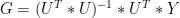
We use this formula in our code, which in one line yields all the calibration coefficients for a single step. Again we emphasize that results reconcile exactly from this step to both Ammann and Wahl code and MBH98 code mutatis mutandi.

Although MBH did not report many salient details of their calculations, here they reported that used singular value decomposition to obtain their calibration coefficients. Indeed, instead of calculating the matrix G directly as above, it is possible to derive identical results using principal components, which can be shown as follows. First, Mann carried out a PC decomposition [UU,SS,VV] of the matrix U of temperature PCs, yielding:

7) $UU * diag( SS) * VV^T = U$

They then calculated the matrix of coefficients G through a series of operations in Fortran equivalent to the following formalism ( a transliteration of their Fortran steps is here):

8 ) $G = VV^T * diag(1/SS) * UU * Y$

This formalism yields identical results in the unweighted step as the usual regression linear algebra as shown here […], but problems arise in the weighted case as discussed here [].

In the AD1400 step (and the AD1000 step of MBH99), MBH only use one temperature PC (U[,1]) in the reconstruction. This changes the matrix formulations into vector formulations and enables some helpful simplifications. The covariance between a TPC and the i-th proxy (and mutatis mutandi, variances) can be expressed in inner product terms as follows:

9) $cov(U[,1],Y[,i]) = (N-1) * {U[,1], Y[,i]} = (N-1) * U[,1]^T * Y[,i]$

Accordingly, a regression coefficient in equation (6) can be expressed as follows:

10) $G[1,i] = (U[,1] * U[,1] )^{-1} * {U[,1], Y[,i]}= \frac{cov(U[,1],Y[,i])} {var (U[,1])}$

If the vector G[1,] is denoted by $\gamma$ and applying cov and sd to the columns, then we get:

11) $\gamma = \frac {cov (U[,1],Y)} {var(U[,1])} = cor(U[,1],Y) * \frac{sd(Y)}{sd(U[,1])} = \frac{cor (U[,1],Y)} {sd(U[,1])}$

since the proxies Y are standardized in the calibration period. In other words, the calibration coefficients àÅ½àⱠfor the AD1400 step are proportional to the individual correlations of each proxy to the TPC1. (This would apply, mutatis mutandi, for the TPC2,…)

Estimation of RPCs
The estimation step in MBH98 consists of the estimation of the matrix $\hat{U}$ of reconstructed TPCs, a step once again described in MBH98 in rotund prose as least-squares minimization.

Proxy-reconstructed patterns are thus obtained during the pre-calibration interval by the year-by-year solution of the overdetermined matrix equation, Gz = y [j,], where y[j,] is the predictor vector of values of each of the P proxy indicators during year j. The predictand solution vector z= $\hat{U}$ [j,] contains the least-squares optimal values of each of the Neofs PCs for a given year. This optimization is overdetermined (and thus well constrained) as long as P >Neofs which is always realized in this study. It is noteworthy that, unlike conventional palaeoclimate transfer function approaches, there is no specific relationship between a given proxy indicator and a given predictand (that is, reconstructed PC). Instead, the best common choice of values for the small number of Neofs predictands is determined from the mutual information present in the multiproxy network during any given year. The reconstruction approach is thus relatively resistant to errors or biases specific to any small number of indicators during a given year. This yearly reconstruction process leads to annual sequences of the optimal reconstructions of the retained PCs, which we term the reconstructed principal components or RPCs and denote by $\hat{U}$ [,k]. [notation changed slightly]

Again, the most obvious implementation of the stated procedure is through qr-minimization (this time on a year-by-year basis), which yields for the reconstruction of the k-th temperature PC in the j-th year:

12) $\hat{U} [j,k] = qr.solve(G[k,], Y[j,] )$

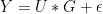
Once again, this is the procedure applied by Wahl and Ammann. Once again, this is formally equivalent to a linear regression without an intercept – this time, the proxies are regressed against the calibration coefficients, being expressed as follows:

13) Y[j,] ~ G[k,1] + G[k,2]+ … +G[k,Nproxy], for j=1,…, Nyear; for k=1,…,Neofs

In the AD1820 step covering 161 years, there are 11×161 regressions yielding 11×161 individual RPC values. Equation (13) can be interpreted as:

14) $Y[j,]= U[j,] * G+ \epsilon [j,]$ , for j = 1,…, Nyear,

or stacked (this time estimating U instead of G):

15) $Y = U * G + \epsilon$ ,

The direct linear algebra solution of the qr-minimization (or the regression) is the following:

16) $\hat{U} = Y * G^T * ( G * G^T)^{-1}$

The stacking is very awkwardly handled in the Ammann and Wahl code, where the calibration and pre-calibration periods are handled separately, although the matrix algebra is identical and the stacking yields identical results.

Once again, Mann source code shows that they carried out operations which yield identical results to equation (16) in an unweighted case using PCA methods, similar to the corresponding operations used for calibration. Once again, temporarily leaving aside weighting issues, MBH98 first carried out PCA on the transpose of the matrix of calibration coefficients $G^T$ , yielding the triplet [UUU,SSS,VVV] such that:

17) $G^T = UUU * diag( SSS) * VVV^T$

They estimated the matrix $\hat{A}$ of reconstructed temperature PCs as follows:

18) $\hat{U} = Y * UUU * diag(1/SSS) * VVV^T$

All derivations of $\hat{U}$ in unweighted cases yield identical results. Using direct linear algebra, all the reconstructed PC series $\hat{U}$ in MBH98 can therefore be derived in 2 lines:

$G = (U^T * U)^{-1} *U^T *Y[503:581,]$
$\hat{U} = Y * G^T * ( G * G^T)^{-1}$

In the case where only one TPC is used in the reconstruction, we have from (11): $\gamma= cor (U[,1],Y)/sd(U[,1])$ where cor (U[,1],Y) is the columnwise correlation of the PC1 U[,1] with the standardized proxies Y. Denote this vector by $\rho$ and let u = U[,1].

Simplifying equation (16) in this case:

19) $\hat{U}= Y * G^T * ( G * G^T)^{-1} = Y * \gamma^T * ( \gamma * \gamma ^T)^{-1}$
$\hat{U}= Y * \rho^T * sd(u)^{-1} (\rho^T * sd(u)^{-1} *sd(u)^{-1} * \rho) ^{-1}$
$\hat{U}= Y * \rho^T *sd(u) * (\rho^T * \rho ) ^{-1}$

That is, the reconstructed TPC1 in the AD1000 and AD1400 steps is simply a linear weighting of the proxies, with the weights proportional to their correlation $\rho$ to the TPC1.

The final RPC includes a re-scaling step described in the following post on this topic here.

Tomorrow I’ll talk about calculating the NH temperature reconstruction in one more line of code. See continuation here.

This entry was written by Stephen McIntyre, posted on Feb 6, 2006 at 10:46 AM, filed under MBH98, Replication, Source Code and tagged algebra, linear algebra. Bookmark the permalink. Follow any comments here with the RSS feed for this post. Both comments and trackbacks are currently closed.

47 Comments

Armand MacMurray

Posted Feb 6, 2006 at 12:30 PM | Permalink

It’s pages like this that really make ClimateAudit rise above the other sites. Now to start boning up on R…
John S

Posted Feb 6, 2006 at 2:20 PM | Permalink

When I worked through their prose and came up with the utterly familiar beta=inv(x’x)*(x’y) I was less than impressed.

People may have cared about computational methods for matrix inversion (i.e. SVD) decades ago – but these days you have to ask yourself why they bother.
John A

Posted Feb 6, 2006 at 2:58 PM | Permalink

Steve,

Mann’s prolix statement:

Instead, the best common choice of values for the small number of Neofs predictands is determined from the mutual information present in the multiproxy network during any given year. The reconstruction approach is thus relatively resistant to errors or biases specific to any small number of indicators during a given year.

As I understand it, they had one proxy for the early 15th Century, which in the earliest decade-and-a-bit consisted of exactly one tree (the famous lone Gaspé cedar). What the hell are they talking about?
fFreddy

Posted Feb 6, 2006 at 4:27 PM | Permalink

Come to think of it, who were the reviewers for MBH98 ? And what are they reviewing now ?
Spence_UK

Posted Feb 6, 2006 at 5:47 PM | Permalink

This might make me sound like a nerd, but it is a good feeling to work your way through a raft of messy equations and end up with something so simple and elegant.

Nice work, Steve.
Louis Hissink

Posted Feb 6, 2006 at 6:24 PM | Permalink

“Simplify Simply”, Thoreau I believe.
Brooks Hurd

Posted Feb 6, 2006 at 6:28 PM | Permalink

Steve
To get a superscript, the html code is “sup”. You would make eT with e””T”” with the quotation marks removed.
A subscript uses “sub” H2O
Brooks Hurd

Posted Feb 6, 2006 at 6:28 PM | Permalink

Drat!
It works in the preview, but not in the submission.
Steve McIntyre

Posted Feb 6, 2006 at 10:52 PM | Permalink

The silly thing is that there is nothing in this analysis that is beyond the skills of a capable sophomore or even freshman. In my next post on this, I’ll show the linear relation between the NH index and the proxies. While the math is easy, it eluded von Storch and Zorita. For example, Zorita et al [2003] stated:

MBH98’s method yields an estimation of the value of the temperature PCs that is optimal for the set of climate indicators as a whole, so that the estimations of individual PCs cannot be traced back to a particular subset of indicators or to an individual climate indicator. This reconstruction method offers the advantage that possible errors in particular indicators are not critical, since the signal is extracted from all the indicators simultaneously.”

Von Storch et al [2004] stated:

The optimized temperature fields target the whole available proxy network at a given time, so that the inclusion of a few instrumental data sets in the network should have little influence on the estimated fields, unless the instrumental records are explicitly overweighted. The advantage is that the method is robust against very noisy local records. This contrasts with direct regression methods, where the estimated temperature fields are the predictands of a regression equation. In this case a few instrumental records, highly correlated to the temperature fields, may overwhelm the influence of proxy records with lower correlations in the calibration period.”

So even though this analysis is pretty simple, the other guys grabbed the wrong end of the stick, so to speak.
john

Posted Feb 7, 2006 at 12:12 PM | Permalink

Can someone point me to the data? Thanks.
john

Posted Feb 7, 2006 at 12:44 PM | Permalink

Maybe this blog is not the right place to put this, but a list of links (somewhere) pointing to the various data sources would be really useful for hobbyists like myself (I’m a physicist, but my work has nothing remotely to do with climatology, I am not up on the papers, etc.) I’m sure I could dig through the Web, go through papers, etc. and find the sources, but if someone knows where an existing collation of the datasource links is already that would be great.
Steve McIntyre

Posted Feb 7, 2006 at 4:17 PM | Permalink

The current version of Mann’s data is at the Nature SI:
http://www.nature.com/nature/journal/v430/n6995/suppinfo/nature02478.html

Also check out Mann’s FTP site – ftp://holocene.evsc.virginia.edu/pub/MBH98 (I’m not sure whether this is still live): I tried using a web disguise and it doesn’t seem to be up any more. He’s moved his publications to Penn State, but doesn’t seem to have moved his data into a public access point.

I’ve posted up pdf’s for many multiproxy studies at http://www.climateaudit.org/pdf . I’ve collated data versions for most of the multiproxy studies where possible and will post that up. Actually, it would be amusing to post up a sticky with an inventory of what’s missing and I’ll try to do that some time as well.
Armand MacMurray

Posted Feb 7, 2006 at 5:05 PM | Permalink

Re:#12
Your disguise must not have fooled them – the holocene site is visible to mere civilians like me.
Pat Frank

Posted Feb 7, 2006 at 5:33 PM | Permalink

#13&12 — Yup, it’s there for me, too. That orange wig must not have fooled them, Steve. 🙂
john

Posted Feb 8, 2006 at 11:14 AM | Permalink

Thank you for the data links. Looking at it now.

Just as an aside, I was thinking about the similarity of using tree rings as a proxy for temperature to using individual stock prices as a proxy for economic output (or worse, individual stocks from several different countries to gauge global output). This made me think about the practical difficulty in linking the two in a quantitative way (normalizing to externally measured values seems dangerously like circular logic). Qualitative, yes of course and if one is just looking for the existence of bumps or dips then fine no problem, quantitative, at the moment I don’t see how to do it in anyway that isn’t seriously flawed.
Steve McIntyre

Posted Feb 8, 2006 at 12:39 PM | Permalink

#15 – the stock price perspective is a very useful one. One of the differences in my approach to data and Hockey Team approach to data – and I’m just gradually focusing on this difference – is that I come at data from a stock market perspective – I don’t believe in stock market “systems”, one sees various studies that hypothesize that various indicators are linked to stock market performance and they always fail out-of-sample. Ferson has pointed out how data mining methods will pick out highly autocorrelated series which give calibration-period overfitting. The starting point for me with proxies is – show me and not by data mining. The Hockey Team all start with “signal-noise” concepts, which are not what stock market pickers think about. They declare that various time series are “proxies” and then try to extract the “signal” from the “noise” without paying any attention to biases in the series selection etc. I don’t think that they even realize some of the places where they are simply arm-waving through problems, even though the arm-waving is obvious to someone with stock market background.
Phil B.

Posted Feb 11, 2006 at 11:02 AM | Permalink

Steve, I know you’re busy but are you going to present this “Tomorrow I’ll talk about calculating the NH temperature reconstruction in one more line of code.” Or did I miss it thanks Phil
Steve McIntyre

Posted Feb 11, 2006 at 6:59 PM | Permalink

Phil, I’ll get to that. I got involved with responding to O&B, which was topical
TCO

Posted Jun 22, 2006 at 8:01 AM | Permalink

I’m interested in the brief comment about regression relying on iid and that Mann’s inputs are not iid. How un-iid are they? And how much does this affect regression?
fFreddy

Posted Jun 22, 2006 at 8:57 AM | Permalink

Re #19, TCO
Look at the posts on ARMA processes. You might like to put your “the market has no memory” conditioning to one side …
TCO

Posted Jun 22, 2006 at 9:30 AM | Permalink

I’ve read the whole site, Fred.
UC

Posted Aug 7, 2007 at 4:17 AM | Permalink

Not sure where is the most appropriate thread, but I’ll write here.

As I promised to TCO, http://www.climateaudit.org/?p=370#comment-124617 , I started studying Mann’s PC methods. At this point, I managed to reconstruct MBH99 AD1000 step using Mann’s data (1), Steve’s blog (2,3), and JeanS’ advice. Result agrees very well with reverse-engineered AD1000 step ( p=0.999999948; 2*std = 0.002 C), and with those scanned residuals (4).

Some comments (Matlab code will be available soon, need to upload those mat-files to web first..)

a) Mann does almost conventional multivariate CCE with proxy data, but the reference in the training is TPC1. CCE outputs always a series with a larger variance than the target. Thus, the variance of reconstructed PC1 is larger than the original. But see Mann’s code,

c insure that reconstructed pcs are properly
c normalized (amplitude determined by fraction
c of calibration resolved variance of actual pc)

This means that reconstructed PC is standardized to unity (cal period) and then multiplied by std of target PC and finally by the correlation of target and reconstruction. This scales the reconstruction down, guarantees that reconstruction variance is always less than the instrumental temperature. Keeps the uncertainties upper-bounded, whatever you put in.

b) Steve is right, Mann’s method overfits and makes hockey sticks from red noise data. Partially it is due to CCE, but if Mann would use CCE without any PCA and scaling tricks, there would be no hockey stick as we know it know:

Refs:
1 http://holocene.meteo.psu.edu/shared/research/MANNETAL98/INSTRUMENTAL/
2 http://www.climateaudit.org/
3 http://data.climateaudit.org/data/MBH99/
4 http://www.climateaudit.org/?p=647
TCO

Posted Aug 7, 2007 at 9:06 AM | Permalink

I’m not sure how this relates to what I asked about (Steve M’s method for benchmarking RE, using red noise, whose characteristics were dependant on the actual sample set (and if that was circular logic)).
UC

Posted Aug 7, 2007 at 12:06 PM | Permalink

TCO, IMO now the burden of proof is now on Mann’s side, he’s the one who uses novel statistical methods.. Anyway, #22 is not directly related to your question, but might be useful if you prefer Matlab over R (like I do). Here’s the code:

http://signals.auditblogs.com/files/2007/08/mbh99.txt

You’ll need to download and rename few files, but that’s all. After that you’ll be able to reconstruct that famous AD1000 step of MBH99 with Matlab. And then you can test different noise models easily.
TCO

Posted Aug 7, 2007 at 1:10 PM | Permalink

Maybe so, but then your response does nothing to allay my question and just means that I need to do the work myself. Otherwise, I just need to keep that caveat/caution about Steve’s work.

BTW, from your reaction to my comments, it does not seem clear to me that you understand where I have questions or that you remember some of the discussions here. I would also add that the last couple pages of Burger are very useful persepctive on the area of interest to me (“what is the right way to benchmark RE”). As you know, Steve brought up posited flaws in the Mann-designated benchmark as part of his critique of their work. And he has himself shifted (miodfied) his proposed method that benchmarks RE and gives a different relevant comparison than Mann.

P.s. It also bothers me that he changed the method in his comment reply. It seems that he only thinks in tierms of “finding fault with Mann” rather than “how do things work”. Nor does he adequately engage on what if anytiug is wrong with his initial RE benchmark setting. He just fires off a new, different critique of Mann. This is the signe of a debater rather than a Feynman-honest, curious scientist.
Steve McIntyre

Posted Aug 7, 2007 at 1:26 PM | Permalink

#25. Oh c’mon TCO, this is silly. Our articles made a serious attempt to see how things work. The entire question of how you can get a “seemingly significant” statistic in one measure and a failed statistic in another is a problem that people in climate science had not addressed before and they’ve been too busy trashing us, including yourself, to understand the logic of the argument. The form of analysis applied an approach from econometrics, Phillips, and if you haven’t read the reference – and nobody appears to have, including Burger, then you will have trouble understanding the argument.

Having said that, at the time of this article, I didn’t aspire to being able to solve how to do these things and any such suggestions were, in my opinion, a bonus. I didn’t claim to be Feynmann. That doesn’t mean that our observations on a well-known paper were incorrect and they weren’t.

We did not change our approach in the Reply to Huybers – merely details of the simulation, The first benchmarking emulated some key features of MBH method; Huybers argued that the RE benchmarking did not implement a salient aspect of MBH and we modified our benchmarking procedure.
Dave Dardinger

Posted Aug 7, 2007 at 1:30 PM | Permalink

re: #25

Translation: I’m just a troll and want to have the right to attack Steve M without having to actually know or do the science myself.

You were rather more humble a year or two ago when you started out here.
Steve McIntyre

Posted Aug 7, 2007 at 1:36 PM | Permalink

BTW, TCO, Im getting a little tired of your endless name-calling. If you want to make a point, fine, but please stop editorializing all the time. It’s a bore.
TCO

Posted Aug 7, 2007 at 2:21 PM | Permalink

28: I will try to keep meta-comments down, Steve. The editorial is relevant, but I will try to keep in unthreaded and not repeat it so often. Realize of course, that you allow yourself a latitude with name-calling, snark and etiotrializing. If the blog is free for discussion, we should be allowed the same. And it does not matter if you have the time to respond to everything (that is the Gavin model, not a free discussion model). But I will try to keep ti down.
TCO

Posted Aug 7, 2007 at 3:04 PM | Permalink

#25.
“The entire question of how you can get a “seemingly significant” statistic in one measure and a failed statistic in another is a problem that people in climate science had not addressed before and they’ve been too busy trashing us, including yourself, to understand the logic of the argument.
——–
It’s a very interesting and important issue, Steve. I welcome deep consideration of it. For instance, when are the times, when failing one statistic and passing another is OK?

However, this is a seperate issue from the benchmarking of RE itself, which is what I’m asking about now. One could imagine cases where the Mann benchmark was correct, but your R2 vs RE criticism is still telling. Or cases where the R2 criticism is not relevant (for instance if it is not the right metric, as per Wegman/Mann), but where the RE benchmarking itself is off.
——-

“The form of analysis applied an approach from econometrics, Phillips, and if you haven’t read the reference – and nobody appears to have, including Burger, then you will have trouble understanding the argument.”
——–
I’ll go look at it, thanks. (editorial) Perhaps in the future, when there is a key support for arguments that people are unfamiliar with and that they don’t end up understanding should be more clearly explained. After all, if no one is looking at Phillip, no one is seeing if it is really applicable. (/editorial)
———

“Having said that, at the time of this article, I didn’t aspire to being able to solve how to do these things and any such suggestions were, in my opinion, a bonus…That doesn’t mean that our observations on a well-known paper were incorrect and they weren’t.”
———
Not clear what your point is here. Maybe that you don’t stand behind the “bonus”? If so, fine. It is still useful to understand it. You also seem to be making the point that “flaws in the bonus” (have I got you scared!?), don’t implicate other parts of the article. Well, of course I agree with that, Steve–I can disaggregate and hone in one thing at a time.
———–

“I didn’t claim to be Feynmann.”
———–
I’m not claiming that you are him. I’m saying that the research ethics that he writes about are what you sould and can emulate.

“We did not change our approach in the Reply to Huybers – merely details of the simulation, The first benchmarking emulated some key features of MBH method; Huybers argued that the RE benchmarking did not implement a salient aspect of MBH and we modified our benchmarking procedure.”
———–
Changing the details of the simulation, especially if it changes the answer is a change in approach. Or at leaste enough of a change that we are considering it as a different case. Also, rather than just running a different form of simulation that you assert addressed Huyber’s concern while still showing poor RE, you should ALSO address the point that Huybers made wrt his critque of your original method. Take a step back and consider if his point (in isolation and leaving other Mann complaints alone) was valid. You should always CEDE common ground with an “opponent”. This is how science (but not adversarial legal argument) moves forward.

P.s. I know you find this silly, but it generated a Huybers comment which WAS published. A Burger paper, which is nPOW PUBLISHED. It’s whithin scope for me to discuss it. (And with all candor, I am not doing so maliciously. Am honestly seeking truth.) If you are going to allow free discussion, you are going to have to get over the RC model of responding to every argument or if you get tired of them, censoring them. Either stay engaged (I welcome that btw), or blow it off (I can still engage with UC and Bender, or just make points for the laity, so they don’t grow too confident.) But don’t censor it. That is censorship, when you are under the gun, Steve.
Al

Posted Aug 7, 2007 at 3:55 PM | Permalink

UC,

“Mann’s method overfits and makes hockey sticks from red noise data.”

If this is true, then what happens when you plot (2000 – year) versus Temperature Anomaly (Deg C)?

The normal method of verifying a model would be to take somewhere between 60-80% of the data for tweaking all of your fitting parameters, then use the model ‘as if’ you were using it as a predictive model to determine the missing data. The ‘this sucker just generates hockeysticks!’ observation means one should be able to show just how badly Mann’s method works in these sorts of cases.
UC

Posted Aug 8, 2007 at 1:05 AM | Permalink

The normal method of verifying a model would be to take somewhere between 60-80% of the data for tweaking all of your fitting parameters, then use the model as if’ you were using it as a predictive model to determine the missing data.

Easy way: Reconstructed temperature can be mapped back to the proxy domain, and then we have for each year N reconstructed proxy values (N = # of proxies). As N is greater than 1, those values don’t match exactly with observed proxies. Gives a way to estimate proxy noise, and this method is well known in relevant literature (see e.g. Brown’s inconsistency diagnostic, residual sum of products matrix). It is actually used in the figure of #22, where those green peaks indicate that something is seriously wrong with the model.

Mann’s current escape plan seems to be that he allows the proxy noise to be red, being exactly as red as proxy data itself. Now, if I tell that those residuals are red, he will answer that ‘of course they are, proxy noise is red’. Usually in CCE exercises redness of noise is not allowed (multivariate methods tend to overfit quite a lot, you know 🙂 ). ..and this is not enough for Dr. Mann, he still needs to scale the CCE result down, and invent his own ‘verification and consistency checks’ , so that he can make claims about unprecedented warming.
UC

Posted Aug 8, 2007 at 2:43 PM | Permalink

This is getting interesting (ok, ok, some of you might think this is boring 🙂 ).

My code performs multivariate CCE (regressing proxies on temperature PC1), and the result is scaled to match the target’s variance, and this is multiplied by the correlation between the target and reconstruction. The result matches exactly with the AD1000 step.

Now, if I use only one proxy, the result matches exactly with univariate ICE result (regressing temperature PC1 on proxies). Did the math, that’s what Mann’s ‘proper normalization’ does, if there is only one proxy! If there are more proxies, the result is almost ICE, but not exactly. No wonder von Storch thought it is ICE.

And here’s something for math geeks, Brown82 p.296 (modified to this context ) :

..components (of the transformed) ICE and CCE are simply proportional, the p constants of proportionality being the p squared canonical correlations between temperature and proxies.
Steve McIntyre

Posted Aug 8, 2007 at 3:00 PM | Permalink

UC, in Brown or Sundberg terminology, the Mannian method is Partial Least Squares (one-factor step only).
Mark T.

Posted Aug 8, 2007 at 5:55 PM | Permalink

It’s interesting enough for me to be paying attention, UC. Only peripherally, however, due to time constraints. Nine months to go and I’ll either be done, or booted from the program I suppose (my advisor retires in May). 🙂

Mark
UC

Posted Aug 9, 2007 at 5:13 AM | Permalink

Hmm, that PLS connection has been tricky for me to understand. But up to the scaling part seems to be correct: regress Temperature on Proxies one by one, then take weighted average of resulting vectors, where the weight is the variance of each proxy (calibration period). Scale the result by 7.09 (where does this come from?? ). CCE + scaling the result to target variance + multiply by correlation seems to be working without any extra scaling. But I’ve tried only AD1000 step, where only TPC1 is used, too scared to think how multiple TPCs are handled 😉

Note that Mann doesn’t scale calibration proxies to unity variance,

c standardize proxy data using detrended variance

and thus part 11) in the main post is not exactly correct.

Mark, did I understand correclty, soon we have to call you Dr. T. ? 🙂
UC

Posted Aug 15, 2007 at 2:40 PM | Permalink

I need to withdraw something I wrote, in #22

This means that reconstructed PC is standardized to unity (cal period) and then multiplied by std of target PC and finally by the correlation of target and reconstruction. This scales the reconstruction down, guarantees that reconstruction variance is always less than the instrumental temperature. Keeps the uncertainties upper-bounded, whatever you put in.

remove the bold part

code linked in #24 needs to be corrected accordingly, ignore #33

Steve’s explanation of MBH98 scaling in http://www.climateaudit.org/?p=530 is correct. I can reproduce hockey stick now, almost completely: Mann’s Data1400.txt and Data1450.txt are very likely not correctly archived, and there seems to be unreported AD1650 step. Anyway, turn-key Matlab code is on the way, and some of us are already planning MBH Mathematics : Theory and Practice Using Matlab -post 😉
Mark T

Posted Aug 15, 2007 at 3:19 PM | Permalink

Mark, did I understand correclty, soon we have to call you Dr. T. ?

For one day only, sometime in May. After that, I’ll refuse to acknowledge that fact (assuming I make it, hehe). I’ve been done with classwork technically for over a year, though I finally took Linear Algebra last fall because I needed it. Nothing but dissertation remaining (my advisor referred to me as “all but dissertation” after my comprehensive in April).

Mark
UC

Posted Aug 15, 2007 at 11:58 PM | Permalink

MBH procedure is full of non-sense, but here’s one topical issue: if you remove one illegal operation, the variance matching of RPCs, the warmest year will change. According to original MBH99 hockey stick, warmest year of 1000-1980 period was 1944. If you remove variance matching, 1249 will be the warmest year. But of course, in real life, it is still just noise fitted to a hockey stick shape 😉
TCO

Posted Aug 16, 2007 at 4:40 AM | Permalink

Are you sure of that? That blithe remark? I thought removal of the bcps (changing the data inputs) was key to Steve’s criticisms.
James Lane

Posted Aug 16, 2007 at 6:15 AM | Permalink

Are you sure of that? That blithe remark? I thought removal of the bcps (changing the data inputs) was key to Steve’s criticisms.

I imagine that if UC posted it, he would be sure of it. MBH is a dark laboratory of statistical horrors, there is room for more than one critique.
Steve McIntyre

Posted Aug 16, 2007 at 6:48 AM | Permalink

#41. I agree entirely with James Lane’s remark. I’ve found it annoying when people try to say that one error is the “key criticism”. When you have many issues, they can interact. Mann used a highly biased PC method which was prone to gnerate hockeysticks. Does it make sense to even apply PCs (covariance or correlation) to a network which is simply a grab-bag of tree-ring data from ITRDB where the collectors did not even claim that the series had any relation to temperature – the validity of this procedure was never itself demonstrated in a peer-reviewed article. What if the properties of the network change over time? If a reconstruction fails a verification r2 test, can it still be said to have any validity? Should Mann have reported the failed verification r2 results?

The regression phase of MBH, which I’ve discussed at CA from time to time is another whole set of horrors. It has much in common with a multiple regression of temperature against a large number of uncorrelated series. Can any meaning be attributed to “confidence intervals” calculated as 2-sigma on calibration period residuals (MBH98) and what is the mystery of MBH99 confidence intervals?

Then all the small things: Does the rain in Maine fall mainly in the Seine? Is it adequate to simply provide “NOAA” as a data citation?
TCO

Posted Aug 16, 2007 at 3:40 PM | Permalink

Steve, do you understand what an interaction is in the term that it is normally used in multi-factor regressions? Have you read Box, Hunter and Hunter? How do you know that it’s an “interaction” unless you do a full factorial and actually NUMERICALLY QUANTIFY the impact of the different factors alone and in combination? (Hint, the definition of an interaction is when changing both factors gives a different answer than the summation of changing each on its own!)

.
UC

Posted Aug 17, 2007 at 1:49 AM | Permalink

I did some runs with white-noise ‘proxies’. From AD1000 to AD1820 step, that rigorous measure, RE, increases monotonically from near zero up to 0.5-0.6. 2-sigmas decrease from 0.4 to 0.2. That’s overfitting.

Add some red ‘proxies’, and it is quite easy to get RE 0.75 and 2-sigma 0.2, as in MBH98. And if you really want a hockey stick, add one proxy that looks like a hockey stick. Very likely, it will override those other proxies. Just like Steve has told us.

And plain overfitting is not enough for Mann, he still needs to match the variances, absolutely ridiculous thing to do, especially when SNR is clearly very very low.. No need to read Box, Hunter and Hunter to understand that.
Jean S

Posted Aug 17, 2007 at 2:11 AM | Permalink

UC:

And if you really want a hockey stick, add one proxy that looks like a hockey stick. Very likely, it will override those other proxies. Just like Steve has told us.

And if you do not have a clear hockey stick proxy, you can always create one with the Mannian “PCA” on a (red noise) proxy set. Just like Steve has told us 🙂
TCO

Posted Aug 17, 2007 at 2:18 AM | Permalink

45/Jean: That’s a useless and imprecise post.
UC

Posted Aug 17, 2007 at 2:33 AM | Permalink

#45

Still need to learn that, howto make itrdb-PCs.. But if I use that original itrdbpc1, and replace everything else by white noise, I’ll get a hockey stick. And again, RE increases step by step, i.e. adding noise to the system makes the result more accurate.