TCO has been pressing about the exact impact of various properties of the MBH PC methodology, asking some "elementary" questions about PC impact. Some readers have criticized him for in effect asking for a tutorial on PC methods. However, if someone asked: where can I find an article showing the statistical properties of PC methods applied to time series, I don’t think that I could give a reference that would be helpful for what we’re talking about, other than our articles, which sort of start in the middle. Some of the properties that concern me are very elementary in mathematical terms, but the surprise that came from our GRL article indicated that these mathematically elementary properties had not been thought about.
Arguably, since Mann proposed using PC methods to extract "signals" from tree ring networks, the obligation to demonstrate the validity of the MBH98 PC1 as a temperature proxy should rest with him. However, he didn’t do so at the time.
Be that as it may, I’ve spent quite a bit of time thinking about the properties of PC methods as a means of recovering "signals". There are two layers of issues with respect to Mannian PC methods: 1) problems with the Mannian method relative to conventional methods; 2) problems with PC methods themselves as applied to tree ring networks. There’s no statistical rule that says that PC methods are an appropriate way of extracting temperature proxies – surely that has to be proven. There are comments in our Reply to von Storch which refer to these issues. (In both our Replies, we introduced some new material because we were trying to be thoughtful. However, in the sound bite world of climate science, no one seems to have picked up on these comments.) Anyway here are a few more illustrations. One nice thing about blogs is that you’re not limited to 12,000 characters.
Figure 1 is constructed as follows: series 1 goes from 0 to 1 between 1902 and 1980; while series 2-10 are 0. All series are then blurred with white noise with a small standard devation (sd=0.05). One reason for blurring with white noise is because principal component methods carry out singular value decomposition on matrices and this avoids singularity. (The singularity may not "matter" but there’s no reason not to avoid it.) As you can see, there is a big difference between the simple average and the PC1. The PC1 is obtained by a linear weighting of the unerlying series: the weighting on series 1 is 0.9994 causes it to contribute more than 99.89% of the variance to the "composite" PC1. The simple average (red) is quite different. This illustrates a big difference between PC methods and averaging.

Figure 1. Series 1 goes from 0 to 1 from 1902 to 1980. Series 2-10 are 0. All series blurred with white noise sd=0.05. Weights of series 1 is 0.9994.
Figure 2 shows the same set-up but with 100 series in total. As you see, the PC 1 is essentially unchanged, but the amplitude of the mean is now reduced to nearly 0. So while averaging over a larger and larger network will gradually attenuate the impact of an outlier, PC methods in this sort of time series context will consistently pick out the high-variance outlier and pass it through essentially unscathed into the PC1. That’s why we use the term "data mining" in connection with PC methods.

Figure 2. As Figure 1, but with 100 series. Label in 2nd panel should read 99 series.
Figure 3 shows the set-up from Figure 1, but using the Manomatic PC method. In this context, the Manomatic has little incremental difference (I’ll show below how it does affect things.)

Figure 3. As with Figure 1, but with Mannomatic PC method.
What happens when you have both a front-end HS and a back-end HS? This is illustrated in Figure 4. In an actual PC calculation, the PC series might be pointing up or pointing down (the PC series intrinsically have no orientation.) I’ve arranged things so that they point up – since that is Mann’s method. As I’ve pointed out before the MBH99 HS points down. (The flippping of the PC series is a very different issue than flipping of individual series to match.) The take-home point here is that, in this set-up, the front-end and back-end HS are allocated opposite signs. Does this "matter"? Well, I happen to think that people should know the time series properties of their methodologies before they are used in big reports. Also, the properties of the PC algorithm that do this do other things as well, so I’m disinclined right now to agree that the properties can be analytically separated (but I don’t preclude that I might change my mind on this.)
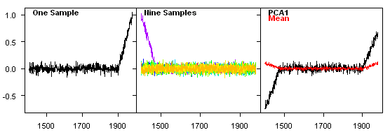
Figure 4. Ordinary PC method. Weights are 0.67 and -0.94 to two "dominant" series and under 0.02 for all others.
Figure 5 shows the same set-up using the Mannomatic. So this effect happens under ordinary PC methods as well as the Mannomatic. I’m sure that the effect is more intense or more frequent in the Mannomatic in some sense which could be defined but I’ve not had occasion to precisely de-limit it.
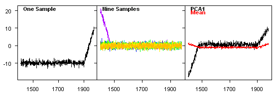
Figure 5. As with Figure 4, Mannomatic version.
For Figure 6, I’ve modified the setup of Figure 1 so that 9 series contain an actual "signal" using an ARMA(1,1) method (ar =0.9; ma=-0.6) to look like ARMA features of many actual temperature series. Then I’ve added in white noise as above. I picked a standard deviation for the signal that I thought would illustrate the point, but I didn’t fiddle with it to get this result. Figure 6 shows the PC1 using a conventional calculation. In this case, the outlier pulls the average up a little bit at the close, while the PC1 picks up the signal a little better than the average.

Figure 6. As with Figure 1, but 9 series also have a "signal".
Finally, Figure 7 shows the Mannomatic. In this case, the Mannomatic PC1 completely misses the signal and picks up the HS instead.

Figure 7. As Figure 6, but with Mannomatic.
The examples here don’t illustrate the extraction of the HS from red noise series where none of the series have a HS shape (discussed in GRL) . This effect was again denied by Mann at New Scientist, but exists nonetheless. Obviously in the above examples, there is a HS example in each of these series. Von Storch and Zorita asserted that the "Artificial Hockey Stick " effect was characteristic only of red noise environments. I think that our Reply to VZ gave a good response to this, by pointing to the effect of "bad apples" – which "steered" the algorithm even more.
Now one reaction to the signal examples might be to say: well, using the Mannomatic, we missed the signal in the PC1, but we got it in the PC2 (which is Presiendorfer significant.) That would be true in this toy example and in examples of practical interest. However, the problem with the Mannomatic is not that, given enough PCs, that it doesn’t recover the "signal", but that it will recover things that aren’t signals and they look Presiendorfer-significant. We’ve shown examples with tech stocks – sure, the Mannomatic can pick out tech stocks, but that doesn’t make them temperature proxies.
The Mannomatic has some ability to recover an actual signal, but the search for HS-series is strongly distorting that search. That’s why it finds the bristlecones, which actually do have a HS shape. Remember how we found the bristlecones. Once we noticed the data mining of the Mannian PC method, we asked: what does this do in the North American network? One of the outcomes of MM03 was that this network was isolated as what made MBH stand or fall – we didn’t know that in MM03 and didn’t know why the results were so different. When we applied this to the North American network, all the bristlecones bubbled out. We only found this by matching id-codes one by one to ITRDB identifications (since Mann had not disclosed this effect).
That’s how bristlecones came into the picture. Since the MBH version of the HS depends on bristlecones, that’s why we spend so much time on the question: are the bristlecones valid proxies? I don’t think that they are. But it shouldn’t matter. In synthetic examples where you have an actual signal, you can remove one class of proxies and still get a "robust" result. MBH should not be affected by the presence/absence of bristlecones. The inability to obtain a valid reconstruction without bristlecones (which Wahl and Ammann acknowledge, although they express it in different terms) shows that either all the other proxies are no good or the MBH method is no good or both. Ross’s rhetorical question to MBH is: why even bother with the other proxies?
The effect is particular damning because they claimed that their HS wasn’t affected by the presence/absence of dendroclimatic indicators altogether. If it’s not robust to bristlecones, this claim is obviously untrue. Has anyone ever seen an answer to this problem from the Hockey Team? This was one of the Barton questions. Mann didn’t answer it. We raised it with the NAS panel and we’ll see if they deal with this thorny question.


81 Comments
Thanks for the informative tutorial, but I think you left out another important feature of the “Mannomatic”. It can generate a hockeystick from the mean as well! (when you re-scale the variance to one).
It slices, it dices…
TCO has asked a lot of questions of Ross regarding PCA in another thread. One of his questions is, if I have it right, why should Mann not retain bcps in the PC4 when the data are properly centered even though it is not in the PC1?
Besides what Ross has answered, I think that there is one other important reason why bcps mean little or nothing in the PC4. The purpose of combining variables into PCs is to create a set of new variables that are linearly independent. That is, the PC1 is uncorrelated with the PC2 and so forth. See for example the explication of PCA in this link:
http://www.dcs.gla.ac.uk/~mc/1stYearReport/2.6_PCA.htm
As a result of the way PCs are constructed, if bcps are not present in the PC1, and if we know that absent a few series like the bcps there is no correlation between these series and temperatures in the twentieth century, then the fact that the PC4 is uncorrelated with the PC1, PC2 and PC3 tells us that bcps explain next to nothing in the analysis. Otherwise, they would be in the PC1, because the PC1 contains the series that have the most correlation with the variable to be explained.
Steve M: You may want to change the label in the second panel of figure 2 from “Nine Samples” to “99 Samples.”
This helps a lot to us non-statisticians, Steve. Thanks.
Yes, Steve, it helps a great deal.
I think “9 samples” means 9 tree-rings, not time samples.
Mark
In some cases, my questions may be studentish, or may require studentish answers to satisfy my questions. But in general my drift is not studentish, it is critical. And in some cases, on the other thread, the “studentish” comments about PCA did not even address my questions. (And it’s fine to say, “I don’t know” or “I won’t bother looking at it”. But one shouldn’t confound the debate (in that thread…) with non-responsive, long answers. I mean many of my questions were very simple: what percent does the “hockey stick index” change as a result of this error. I don’t need Mannian “it doesn’t matter” (analagous to the r2/RE kerfuffle) in response, without even the courtesy of an “I don’t know”.
And realistically, I take a cited error less seriously if we don’t quantify it’s impact. Or if I do have to pull teeth to get a quantification and then find (grudgingly) that the answer is that it has small effect. I also think an error that materially affected the hockey stick (in MBH98) is more interesting than an error which did not (but might in some other application of the method to another problem). I think the main direction of MM’s criticism and the importance of their articles has been related to the specifics of the hockey stick. Not to methodological issues for other problems.
Yes, they should have had to. But obviously they got away without having to. Now if you wade into an examination and criticism of the method, it’s incumbent on you to quantify impacts. You would never have gotten published by writing a paper that said “Mann should have had to better justify his method”. That was water over the dam. Your paper was a paper evaluating his method (critically).
Glad to see you making divisions and thinking like this. It’s distracting when one tries to drill down on a particular issue and gets non-responsive answers that scream about other issues than the one in debate. There may be a million warts on MBH. But when I examine a particular one, I want to figure out if it is a wart or a pimple. I don’t want someone showing me a wart on some other part of the body.
You should be publishing new results in new publications. New analysis in replies should only be done in a very selective manner. The replies suck anyhow. They’re not good papers (not just for the 35 yo professor props issue, Steve–but for explaining ideas the way you could in a more original paper.)
1. Is it nescessary TO AVOID it? your justification seems strained. If it doesn’t matter, then why do I need to supply a reason for “not avoiding it”. Instead, you can supply a reason FOR AVOIDING it.
2. The bigger concern that I have with white or particularly with red, is that there will be some different interaction of noisy series, of autocorrelation with the basic concept of PCA versus mean. (Not expressing this well, I know…)
Steve,
Thanks for digging into this and starting to do math to examine the issues. I have a long post following. Please take the parsing as a compliment (since I’m engaging in the issue details). Sorry about the profanity and such. I was drinking heavily while reading.
****
HS index (by eye, would like the real values, but “need an excel spreadsheet”):
FIG1.
sample 1: 1.0
sample 2-10: 0.0
PCA1: 0.95
mean: 0.10
FIG2:
sample 1: 1.0
sample 2-1000: 0.0
PCA1: 0.95
mean: 0.01
FIG 3:
sample 1: 20.0
sample 2-10: 0.0
PCA1: 19
mean: 2.0
BTW, why do you change the numbering here to a larger range and why do you have the sample 1 go from negative to positive?
Also, be careful about labeling/thought process here. Is this the “mannomatic” result (i,e, the hockey stick?) or is it the mannomatic’s PCA1. Give the mannomatic it’s due. It is the whole shebang! And I come back to my implicit “calling of Ross on the carpet”. Let’s be clear about the hockey stick itself (and how it was influenced) versus the PCA1. And (simply) what is “mannomatic” doing different from regular PCA in your example here.
FIG4:
sample1: 1.0
sample2: -1.0?
sample: 3-10: 0.0
PCA1: 0.0 or 2.0? or?
mean: 0.0
(I’m forgetting the definiton of hockeystick index.)
EVERYTHING CAN BE ANALYTICALLY SEPERATED. Even if there is an interaction of A and B, we can still consider the impact of “A” versus the impact of “A and B”. Don’t make me get all Rickover on your ass.
The graph in the paper points down? The simple average points down? What do you mean? What’s the exact definition of “the MBH99 HS”? Link to your old remarks?
Well…”get hot” as we used to say in the Nav. The picture actually shows very similar or even less mannomatic impact (the tail (variablility in the 1500s) is more, and the “blade” (variability in the 1900s) is less than in “regular PCA”. And I reiterate my concern about “the complete mannomatic” versus PCA1. How do we know that the other PCAs (orthogonal and all that) won’t give the Paul Harvey rest of the story. It still ends up being pretty screwy. But maybe not as bad as you make it look by only “Rossing it” in looking at PCA1 versus the actual Hockey Stick end result.
The OTHER FASCINATING THING is that your criticism seems much more relevant if it is a criticism of PC analysis per se! And not an analysis of the mistakes of Mann in using PCA. Maybe off-centeredness is not the big deal and the main battle should be enjoined on PC or no PC. (and you cloud the issue if you bitch about a “how to use PC properly” issue when the major damage is from using it even if you use it “right”) HA! Go f***ing NAVY! Oo-rah!
Fig 5 HS index numbers:
blablabla (Steve fill in)
Clarification question: when you have 9 white noise or 9 ARMA series. Are they DIFFERENT series or 9 exact copies?
Clarification question: are the ARMA coefficients only giving degree of autocorrelation or is there real signal in there, they way I would think of in a sloping line or a hockey stick? I mean is it just “nature of noise” or do the numbers give info the way a polynomial coefficient would?
Fig6/7: Steve fill in numbers.
AHA! Figure 6 versus 7 in comparison to 1 versus 3 shows a VERY interesting result! Why does the Mannomatic PCA1 differs so much from regular PC1 when red noise is used and so little when white is used!? I feel totally validated in probing this. Because it shows that there is more than simple offcetneredness causing an effect, it has to happen in combination with a particular type of noise. AHA! m***f***ing AHA! (but we still need to make sure we worry about the HS overall, not just the PC1.)
I don’t know about that. It sure looks like red noise gives different effects. And the “few bad apples” is a different issue! Non-responsive. HA!
Damn good and relevant point and one that we need to watch Ross like a hawk on, to make sure that he doesn’t confound the issues.
Well…yeah…maybe…but that’s still a different issue in any case. The wart on the face does not make the pimple on the neck a wart just because the wart on the face really is a wart on the face. Oh…and I wonder if this is an issue of the MANNOMATIC or is it an issue of PCA in general. Let’s watch this!
I SAY AGAIN, how much does the “mining” overpromote bristlecones IN THE FINAL HS, versus a SIMPLE AVERAGE or versus “non-mining PCA”. (lack of geographic weighting is a DIFFERENT ISSUE…and I damn well won’t let you confound warts.)
Now you are bobbing and weaving, buddy. A better logical analysis would be: the issue of their validity as proxies is a seperate question, but in any case, we can say that they are overweighted by X% or what have you. That’s the important concept. The issue of robustness to exclusion of a subsample is a seperate tool for criticizing the subject (and at some point, anyone can exclude examples and change the result for any stats analysis…so be careful here…it may be valid to use this as a robustness test, but is that ALL you’re banking on? Or do the methods faults matter in and of themselves?
#11. I spend lots of time worrying about autocorrelation and am not worried about this. Singular matrices can produce funny results and are best avoided. I noted this to keep track of the issue in case I wanted to re-visit it. Also in the Mannomatic, standard deviations are used and I didn’t want any division by 0. I was trying to finish something and go play squash, so I didn’t want to waste time in case singularities screwed up the calculation, when they were easy to avoid. Looking at the graphs, I’m certain that adding a little white noise doesn’t affect any of the points. But even if it did, the situation with the noise is a better representation of practical situations so it’s a better base case anyway.
How would a figure 4 (or 5) type example work if the two different series were blade up and down examples vice backward and forward blades?
But we would want to know “even if it did” that “it had”, since it changes the explanation from one purely based on offcenteredness interacts with signals to how “offcenteredness” interacts with noisy signals.
Most of your figures for conventional PC analysis are misleading. You are comparing PCA1 to mean as if PCA1 has an intrinsically meaningful scale, when it does not. If you rescaled your comparison plots so that PCA1 and the mean had the same variance, then the results would be nearly indistinguishable (aside from questions of orientation).
I do not believe such near equivalence holds for the Mann, offset-centered method.
#16. DF, the logic of using the same scale in the first couple of cases is that the PC1 is a linear combination of the series themselves, and, in the first couple of cases, for example, the loadings on series 1 are nearly 100%. Thus the PC1 is essentially an alter ego for series 1 and maintaining the same scale illustrates that.
The point of the other cases is also unaffected by re-scaling. For example, in the last two cases: in one case, the PC1 recovers the "signal" common to 9 of 10 series. In the other case, the Mannian PC1 recovers the hockey stick and misses the "signal". This is nothing to do with variance re-scaling.
This also applies to Figures 4 and 5. The PC1 flips over the early HS while the mean does not. The “topology” of the PC1 relative to the mean is different and has nothing to do with variance re-scaling.
Having said that, I’ll present similar results with variance re-scaling to show the effect in some simple cases. Variance re-scaling is something that’s crept into paleoclimate studies and is something that I’d planned to discuss at some point.
Steve, if you find objectionable what I find routine, then perhaps I don’t have a clue what you are doing.
The first step in conventional PCA analysis of scale-free data [and I presume tree ring networks are scale-free, since it is easier to scale to temperature at the end than to try and scale each tree at the beginning] is to subtract the mean from each series and then normalize each series to unit standard deviation. Then you’d compute the PCs (eigenvectors of the covariance matrix, etc. etc.) and rescale them to a physical record (e.g. insturmental temperature) to make the whole thing dimensional again.
This is why I find it objectional that you show the PCA1 and mean on such different scales, since in any scale-free context in is only the shape that matters.
However, on reflection, I realize that you never would have gotten the result you did if you had actually done what I expected. Since all 10 series are uncorrelated, if you had rescaled to unit variance, then PCA would have no reason to latch onto the hockey stick, since it would have been scaled to have no more variance then any other record. So I guess my question becomes, what is really done in a temperature reconstruction. It strikes me as implausible that each tree in a network would be individually calibrated to temperature. At the same time, I wouldn’t want to just let the tree with the largest variations dominate the reconstruction (hence the point of rescaling).
So, if they are doing what you are doing, and simply using PCA to effectively select the series with the largest variance then I would agree that this is problematic, but I can’t imagine why one would choose to approach it that way.
Oh, and I didn’t miss the other points, I just didn’t feel like commenting on them. Though to be fair, your tail flip example only occurs because the head series and tail series are so uncorrelated (or I suspect weakly negatively correlated). If the head series and tail series had any meaningful correlation at all it shouldn’t flip like that. If tree rings are any use at all in determining climate they ought to have enough correlation to prevent artifacts like that. (Whether or not they actually do is perhaps a topic for a different thread.)
#18. I was trying to illustrate some things here using toy models. I’m obviously aware of the points that you’re making. I’ll try to reconcile the points tomorrow. In a tree ring context, an issue that I did some experiments on about 6 months ago was to test breakdown points for the ability of various algorithms to recover actual signals in the presence of noise by blending in more and more noise. THe MBH method can pick up strong signals, but is easily confused by its off-centered methods which mine for hockey sticks. The MBH tree ring networks are an absolute pig’s breakfast so the HS mining takes over. I’ll post some more on this.
A few words about the Bristlecone Pine (BP) data – my 10 pence worth to the debate.
Certainly, if these data dominate a NH reconstruction through the use of PCA, this is probably not an ideal situation where presumably a NH reconstruction should be representative of the NH.
However, how valid are the BP data as a ‘local’ temperature proxy?
At the link below, I have uploaded some pictures comparing BP data with the North American (NA) mean series from our 2006 paper. We never included the BP data in our paper as we wanted to use as high latitude TR data as possible. However, the inclusion of the BP would have made little difference to the final NH reconstruction, although it would have depressed the MWP a little relative to the recent period.
http://freespace.virgin.net/rob.dendro/NAvsBP/NAvsBP.htm
———————-
Figure 1 – a comparison of our NA mean with a RCS chronology developed using BP RW data from three sites: Hermit Hill (N = 38; 1048-1983) and Windy Ridge (N = 29; 1050-1985) from Colorado and Sheep Mountain (N = 71; 0 — 1990) from California. The time-series have been normalized to the 1200-1750 period.
A couple of interesting points:
1. at least for the 1100-20th century period, there is a surprisingly strong common signal. From this comparison alone, one could conclude that, although the BP data represent a relatively small region (in a global sense), the data do seem to pick up the multi-decadal to centennial scale variability of the larger NA mean series. The deviation between the series prior to 1100 may simply represent the decreasing replication of NA sites – there are only two sites that go back prior to 1100 in the NA mean. As stated in our paper, I do not feel there is enough data prior to ~1400 anyway.
The BP RCS chronology correlates with ‘local’ July-September mean CRU gridded temperatures at 0.38 (Durbin-Watson = 1.70). This is admittedly not particularly strong (NB. no autocorrelation in the residuals though), but with the reasonable comparison with the NA mean, it does seem to suggest that temperature is likely the dominant controlling factor – especially at decadal to longer time-scales.
Now, I do not deny that all sorts of other factors may also influence growth and I am sure someone will say – ‘well how about all the none explained variance?.’ Well – Dendro-reconstructions generally explain anywhere from 30-60% of the variance of the climate parameter that one is trying to reconstruct. This is a modeled mean response over a particular [calibration] time-period and does not look at the more complex situation for each year. Using regression, it is easy to test if multiple climate parameters (i.e. temperature and precipitation) effect the growth of trees. It is generally the case, that if the tree site is carefully selected (i.e. high elevation/latitude treeline for a temperature signal), then precipitation will have a minimal effect on growth and over the period of calibration, the correlation with precipitation will be close to zero.
2. I purposely normalized the data to the 1200-1750 period so that any possible inflation of BP index values due to CO2 fertilization would be accentuated relative to the NA mean. Interestingly, the NA mean index values are higher than the BP data. Assuming that no CO2 fertilization effect biases the NA mean (there is no evidence for this at all), then I see no evidence of this effect in the BP data either.
———————-
Figure 2 – comparison of the NA RCS mean with the recently published annual temperature reconstruction for the Colorado region from Salzer and Kipfmueller (2005). They also used BP data – independent to the data I used. There model explains 46% of the variance (DW = 1.64), so is appears to be a much stronger temperature proxy than the one I showed in Figure 1. Again we see reasonable coherence between 1100-1900 and again the BP data do not show higher values in the 20th century than the NA RCS mean. Salzer and Kipfmueller did not use RCS for detrending so it is possible that they have lost some long term information.
———————-
Take home message – I do not think the BP data are as bad as Steve would have us believe.
OK – a little more – a pounds worth.
Rob
Rob: Looks like a decided downward trend in “temperature” in recent years. Does your paper conclude that we have an AGW problem?
Rob: I like the fact that you had an a priori reason for selecting tree series–high elevation. I’m not so sure that drought isn’t a factor there, however. The soils tend to be very shallow and sandy, without much water-holding ability.
#21 jae, I think that your question here is part of the problem in discussing these issues. Rob has provided some arguments about the Bristlecone Pine in how it should be considered as a proxy for temperature. Just as it is right to complain about extrapolations for AGW from a single study. It is equally unfair to ask a scientist to reject AGW based on a single study. There are no magic bullets for either position.
I purposely normalized the data to the 1200-1750 period so that any possible inflation of BP index values due to CO2 fertilization would be accentuated relative to the NA mean. Interestingly, the NA mean index values are higher than the BP data. Assuming that no CO2 fertilization effect biases the NA mean (there is no evidence for this at all), then I see no evidence of this effect in the BP data either.
Re: 23
You have it upon something that has been bothering me for some time. Many of the AGW supporters have called people on this blog “deniers”, but that’s really an unfair characterization. At this time the data on AGW, or even GW, do not support any conclusion. The uncertainties are just too great to claim that the theory is correct or not. So we are not denying that GW or AGW is occurring, per se, but we are still trying to wade though all the claims and counter-claims, and trying to apply sound scientific and engineering principles to find out what’s true and what’s not.
Now I’m sure that there are some true believers here on both sides of the issue, but most of us don’t fall into either of those camps.
I wish I could edit my own postings. I meant to say “have hit upon something” in the first sentence there.
Oh come on, you guys, I know you can’t infer anything from a single study. I just want to know if the author has concluded anything about temperatures from his work, or if it was solely devoted to a comparison of bristlecones with other trees. Does he believe he has a good temperature proxy?
re #20
Looking at your figure 1, the thing that strikes me is how badly the curves match outside your normalization period. And while the agreement does continue back from 1200 to 1100, we know there’s lots of autocorrelation in tree-rings so that doesn’t necessarily mean much. But while I admit I’m not much familiar with RCS except for what I’ve read here and I don’t know how your trees / sites were selected and thus don’t know if any unconscious cherry-picking is possible, it is worrisome. The period outside of the the time you had control over, and particuarly time moving forward is what decides whether you’re actually making predictions or just curve-fitting. And while I’m sure you’d never curve-fit on purpose, assumptions about reality that we carry with us make it difficult not to make decisions as to procedure that have unrealized consequences.
Given the awareness we have of BPs as having a 20th century growth spurt, a trend upward in the 1900s isn’t surprising, but as jae pointed out, the NA mean trends down the latter part of the 1900s while the BPs don’t seem to so which is correct if either?
re: 25. I agree that we “don’t know” yet. But to a true believer in AGW, this position makes you a contrarian. IMO, since I don’t believe there is really a scientific consensus that AGW is a fact, maybe the true believers are the real contrarians. It’s all relative regarding who is a contrarian.
Steve- You’ve done a great job with this website and your demonstrations of “insignificance”. You’ve also been a great proponent of R. What would be a great help to some of the “not-so-swift” (such as me), would be to put in some R code snippets (along with some reference to whatever plotting program you are using), so that we could replicate what you are saying and doing on our own machines. (This would probably help TCO as well!) If you find this interesting, please annotate the R code. Thanks for considering this!
An observation concerning principle components has been stewing in my mind for some long time, especially since Osborn and Briffa used a PC1 as one of their 14 proxies in their (2006) Science 311, 841-844 paper, “The Spatial Extent of 20th Century Warmth in the Context of the Past 1200 Years.”
The observation is that principle components have no physical meaning outside of a physical theory. One uses PC’s to reconstruct a desired physical signal that is hidden within a data-set consisting of convolved single-origin signals. The reconstruction of any given particular signal from the total signal, using PC’s, is always the weighted linear sum of all the PC’s. The weights are calculated, for example, by means of an iterative fit to data in terms of all the PC’s, carried out within an explicit physical model of the system derived from theory and experiment; a model that also quantitatively specifies the number of physical components comprising the total signal.
The PC’s themselves don’t mean anything physical. They are only numerically orthogonal constructs of the data (call them projections of the data onto a set of orthogonal axes). Mann’s PC1 was never given any physical meaning by analysis within any theory of the environmental response of tree rings, or ice cores, or whatever. It has no physical meaning. For all anyone actually knows, PC1 could be pure low-frequency noise.
That means Briffa’s and Osborn’s use of PC1 as a legitimate proxy to add to the other proxies was entirely wrong. It means that PC1 in MBH98,99 also has no physical meaning, and certainly can not be said to represent temperature. PC1 is an entirely meaningless result, physically, no matter whether it merely represents bristlecone extract (it apparently does), or were a legitimate PC1 that reflected the major variance of properly combined proxies, because there is no temperature-proxy theory to give it, or PC2, PC3,…, any physical meaning.
Either O&B don’t know the meaning of principle components, (and neither do the reviewers or editors of Science), or I’ve got it all wrong, or O&B do know that PC1 is physically meaningless and proceeded to use it anyway.
And if I’m right, then all of the IPCC chiefs, plus all the scientists who touted MBH98,99 as the smoking gun of AGW, have parlayed a physically meaningless result into something scientifically specious.
I don’t understand how that could have happened — presuming my understanding of principle components is correct. Presuming that, how could so many scientists have let that false attribution go by without protest?
So, Steve M. — do I have PC’s right?
Pat, I’m not sure if you do or don’t have PCs right, but let me make a stab at what the Hockey Team might say. Their assumption is that tree ring widths or maximum densities are linearly related to temperature (T). I.e. they say W(x)/T(x) = C [where x = a year and C a constant]. Of course they recognize that there’s lots of other factors and noise besides, but they assume these will cancel out over time. So by calculating C for a lot of years corresponding to the training period, they assume they can then use W(x) for earlier dates to estimate T(x). This, it seems to me is a physical theory, though it has problems which have been discussed here in various threads. So I don’t think your complaint will work without showing either that the relation to temperature isn’t linear or that the other factors don’t cancel, either of which are good possibilities.
Dave, the Hocky Team supposition, as described, is a hypothesis at best. More accurately, it would be a hunch that needs testing.
To really use principal components, they’d need an analytical theory of tree ring widths. A simple example might be RW = f(T)+f(M)+f(ranV), where F(T), etc., is ‘function of temperature,’ ‘function of moisture,’ and ‘function of random variation (such as episodic fertilization).’
These functions could be complex and non-linear. A time-wise proxy series contains elements of all relevant variables. A principal components analysis would yield PC1, PC2, PC3,…,PCn, where every PC would also contain all of those variables in unknown ratio. The PC’s are just intensity-ordered numerically orthogonal traces of the graphical variance of the data series. They have no particular physical meaning.
To do the analysis, one would reconstruct the analytical theory in terms of the PC’s, with each function T, M, ranV, expressed in terms of a linear combination of PC’s.
I.e., RW=f(T,sum1[PC’s])+f(M,sum2[PC’s])+f(ranV,sum3[PC’s]), where sum1, sum2, and sum3 are weighted sums of the PC’s. Each sum is unique in that the PC’s have different weightings.
The coefficients of the summed PC’s would be weighted by an iterative fit to the proxy series. If the PC analysis yielded 3 PCs, for example, then the outcome of the iterative process in terms of the theory would yield Temperature trace = c1xPC1+c2xPC2+c3xPC3, where c1-c3 are the iteratively best fit coefficients. Likewise, Moisture trace = c4xPC1+c5xPC2+c6xPC3, where again the c4-c6 are best fit coefficients.
The physical meaning comes from the weighted sum of all the PC’s within the analytical context of a theory that allows determination of the weighting coefficients as constrained by the physical form of the equations for temperature response, moisture response, and so forth.
All by themselves the PC’s mean nothing, physically. The MBH PC1 is physically meaningless. It doesn’t matter at all whether RW is linear in T. For all anyone knows, PC1 could reflect mostly a moisture signal; or something else. Absent an equation-expressable theory of ring widths that can be parameterized in terms of weighted PC’s, PC analysis of a ring width series is scientifically sterile.
The only way a PC could mean something by itself would be if a signal is known from theory to consist only of a single variable plus noise. One could use PCA to then extract the signal from the noise. What Mann & co. are claiming in giving physical meaning to PC1, essentially, is that his proxy series includes only a temperature signal plus noise. There is no physical theory to validate that claim. PC1 is no more than a-scientific propaganda.
Which is why I criticize Ross when he talks about PC1 in isolation.
Right on! I am still waiting for someone to point me to a study of any kind that shows that trees are sufficiently sensitive to temperature (including a linear relationship) to justify all these “temperature reconstructions” using tree ring data. The whole crazy field of study depends on this basic relationship, and it doesn’t appear that it has been established!
Dano agreed to hook us up with some dendroclimatology experts, and some of urged him on; but, alas, nothing but dead silence. It appears that his bluff has been called.
Even if there were a relationship, I believe it is overshadowed, overall, by all the other variables critical to tree growth. Especially moisture, competition, and nutrients. I guarantee you, there is no relationship that consists of only temperature and random noise.
How about PC1 being the generalised anthropogenic fertiliser signal?
I see some remarkable resemblance to global population.
36. Good point. Has anyone calculated the total CO2 output from the 9 billion humans + their pets?
I would think humans don’t actually “output” CO2 as we are only exhaling what we’ve inhaled in the first place.
Mark
I have joined the “professionals” listserv for dendrochronology. Most of the posts are about things like work details. There is little discussion, but it is allowed provided you clearly lable it as such. I want to read some of the old postings, before I start some discussion.
38. No, we constantly inhale O2 and exhale CO2. I looked it up; we each exhale about 1 kg/day. But this CO2 is viewed as neutral, because we are really getting the carbon from plants, either directly or indirectly (by eating meat, fish, etc.). And the CO2 is then again used by plants. Same argument advanced for the neutrality of burning biomass. Sorry for the digression.
My girl friend is more concerned with my methane production, which is in fact, a more potent
gasgreen house gas.Re: #41
Apparently a third of all methane released into the atmosphere by termites. This leaves only 2/3rd to be a problem for your girlfriend.
Housekeeping transfer: 2006-6-28 @ 5:06:14 pm re #16/2. You still don’t get this best approximation property. I was able to locate the following short proof which I think you should read until you understand it: Arne DàÆà⻲: On the Optimality of the Discrete Karhunen–LoàÆà⧶e Expansion, SIAM Journal on Control and Optimization, 36(6), pp. 1937-1939, November 1998.
Hey SteveMC, check out Tamino, he’s got a post on this
Tammy town is a fun place to explore rhetorical probing missions.
When Tammy said he was doing PCA I figured he would get to the decentered issue.
I even praised him for educational efforts.
Now, we shall see how he extricates himself. Should be good theater. Popcorn is on me.
#44-45. Noted. Some of the contortions that people make on behalf of the Stick are quite amazing. I’ll post on this in due course.
Nice spot, mosh.
Just reading RomanM’s excellent response:
Which is, of course, the point, but just look at Tamino’s response:
So… if MBH98 didn’t pass verification, it could be a hockey stick plucked out of thin air? What were the verification statistics again, Tamino?
Perhaps this chap is smarter than he sounds.
Ah come on. What was wrong with that post?
#47 (MarkW): It’s complete rubbish. Ask your stats professor if you don’t believe me. Too bad, Tamino had three rather nice posts about PCA.
The strangest aspect of the series on PCA by Tamino, who I assume is a scientist, is that he was fine as long as he was talking about the mathematics of PCA. When he gets to the more scientific aspects (application, inference, interpretation) in part 4, he completely goes to pieces.
Jean S. is quite right.
Maybe he should change his hide-behind name from Hansen’s Bulldog to Mann’s Best Friend.
Oops, sorry, stepped on your toes, JS, but at least now he’ll have to post your comment since he’s noted that it is in moderation.
============================================
It is certainly worth going to read Tamino’s responses to Jean S.
=====================================
JeanS,
I was referencing the post that Steve deleted.
Ha, I thought so, Mark W, but am still amused. Happy Halloween.
=======================
They sure get their panties bunched up in knots over there.
I still want to know why my e-mail from the Directorate to start reading Tamino again wasn’t delivered.
re 57. I want it noted for the record that when tammy embraced the moniker “Hansen’s Bulldog”
I refrained from making the utterly obvious joke which would have used a different “B” word
clarifying the gender of said bulldog.
For the record.
MarkW — 57,
MarkW wins this thread. If I’d been drinking coffee it would have shot out my nose!
steven mosher,
Tamino should be a boy. According to Wikipedia, in act II:
“Tamino and Papageno are led into the temple. Tamino is cautioned that this is his last chance to turn back, but he states that he will undergo every trial to win his Pamina. Papageno is asked if he will also concede to every trial, but he says that he doesn’t really want wisdom or to struggle to get it. ”
Here is Lucia Popp, playing the part of Pamina, who is heart broken Tamino won’t speak to her. Tamino is the guy lurking in the background holding the flute. For an operatic hero, he is rather hapless.
But… I do have a substantive question for Jean S — does the “centering” problem have anything to do ill-conditioning issues? I know ill-conditioning is rife in statistical tests, and often people who only know theories end up falling into traps when they actually start to stuff in numbers.
Or is the centering problem something else.
#54 (MarkW) Sorry about that, I thought you were referring to SteveMC’s comment.
#52: kim, no problem. Actually I think he would not have published my comment unless you had made your comment. In fact, this “open minded” Mann’s bulldog, who ends his post by saying “In the meantime, I have one request: before you raise other issues about the hockey stick, address this one.” did not allow me to address his post another time. For the record, this comment did not go through:
Jean S, it is my understanding that Jolliffe was referee #1 in the first Nature review and referee #2 in the second Nature review – see here (Permission was given to me to post this and other reviews.) The reviwewer said (and some of his remarks echo yours):
Our Nature resubmission is here.
Jean S,
Here is my comment to Tamino (also awaiting moderation):
If Tamino were to get something published, I am certain you or UC would be happy to rebut his errors.
http://www.funnyordie.com/videos/62f250455c
I love this guy… your musical interlude.
According to Tamino, the verification period was just prior to the calibration period. Does anyone know what was the verification statistics for MBH? I see hints here that it was not good.
Jean S , EW
Thanks for reporting those censored comments. Sometimes the words you are not allowed to say at RC or related blogs are surprising.
Re 60,JeanS
I had wondered why you hadn’t responded to Tamino and now I know that you did but were censored. I have to ask, tho, why you used strong language, like BS, in your original post and response. BS it may be, but to get your message heard wouldn’t it be better to write respectfully?
I have heard a saying attributed to Plato:
When you use insults and loaded words, you show that you are arguing with a fool and encourge your interlocutor to do the same.
This is what Tamino answered to my question why he didn’t released Jean S’ answer:
And my follow up post does not seem to have made it on to Open Mind. Not sure why. But rather than waste that typing let me post it here, typos and all.
#
mikep // March 9, 2008 at 12:02 pm
Just a couple of points of clarification. I’m sorry to go over old ground. But what amazes me about all this is that when obvious errors are found people don’t accept them and go on to better work but refuse to admit tehy were wrong. This attitude has made me significantly more sceptical about how well founded significant AGW is.
On adjusting for carbon fertilisation I quote from M&M’s 2005 Energy and Environment paper.
“Mann et al. [1999] purported to adjust the NOAMER PC1 for CO2 fertilization, by
coercing the shape of the NOAMER PC1 to the Jacoby northern treeline
reconstruction in the 1750–1980 period, arguing that the northern treeline series would
not be affected by CO2 levels. Once one gets into such ad hoc adjustments, many new
questions need to be answered about the validity of the adjustment procedure. In the
actual Mann et al. [1999] adjustment, the main adjustment for “CO2 fertilization”
takes place in the 19th century rather than the 20th century, with Mann et al. [1999]
being forced into the counterintuitive position that the effect of CO2 fertilization was
somehow stronger in the 19th century but became attenuated in the 20th century, the
exact opposite of the hypothesis of LaMarche et al. [1984] and later Graybill and Idso
[1993]. If the differences between the northern treeline series and the bristlecone pines
arise from some other factor (a couple of possibilities are discussed below), then the
Mann et al. [1999] “adjustment” would have made the proxy record even more
distorted. In MBH98, no such adjustment was made in the AD1400 period in any
event.”
There is evidence – see Mr Pete’s contribution – that the anamolous 20th century growth in strip-bark bristlecones is not due to carbon fertislation. I note that in any case such an adjustment does not in any way deal with the divergence (not diversion) problem. This is that the bristlecones in question have not shown exceptional growth in the late 20th century when the global surface temperature has been increasing at a faster rate. If they can’t pick up recent temperature rises what reason do we have for assuming that they have picked up all similar rises in temperature in the past?
This divergence provides a much more dmeanding test that separting known data into a claubration and verification period. However we need also to note that MBH did fail in teh verification period chosen. Again from Energy and Environment 2005:
“Most dendroclimatic reconstructions
provide a suite of verification statistics, including RE, R2, CE, sign test and product
mean test [e.g. Cook et al, 1994]. In MBH98, only the RE statistic is reported for steps
prior to the AD1820 step, including the controversial AD1400 step. Mann et al. have
not provided their own results for the other verification statistics or supporting
calculations from which these statistics could be calculated, and have refused requests
for this information. McIntyre and McKitrick, 2005, using Monte Carlo simulations,
shows that the MBH98 benchmark for 99% significance for the RE statistic is
substantially under-stated (0.0 in MBH98 versus a Monte Carlo estimate of 0.59) and
that the R2 and other verification statistics, which were not reported in MBH98, are
statistically insignificant in the AD1400 step.”
There has been some subsequent controversy about the exact level of the RE statistic which is significant (my reading is taht it still fails), but the RE test is not an especially demanding test and there is no doubt that the reconstruction fails on the other statistics.
It looks to me as though data mining for hockey stick shaped proxies has resulted in a classic spurious regression with good in-sample fit and very poor out of sample performance.
Your comment is awaiting moderation.
Tamino:
I don’t buy that. I think it was the substance of the second post (the one that got censored). Of course it gets personal, careers of those guys seem to be dependent on MBH9x. What a terrible situation for them.
Tamino:
It’s just pitiful; neither the tree rings, nor the thermometers are following the hockey stick, anymore. Only CO2 keeps rising, and even the unwashed can sense a problem there.
========================================================
re 69. Comments designed to annoy tamino: 2+2=4. and other assorted truths
#72
2+2=4 is only true for sufficiently large values of 2. But let’s turn to the models and see what they have to say.
In looking at the backgrounds of the combatants, I modestly propose
Sherrington’s Postulate 2008:
“The value of a scientist is enhanced by the experience of hurt from personal falure; it is more greatly enhanced by the enjoyment of acknowledged personal success.”
Rider. When the scientist has no objective test for success or failure, do not use this Postulate.
Jonathan says: “2+2=4 is only true for sufficiently large values of 2. But let’s turn to the models and see what they have to say.”
ha ha ha ha!!! priceless
Re: #66
After reading the exchange, I strained my brain to come up with better terminology for Tamino’s responses and I kept coming up with BS and more BS. Contrast Jean S’s measured response in terms of how a statistician would handle the process using accepted practices and how Tamino deals with it with partial averages and Rule N. I do not think one needs to be a practicing statistician to see that those attempting to rescue the MBH methodology tend to use a lot of BS — creative and inventive, but BS just the same.
Somebody give tammy homework for the week
http://web.grinnell.edu/individuals/kuipers/stat2labs/Handouts/GW%20Paper%20USCOTS.doc
Would that be in cartesian or polar coordinates?
Nice follow up Post on tammy RomanM. I have to thank you here, since I’m BOOM. Banned On Open Mind.
Thanks mosh. On the weekend I did some readin’ and thinkin’ and thought that the best approach was to do the math and look at the effects from that angle. I was pleasantly surprised by the very polite reception since on one occasion earlier he had lumped me in with bore hole climatology ( I couldn’t tell my ### from a hole in the ground). I give him credit that he has never kept any of my posts there from appearing as is.
re:#79, 80, 81
The S/N over there is so tiny it’s difficult to determine that tamino has responded to fine technical issues with a fine technical response. Generally so it seems to me, he dodges the toughies and always plays to his peanut gallery. The tech/nontech content there is also tiny, Imho.