MBH and Partial Least Squares

Right now, I’m working on two main projects where I intend to produce papers for journals: one is on the non-robustness of the “other” HS studies; the other is on MBH98 multivariate methods. The latter topic is somewhat “in the news” with the two Bürger articles and with the exchange at Science between VZ and the Hockey Team goon line of Wahl, Ritson and Ammann. (“Goon” is a technical term in discussion of hockey teams: Hockey Teams all have enforcers sent out to fight with and intimidate opposing players.)

From work in progress on the second project, here are some comments on the linear algebra in Bürger et al. Contrary to B-C claims that MBH98 methods cannot be identified in known multivariate literature, I show that – even though this is seemingly unknown to the original authors and later commentators – MBH98 regression methods can be placed within the corpus of known multivariate methods as one-factor Partial Least Squares (this is probably worth publishing by itself although it opens the door to other results) . (Update – I’ve edited this to reflect comments from Gerd Bürger, which have reconciled some points.)

While there is much to like in Bürger and Cubasch 2005 and Bürger et al 2006, they were unable to place MBH98 within a multivariate framework, stating:

MBH98 utilize a completely different scheme which one might call inverse regression. (To our knowledge, no other application makes use of this scheme.)

They summarize the algebra of MBH as follows:

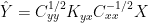
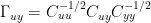
There, one first regresses x (proxies) on y (temperature) and then inverts the result, which yields, according to eq. (5), the linear model
$\hat{y} = C_{yy}^{1/2} \Gamma_{xy}^+ C_{xx}^{-1/2} x$

where the “+” indicates the Moore–Penrose (pseudo) inverse, with $C_{xx}$ , $C_{yx}$ , etc. denoting the cross-covariance between x and x, and y and x, respectively and using the matrix
$\Gamma_{xy} = C_{yy}^{1/2} C_{yx} C_{xx}^{-1/2}$

Here’s what I agree with and disagree with in this formulation:

1) I agree that the reconstructed PCs are linear combination of the proxies (as is the NH temperature index), a point that we made as early as MM03, although a contrary view is expressed in Zorita et al 2003 and von Storch et al 2004;
2) I think that this is a cumbersome and infelictous algebraic expression, although I’ve now reconciled it to my own notation. It’s obviously not expressed this way in MBH98 – this is how B-C characterize MBH98, not what MBH said they did. I think that there are some important cancellations.
3) Because Bürger et al have not carried out all possible cancellations (and in particular have not focused on the one-dimensional case which governs the MWP), they’ve been unable to place MBH98 within the universe of multivariate methods. I’ve referred in passing to the placement that I’ve derived and will show a few more details today.
4) I’m still checking on how Bürger dealt with re-scaling.

It would be amusing if B-C was one more instance of commentators not quite implementing what MBH98 actually did. In terms of robustness issues, I don’t think that this would affect their non-robustness conclusions, but it might affect specific results. The continuing inability of commentators to place MBH98 methods within the vast corpus of multivariate methods is surely intriguing. As a follow-on, I think that a couple of later studies have ended up, using methodology that is formally equivalent or near-equivalent to MBH98 without being aware of it and even describing the methods as novel.

Some History

The viewpoint that the reconstructions is linear in the proxies was one that we expressed as early as MM03 as follows:

It should be noted that each of the above steps in the MBH98 northern hemisphere temperature index construction is a linear operation on the proxies. Accordingly, given the roster of proxies and TPCs in each period, the result of these linear operations is a set of proxy weighting factors, which generates the NH average temperature construction.

Similar comments were made in MM05b (E&E). An opposing view was expressed in Zorita et al 2003 as follows:

“The optimized temperature fields target the whole available proxy network at a given time, so that the inclusion of a few instrumental data sets in the network should have little influence on the estimated fields, unless the instrumental records are explicitly overweighted. The advantage is that the method is robust against very noisy local records. This contrasts with direct regression methods, where the estimated temperature fields are the predictands of a regression equation. In this case a few instrumental records, highly correlated to the temperature fields, may overwhelm the influence of proxy records with lower correlations in the calibration period.”

Von Storch et al 2004 took the same position as Zorita et al 2003 that the effect of individual proxies could not be allocated:

“MBH98’s method yields an estimation of the value of the temperature PCs that is optimal for the set of climate indicators as a whole, so that the estimations of individual PCs cannot be traced back to a particular subset of indicators or to an individual climate indicator. This reconstruction method offers the advantage that possible errors in particular indicators are not critical, since the signal is extracted from all the indicators simultaneously.”

Obviously our viewpoint – that individual proxies i.e. bristlecones – had a dramatic and non-robust impact on MBH98 results was at odds with the viewpoint expressed by VZ. B-C agree that the MBH result is linear in the proxies. So I think that the earlier viewpoint of VZ has been definitively superceded (and it’s a view that Eduardo held passim rather than strongly). I don’t make this point as a gotcha, but because I think that it is extremely important to think in terms of estimators formed from linear combinations of proxies in order to think mathematically about the various issues in play.

MBH98 Linear Algebra

Earlier this year, I posted up linear algebra showing that the reconstructed PC1 was a linear combination of the proxies with weights proportional to the correlation coefficients to the target temperature PC1, followed by re-scaling; and that the NH temperature index was simply this series multiplied by a constant.

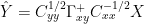
This first post showed this for the reconstructed temperature PC1. If u = U[,1] the temperature PC1 and ρ = cor (u,Y), the vector of columnwise correlation coefficients, then I derived the reconstructed temperature PC1 $\hat{u}$ as follows (before re-scaling):

(19) $\hat{u}= Y * \rho *\frac{ sd(u)} {(\rho^T *\rho )}$

with the result stated as follows:

That is, the reconstructed TPC1 in the AD1000 and AD1400 steps is simply a linear weighting of the proxies, with the weights proportional to their correlation to the TPC1.

In the next post here, discussing our source code, I showed that we re-scaled empirically and then extended the linear reconstruction to the NH temperature reconstruction, since all steps in this procedure are also linear. In the one-dimensional case, the RPC1 is just multiplied by a constant. However the re-scaling can be stated in linear algebra terms, yielding an expression for the re-scaled reconstruction as follows, if I’m not mistaken:

$\hat{u} = Y * \rho *\frac{ sd(u)} {(\rho^T C_{xx} \rho )^{1/2}}$

The simplifications and cancellations of this linear algebra are something that I’ve been working on for a while and am still working on. These results are not inconsistent with our code – they are equivalent to it. However, the cancellations involved here make it possible to condense about 20 lines of code into 1 or 2.

Contrary to what I’d posted earlier, I’ve worked through the linear algebra of the Bürger et al 2006 expression from first principles and can now reconcile their results to mine, although as noted above, I don’t believe that they have carried out all possible cancellations.

In terms of other studies, I have been unable to replicate Mann and Jones 2003. They appear to use proxies weighted by correlation coefficients. I corresponded with Phil Jones about this in an attempt to figure out what they did. Jones said that the weights did not “matter” and that similar results were obtained using unweighted average. This was false. I asked him what weights were used in Mann and Jones 2003; he said that he did not know, only Mann did, and terminated the correspondence. I think that Hegerl et al 2006 (J Clim) also use correlation-weighted proxies, but we’ll have to wait and see when it’s published.

One-Factor Partial Least Squares

Partial Least Squares is a known multivariate technique, commonly applied in chemometrics. Googling will turn up many references. Partial Least Squares is an iterative process and, after the first step, the iterations proceed through what have been identified mathematically to be Krylov subspaces, but these later subspaces are not relevant to the one-factor PLS process. The first step of Partial Least Squares also constructs an estimator by weighting series according to their correlation coefficients.

Bair et al 2004 has a concise formulation of this shown below, although the point can be seen in any multivariate text discussing

Comparing this formulation to the derivation in my post summarized above, in both cases the coefficients of the estimator are partial correlation coefficients. In the MBH98 case, the estimator is re-scaled to match the variance of the target – which is one of the PLS options. In the later MBH steps, more than one temperature PC is reconstructed, but each temperature PC is reconstructed through an individual PLS process. For the purposes of NH temperature, the estimate is totally dominated by the temperature PC1 and the lower order temperature PCs have little actual impact. In the 15th century step and the earlier MBH99 step, only one temperature PC is reconstructed anyway.

Multivariate Methods

Once one expresses MBH98 as a multivariate method within a known statistical corpus, it totally transforms the ability to analyze it both in terms of available tools and even how you approach it.

As noted above, PLS is commonly used in chemometrics, where it is viewed as an alternative to other multivariate methods, including principal components regression. Viewed from the perspective of linear algebra, all these multivariate methods can be construed as simply a method of assigning weights to the individual proxy series. Again, this is a simple statement, but it is well to keep firm memory of this when confronted with bewildering matrix algebra – at the end of the day, after all the Wizard of Oz manipulations, you simply end up with a series of weights, and there is no guarantee that all this work will do any better than a simple average. Indeed, in my opinion, the FIRST question that should be asked is: why aren’t we just doing an average?

The corpus of available methods is bewildering: multiple linear regression is one obvious multivariate method – in this case, the resulting weights are called “regression coefficients”. You could also do a principal components analysis and, if you truncate to one PC, the resulting weights are called the “first eigenvector” (which are then scaled by the first eigenvalue). Other named methods include ridge regression, partial least squares, canonical correspondence analysis, canonical ridge regression. Principal components regression is regression on the principal components. There are connections between most of these methods and there is much interesting literature on the connections between these methods (e.g. Stone and Brooks 1990; papers at Magnus Borga website; etc.)

More generally, surely all these multivariate methods are, from a linear algebra point of view, alternative mappings onto a dual space (the coefficient space). Each multivariate method is a different mapping onto the dual space. B-C do not construe their “flavors” in a multivariate method context. They generalize the non-robustness that we had observed phenomenonologically, but their consideration is also phenomenonological and doesn’t really rise to an explanation of what’s going on. (I’ve got an idea of what would be involved in a proper explanation, but doing so is a different issue.)

In this respect, it’s helpful to construe a simple unweighted average as also being a method of assigning coefficients in the dual space. When you read a good article like Stone and Brooks 1990, linking OLS, PLS and ridge regression through a “continuum”, it makes one wonder how one can go from OLS coefficients to coefficients for a simple average through a “continuum”. I’ve developed some thoughts along this line, which seem too obvious to be original and not wrong, but I’ve not located them anywhere.

If you do a simple average of the series after “standardizing” – this could lead to further variations involving robust measures of location and scale: perhaps using a trimmed mean as a measure of location and mean average deviation as measure of scale as alternatives to the OLS mean and standard deviation, which stand in poor repute among applied statisticians and standardization methods (see Tukey, Hampel etc.)

In the MBH case, it’s not just partial least squares. The tree ring networks have been pre-processed in blocks through principal components analysis; the gridcell temperature series have been pre-processed through principal components analysis on a monthly basis (and then averaged moving them slightly and annoyingly off orthogonality – but they are approximately orthogonal.) Some series are included in networks, others aren’t. However, I think that these are subsidiary issues and there is much advantage in separately considering the MBH98 regression module from the viewpoint of the known method of one-factor partial least squares.

Tomorrow I’ll show how a number of these methods apply to a VZ pseudoproxy network. The VZ pseudoproxy network is a massive oversimplification – it assumes that pseudoproxies add the SAME proportion of white noise to gridcell temperature. But because it’s so simple, you can test some things out before you move to more complicated red and low-frequency noise. My main beef is that results from this proxy Happy-world have been extended to situations where they do not apply.

References:
von Storch, H., E. Zorita, J. M. Jones, Y. Dmitriev and S. F. B. Tett, 2004. Reconstructing past climate from noisy data. Science 306, 679-682.
Zorita,E., F. Gonzàlez-Rouco and S. Legutke, 2003. Testing the Mann et al. (1998) Approach to Paleoclimate Reconstructions in the Context of a 1000-Yr Control Simulation with the ECHO-G Coupled Climate Model . Journal of Climate 16, 1378-1390.
Eric Bair, Trevor Hastie, Debashis Paul, and Robert Tibshirani, 2004. Prediction by Supervised Principal Components , http://www-stat.stanford.edu/~hastie/Papers/spca.pdf
Bürger et al 2006. Tellus,…

This entry was written by Stephen McIntyre, posted on Jun 13, 2006 at 8:35 AM, filed under MBH98, Multivariate, Replication, Statistics and tagged algebra, borga, magnus, multivariate, orthogonal, overfit, pls, stone, stone and brooks. Bookmark the permalink. Follow any comments here with the RSS feed for this post. Both comments and trackbacks are currently closed.

40 Comments

TCO

Posted Jun 13, 2006 at 9:16 AM | Permalink

Steve, this is exciting type work. Kudos. Looks like the stuff in those papers in the Hotelling volume. (Maybe you should publish in an applied stats audience? Or publish a linear algebra heavy paper in stats journal and an implications/methods paper in climate journal.)

P.S. I’m still concerned that you are spending all this time on killer punches rather than LPUs that can be discretely argued (and COUNTERARGUED). I think that will move the field as well as your own research ahead better. If you publish 10 papers, 5 stand up perfectly, 1 is completely mistaken, and 4 are partially modified or corrected, that is still a huge benefit to the field. The publication is a method of moving the field forward. It’s like a customer visit for a startup. It pulls the train along and drives good things. Even when it’s not perfect. Get out of the lab and go visit a customer. You’ve got enough.

P.s.s. I would try to be detached and seperate out issues of citation and acknowledgement and slights in comments and the like from the actual flow of insight being driven along in the cottage industry.

P.s.s.s. I’ve agreed with you that BC should have probably given you an acknowledgement in the paper. There is a section for acknowledgements and I used to always use that for people who had useful correspondance or verbal discussion with me. It is a nice gesture and is right thing when a formal cite of a reference or a co-authorship is not indicated. (Of course, the same applies for you with other people…)
TCO

Posted Jun 13, 2006 at 9:21 AM | Permalink

Of interest, I think it is useful (even for working scientists in the field) to weed through long expressions and to be able to understand the implications simply. This is what I liked about the Burger paper and Huybers comment. This is why I got an aha when I realized that the VS06 paper was essentially just a discussion of probability of a big recent rise in temp versus the history of temp variability. (And one can argue all kinds of things about that paper, but just starting from the simple aha of what exactly they are doing is useful. A thoughtful, unscared scientist should be as blunt and clear as possible when explaining his theses. Same thing in business. Make clear, falsifiable hypotheses. And if you don’t know how to pronounce a word, say it LOUD!)
Sara Chan

Posted Jun 13, 2006 at 9:22 AM | Permalink

Some journals (e.g. Science) will not publish material that has been largely presented on the internet. And some journals care zilch. Probably you know this already, and are bearing it in mind. But I thought that I should mention it just in case….
Steve McIntyre

Posted Jun 13, 2006 at 10:03 AM | Permalink

Sara, it’s hard to know what to do. There’s no question that a journal looking for an excuse not to deal with a submission from me will use things like this. On the other hand, there’s things that I’m interested in chatting about right now and I don’t have a seminar room to do so.

TCO, I’ve taken out my snipe about citation. It’s a valid concern but petty. Bürger drops in here and knows I’m cross about it, but the point’s been made and I’ll stop grinding it. Yeah, I sometimes get touchy about things, but when you look at the various undeserved hatchet jobs by Hockey Team goons, you get used to carrying your elbows a little high. von Storch has been very gracious both publicly and privately in crediting me with standing up to the goons; he’s gone so far as to say that, until we stood up to them, it was impossible to discuss the HS topic in a scientific way. Now it’s a small industry of publications and, at the end of the day, I’m confident that the various observations of VZ, B-C and ourselves will get reconciled.
TCO

Posted Jun 13, 2006 at 10:42 AM | Permalink

Good man.
TCO

Posted Jun 13, 2006 at 10:44 AM | Permalink

Steve, I think you can still publish a lot of the material here. You’ve presented interesting insights, but have not properly organized materials, in many cases don’t have clear finished thoughts. It would be a real benefit to your thinking to finish things off into publications. And you can get them accepted…there are so many journals.
Michael Jankowski

Posted Jun 13, 2006 at 11:13 AM | Permalink

Contrary to B-C claims that MBH98 methods cannot be identified in known multivariate literature, I show that – even though this is seemingly unknown to the original authors and later commentators – MBH98 regression methods can be placed within the corpus of known multivariate methods as one-factor Partial Least Squares

It seems like the type of subject matter that would appear in a journal the hockeyteam would never have heard of and would have no interest in. And, of course, they’ve “moved on.” I wonder how much of it will go over their heads, too.

I wonder if such an article would generate some interest from other “non-climate scientists” to examine climate science methods?
Jean S

Posted Jun 13, 2006 at 2:12 PM | Permalink

Hmmm… somehow I get a feeling that you don’t consider descriptions with pseudo-inverse as part of “proper” multivariate statistics… hmmm… the use of the generalized inverse has been a rather standard since at least Rao(1973) as it gives nicely the solution to the ordinary least squares regression. In fact, I see in your “first post” Eq.~(6) as
$G=U^+Y$
and the same way I see a generalized inverse in the Eq.~(16). Maybe this helps you to check if BC formulae are algebraicly equivalent to yours (which I think is correct).

Also notice that the procedure (whose solution is given in Eq.~(6) of the “first post”) can be also viewed as OLS analysis for filled-up data (=Yates procedure, e.g., Rao&Toutenburg, p. 246).

BTW, it might be useful to observe that since U is the matrix of temperature PC’s, which are almost (not exactly because they are annually averaged) orthogonal, $U^+$ is (approximately) simply U transposed.
Steve McIntyre

Posted Jun 13, 2006 at 2:36 PM | Permalink

#8. c’mon, Jean S. Give me a break. I don’t have any trouble with descriptions using a generalized inverse. It’s a nice notation. My problem is that when I unpacked the expressions, I don’t think that it yields the expression that I get to through a line-by-line analysis of MBH. But since I’ve said this, I should I show my calculations – which I’ll do.

I agree with the points in your last two paragraphs. I thought that I’d mentioned that, but if I haven’t, I should have mentioned it. It’s a typical weird and annoying Mannian step. Without this little deviation from orthogonality, some of the expressions simplify a lot. (In practical terms, they probably simplify but I’m not prepared to assume that they do.)
Gerd Bürger

Posted Jun 13, 2006 at 3:07 PM | Permalink

Steve, your Eq.(19) is wrong. That Eq. simply defines another variant of direct regression (classical MLR would have rho = (Y’Y)^(-1)*Y’u). – Where is the G matrix of MBH98?
So lets go through the crucial steps of MBH98 from p786: We let
U = time series of temperature PCs ;
y = time series of proxies ;
with each row being an observation. Now MBH98:

and can be expressed as the least-squares solution to the overdetermined matrix equation, Ux = y^(p)
…
The Neofs-length solution vector x = G^(p) is obtained by solving the above overdetermined optimization problem by singular value decomposition for each proxy record p= 1;…;P.

So you (independently!) solve
Ux^(1) = y^(1)
…
Ux^(p) = y^(p)

which in matrix notation simply is

U*X = Y.

The least squares solution of this is known to be

X = G = pinv(U)*Y,

with pinv() denoting pseudo inverse.

Now the second step (the inversion). MBH98 continue

Proxy-reconstructed patterns are thus obtained during the pre-calibration interval by the year-by-year solution of the overdetermined matrix equation, Gz=y_(j), where y_(j) is the predictor vector of values of each of the P proxy indicators during year j. The predictand solution vector z=U^bar contains the least-squares optimal values of each of the Neofs PCs for a given year.

As above, you solve (using l.s. and again independently) for each year j
Gz_(j) = y_(j)
which is in matrix notation
G*Z = Y and has the solution
Z = U^bar = pinv(G)*Y.
Altogether, this gives
U^bar = pinv(pinv(U)*Y)*Y
which is, if you identify U with y and Y with x and after some algebra, nothing else than Eq.(8) of our Tellus paper (as cited above). The (terrible?) Gamma thing was only used to derive the amplitude damping argument via canonical correlations.

(I have no idea where is boldface in my preview comes from.)
Gerd Bürger

Posted Jun 13, 2006 at 3:12 PM | Permalink

The none acknowledgement:
The Tellus paper is an extended version of our Science comment of January 2005 on Storch 2004 using detrended calibration. The algorithm we used was 100% based on my coworker Irina Fast’s code, from an attempt to replicate Storch 2004 – unsuccessfully, until we noticed they had detrended, so goes the irony.

For the GRL paper we wanted to have your centering argument included since we found it important. In an attempt to replicate your work we (you and I) had a couple of emails. The resulting paper was, however, entirely based on our own (Irinas) code. We had thought that considering your centering as one more switch was enough of paying respect to your work. We seemingly have failed, and for that we apologize.

Be assured that in our next paper (which is in the queue) your line of thought gets even more room.
Gerd Bürger

Posted Jun 13, 2006 at 3:15 PM | Permalink

I completely missed Brasil.
John A

Posted Jun 13, 2006 at 4:08 PM | Permalink

Re #12

You didn’t miss much. Ronaldo is so overweight and lethargic that Steve McIntyre could have beaten him to the ball most of the match. The better team (Croatia) lost.

Top teams of the competition so far: Czech Republic, Argentina, Italy.
Steve McIntyre

Posted Jun 13, 2006 at 8:55 PM | Permalink

#11. Gerd, will take a look at this. Thanks for checking in. Cheers, Steve
Steve McIntyre

Posted Jun 13, 2006 at 10:07 PM | Permalink

#10. Gerd, your equation U^bar = pinv(pinv(U)*Y)*Y is pretty much identical to our derivation described here http://www.climateaudit.org/?p=520 and used in our code. I note that we expressed the equation a little differently – in your terms, U^bar = pinv(Y * pinv(U) *Y but I suspect that this is either immaterial or a typo or else the dimensions wouldn’t match. This is the one part of MBH that is adequately documented In the sense of the mechanics being described although not the properties of the method) ; we were able to follow this in MM03 and there’s no reason why you couldn’t do the same, so objectively I agree that our correspondence would not be particlarly germane to your interpretation, although it still seems odd not to have mentioned us in your review of the MBH disputes – but yesterday is yesterday, I’m no longer fussed about it.

Where I’m having trouble following your paper is the "(terrible?) Gamma thing". You say that "after some algebra, [this is] nothing else than Eq.(8) of our Tellus paper (as cited above)". I’m quite prepared to acknowledge that I may have misjudged what you did here; if you don’t mind, I wouldn’t mind seeing what you did, as I’ve made an honest effort to go back and forth between equations, I’m quite competent at this sort of linear algebra and I couldn’t get from A to B. The Gamma thing sure seems like a convoluted way of expressing the matter.

As to equation 19, could you look at the one-dimensional case as discussed here
http://www.climateaudit.org/?p=520 . I’ve reviewed the earlier post and I think that it is a correct description of the one-dimensional case, which is the case that interests me as it includes the 15th century and before and, empirically, approximates the other cases. I’ve edited the above post so that equation 19 as cited here tracks the earlier post exactly and reflects the estimate before re-scaling. In my previous post discussing how we did the rescaling step in our code, http://www.climateaudit.org/?p=530 I reported that we’d dealt with this empirically. Since I did this earlier post and thought about it some more in light of the present debate, it’s pretty clear that the empirical re-scaling can be represented in the linear algebra as well and I’ve added an equation to represent how I think that the re-scaled RPC is represented in the one-dimensional case (I’ll doublecheck this tomorrow). This representation of the re-scaling doesn’t affect any calculations, but may be pertinent to the VZ variance argument. I need to upgrade the discussion of rescaling in this earlier post to reflect my current notes on the matter.

For now, I think that the one-dimensional expressions at http://www.climateaudit.org/?p=520 are consistent with the multivariate expression that we agree on. Partial least squares differs from ordinary linear regression rho = (Y’Y)^(-1)*Y’u) by not having (Y’Y)^(-1) as part of the expression and by re-scaling a little differently – that was my whole point here: in the one-dimensional case, things cancel out and the inversion process nets out to one-factor partial least squares. If, on reflection, you agree with the observation, I think that it is an interesting point.

This is a quite separate point from the derivation of the Gamma thing. However, using the Gamma thing surely wouldn’t help see this particular structure. In any event, we should be able to reconcile this stuff fairly quickly as the algebra is pretty trivial.
Gerd Bürger

Posted Jun 14, 2006 at 1:27 AM | Permalink

The $\Gamma$ thing.

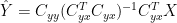
If you agree with Eq.(5) of Tellus, then, by swapping x and y, regressing proxies, x, on temperature, y, yields

G = Cxx1/2 $\Gamma$ xyCyy-1/2

Now you’re seeking a l.s. solution y of

Gy = x,

hence you’re seeking a l.s. solution of

$\Gamma$ xyCyy-1/2y = Cxx-1/2x

Using the pseudo inverse, this is

Cyy-1/2y = $\Gamma$ xy+ Cxx-1/2x

which finally yields Eq.(8) of Tellus:

y = Cyy1/2 $\Gamma$ xy+ Cxx-1/2x

Actually, I like the $\Gamma$ thing, as it really gives the full analogy to the 1-dim case.

Now that I’ve read the other post your equations look right, although I don’t have the time to check carefully. It is clear from above (or your other equations) that the T PCs are linearly composed of the proxies P. Moreover, they are proportional to the inverse P-T (canonical) correlations, given by $\Gamma$ xy+. This is in accordance with your Eq.(19) from the other post as the ssq(cor..) appears in the denominator. No?
Jean S

Posted Jun 14, 2006 at 5:40 AM | Permalink

Gerd, are there (p)reprints of your articles available somewhere — the instutional subscription of my university does not include either GRL or Tellus 😦
Gerd Bürger

Posted Jun 14, 2006 at 6:28 AM | Permalink

Yes, here they are:
Bürger and Cubasch 2005 and Bürger et al. 2006.

But wait: I checked again the $Gamma$ thing in Tellus, and there actually seems to be an error. In Eq.(8) it must read

y = Cyy1/2KyxCxx-1/2 x
with Kyx = Cyy1/2Cxy+Cxx1/2

Obviously, Kyx and $\Gamma$ xy+ are closely related but not identical, and Kyx also seems to posess only singular values > 1 (at least in the examples I checked), which would give the amplification.

Can somebody actually prove this?

Note that this does not affect the simulation results as they are based on the correct formula. But thanks to Steph for auditing!
Steve McIntyre

Posted Jun 14, 2006 at 11:16 AM | Permalink

#18. Gerd, despite your post, I think that your Tellus equation (8) reconciles to your K equation – which should relax you on this point. I’ll post up my reconciliation.

I think that I can now reconcile your Gamma equation to my notation as well; I’m not sure why I had trouble previously. I certainly prefer the C notation for reducing the matrix clutter to how I was doing it. I’m not sure that I prefer the Gamma notation but I’m getting more used to it. Mann mentioned CCA in passing in MBH98 to say that he was unable to get results using CCA, hence his “novel” method.

Another point: because the temperature target series are averages of monthly PC series, they are very close to being orthogonal (though not orthonormal) so the temperature covariance matrix is close to being diagonal (as Jean S has independently observed.) This should lead to a simplification in the canonical correlations using your approach.
Steve McIntyre

Posted Jun 14, 2006 at 11:39 AM | Permalink

The K Equation
$K_{yx} = C_{yy}^{1/2} C_{yx}^{+} C_{xx}^{1/2}$
and
$\hat{Y} = C_{yy}^{1/2} K_{yx} C_{xx}^{-1/2} X$

I.e.
$\hat{Y} = C_{yy}^{1/2} C_{yy}^{1/2} C_{yx}^{+} C_{xx}^{1/2} C_{xx}^{-1/2} X$
$\hat{Y} = C_{yy} C_{yx}^{+} X$
$\hat{Y} = C_{yy} (C_{yx}^T C_{yx})^{-1}C_{yx}^T X$

The Gamma Equation (Tellus)

$\Gamma_{xy}= C_{xx}^{-1/2} C_{xy} C_{yy}^{-1/2}$
$\Gamma_{xy}^+ = (\Gamma_{xy}^T \Gamma_{xy})^{-1} \Gamma_{xy}^T$
$= (C_{yy}^{-1/2}C_{xy}^T C_{xx}^{-1/2} C_{xx}^{-1/2} C_{xy} C_{yy}^{-1/2} )^{-1} C_{yy}^{-1/2}C_{xy}^T C_{xx}^{-1/2}$
$= C_{yy}^{1/2} (C_{yx} C_{xx}^{-1}C_{xy})^{-1} C_{yy}^{1/2} C_{yy}^{-1/2}C_{yx} C_{xx}^{-1/2}$
$= C_{yy}^{1/2} (C_{yx} C_{xx}^{-1}C_{xy})^{-1} C_{yx} C_{xx}^{-1/2}$

Now $\hat{y} = C_{yy}^{1/2} \Gamma_{xy}^{+} C_{xx}^{-1/2} X$
$\hat{y}= C_{yy}^{1/2} C_{yy}^{1/2} (C_{yx} C_{xx}^{-1}C_{xy})^{-1} C_{yx} C_{xx}^{-1/2} C_{xx}^{-1/2} X$
$\hat{y}= C_{yy} (C_{yx} C_{xx}^{-1}C_{xy})^{-1} C_{yx} C_{xx}^{-1}X$

$C_{yy}^{-1} \hat{y}= (C_{yx} C_{xx}^{-1}C_{xy})^{-1} C_{yx} C_{xx}^{-1}X$
$(C_{yx} C_{xx}^{-1}C_{xy})C_{yy}^{-1} \hat{y}= C_{yx} C_{xx}^{-1}X$
$C_{xy}C_{yy}^{-1} \hat{y}= X$
$C_{yy}^{-1} \hat{y}= C_{xy}^{+} X$

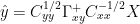
So the K equation and the Tellus equation appear to reconcile OK.
Steve McIntyre

Posted Jun 14, 2006 at 12:13 PM | Permalink

The notation of my earlier post appears to reconcile to Burger’s notation. Having said that, the type of simplification that I did for the one-dimensional case appears to be possible for the multivariate case. Plus the conclusion of the relationship to PLS appears to hold up.

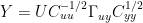
I had written the following expression for the coefficients (U is temperature for me (Bürger’s Y) and Y are proxies for me (Bürger – X). Also I arrange time series by column, Bürger by rows. In my notation:

$G=(U^T U)^{-1} U^T Y$

Using Bürger’s Gamma nomenclature, this is equivalent to :
$G= C_{uu}^{-1/2} \Gamma_{uy} C_{yy}^{1/2}$ where
$\Gamma_{uy} = C_{uu}^{-1/2} C_{uy} C_{yy}^{-1/2}$

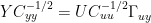
The estimate for the temperature TPCs $\hat{U}$ is derived by the least-squares solution of:
$Y=UG$

Substituting in Gerd’s $\Gamma$ as in his post above, we get:
$Y= U C_{uu}^{-1/2} \Gamma_{uy} C_{yy}^{1/2}$

Thus, in baby steps since blogs are not space-constrained and can do simple steps to ease reconciling,
$Y C_{yy}^{-1/2} = U C_{uu}^{-1/2} \Gamma_{uy}$
$Y C_{yy}^{-1/2} \Gamma_{uy}^{+} = U C_{uu}^{-1/2}$
$\hat{U} = Y C_{yy}^{-1/2} \Gamma_{uy}^{+} C_{uu}^{1/2}$

Allowing for rows and columns exchanging u for y and y for x, this is the same as Tellus (8)
$\hat{Y} = C_{yy}^{1/2} \Gamma_{xy}^{+} C_{xx}^{-1/2} X$

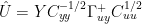
So everything should balance OK. Now let’s unpack the expressions and see how this ties in to the 1-dimensional simplifcation that I’d reported previously:
$\Gamma_{uy}^{+} &=& (\Gamma_{uy}^T \Gamma_{uy} )^{-1} \Gamma_{uy}^T$
$= ((C_{uu}^{-1/2} C_{uy} C_{yy}^{-1/2})^T C_{uu}^{-1/2} C_{uy} C_{yy}^{-1/2}))^{-1} (C_{uu}^{-1/2} C_{uy} C_{yy}^{-1/2} )^T$
$= (C_{yy}^{-1/2} C_{uy}^T C_{uu}^{-1/2} C_{uu}^{-1/2} C_{uy} C_{yy}^{-1/2})^{-1} C_{yy}^{-1/2} C_{uy}^T C_{uu}^{-1/2}$
$= C_{yy}^{1/2} (C_{uy}^T C_{uu}^{-1} C_{uy} )^{-1} C_{uy}^T C_{uu}^{-1/2}$

Now substituting in the equation relating Y and $\hat{U}$ , we get:

$\hat{U} = Y C_{yy}^{-1/2} C_{yy}^{1/2} (C_uy}^T C_{uu}^{-1} C_{uy} )^{-1} C_{uy}^T C_{uu}^{-1/2} C_{uu}^{1/2}$

This yields (before re-scaling):

$\hat {U} = Y (C_{uy}^T C_{uu}^{-1} C_{uy})^{-1} C_{uy}^T$

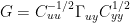
In the one-dimensional case where Y has been standardized to a s.d. of 1, I had said that, if $\gamma$ is the vector equivalent of G (which is $C_{uy}$ here, u is the vector for the single temperature PC and $\rho$ is the columnwise correlation of Y to u, then applying

$\gamma = \rho ||u||^{-1}$ where ||.|| denotes here the standard deviation

$\hat{u} = Y (\gamma^T (u^T u)^{-1} \gamma)^{-1} \gamma$
$= Y (\rho^T ||u|| ||u||^{-2} ||u|| \gamma)^{-1} ||u|| \rho$
$= Y (\rho^T \rho)^{-1} ||u|| \rho$

which was the expression that I had derived previously.

So the algebra ties together to this stage. However, I think that the additional cancellations whon here are worthwhile. The near-orthogonality of $C_{uu}$ has not been used so far. Also this algebra does not show a re-scaling step, which I will derive in a head post.
TCO

Posted Jun 14, 2006 at 12:25 PM | Permalink

Steve:

1. I’m so proud of you. This looks just like all that incomprehensible gobbledigook in the theoretical stats compendium devoted to Hotelling.

2. Is Mann capable of this level of discussion? Have you seen him write papers full of linear algebra?
Steve McIntyre

Posted Jun 14, 2006 at 12:35 PM | Permalink

#23. Is Mann capable of writing “incomprehensible gobbledygook”? What does a bear do in the woods?
Steve McIntyre

Posted Jun 14, 2006 at 12:38 PM | Permalink

I’ve edited the head post to reflect the reconciliation.

The point about PLS was independent of reconciliation issues and appears valid. Now that I’ve reconciled the notation, I’m looking at the variance argument in B-C.
Gerd

Posted Jun 15, 2006 at 2:18 AM | Permalink

Steve, I’m afraid your derivations are incorrect.

#20. You have an incorrect Kyx, with Cyx+ instead of Cxy+. Your Eqs. are impossible simply from dimensioning.

#21. The crucial step is between the following two lines:

Y = UCuu-1/2 $\Gamma$ uyCyy1/2
Cyy-1/2 Y = UCuu-1/2 $\Gamma$ uy

That is invalid. You probably inherited that erroneous conclusion from my earlier post #16. A l.s. optimum is simply not invariant under matrix multiplication (only if the multiplying matrix has the smaller dimensions, seemingly).
Steve McIntyre

Posted Jun 15, 2006 at 6:55 AM | Permalink

#25. So my earlier view that you couldn’t get from A to B seems to be right after all. So if Tellus equation 8 is wrong, I presume that the dimension error that you’ve noted here must have been what caused the original error.
Steve Sadlov

Posted Jun 15, 2006 at 8:09 AM | Permalink

RE: #27 – “Here’s a hint “¢’¬? you idiots can’t audit what you don’t understand!”

Now that is one heck of an egoful statement in its own right. It really reminds me of the archetype of the younger prof, who is trying to carve out his or her territory. Younger profs (I am speaking in terms of what could be biological age, or it could be psychological age) cannot stand it when, say, a TA proves them to be in error, or, comes up with a very creative and new way of doing something resulting in lots of acclaim. The younger prof is seriously threatened by it. That dang ego thing again … what a burden. It prevents constructive work and causes endless pain. Let it go man!
Nicholas

Posted Jun 15, 2006 at 8:37 AM | Permalink

Oh, it’s eminently clear who here is failing to understand…

Steve, and Gerd, keep this up, it’s great! You’re already reaping the benefits of open science. Like they say, “two heads are better than one”.
Ed Snack

Posted Jun 16, 2006 at 3:06 AM | Permalink

It is clear what a realclimatehero is, someone so absurd that they think people discussing results and finding where errors have been made so that ultimately a staisfactory conclusion can be reached is somehow a sign of weakness.

RCH, real weakness is lying, concealing adverse results, and incompetence, all symptoms in full classic display on your “hero” site.
Lawrence Hickey

Posted Jun 29, 2006 at 12:10 PM | Permalink

Dear Blog:
First: can you repeat where the MBH raw data is archived?

Second:
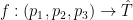
I have a fair grasp of linear algebra, but very limited knowledge of PCA, and through that lens,
I have this idealized- over simplified overview of the reconstruction problem. Help me with any misunderstandings.

Suppose we have three proxys (for simplicity) P1,P2,P3.
Suppose the raw data is a table with 5 column headings, with T being temperature.

[date, P1 ,P2 ,P3 ,T]

The different proxy columns may have different units, Tree ring width might be one example.

Sorting the table by date, most recent first, the temperatures are missing for rows $r > r_v$ . (the reconstruction period).
Take the first m rows, $latex 1 \le r
Lawrence Hickey

Posted Jun 29, 2006 at 12:14 PM | Permalink

(try again) your tex macro didnt like some of my expressions:
First: can you repeat where the MBH raw data is archived?

Second:
I have a fair grasp of linear algebra, but very limited knowledge of PCA, and through that lens,
I have this idealized- over simplified overview of the reconstruction problem. Help me with any misunderstandings.

Suppose we have three proxys (for simplicity) P1,P2,P3.
Suppose the raw data is a table with 5 column headings, with T being temperature.

[date, P1 ,P2 ,P3 ,T]

The different proxy columns may have different units, Tree ring width might be one example.

Sorting the table by date, most recent first, the temperatures are missing for rows $r > r_v$ . (the reconstruction period).
Take the first m rows as the calibration period. Assume we have temperature values for rows in the calibration period.
Rows m
Lawrence Hickey

Posted Jun 29, 2006 at 12:18 PM | Permalink

OK I give up. Here is the latex version- ugly as sin. I replaced the $ sign with the tags but wont work. Looks fine as a latex
document

\documentclass[12pt]{article}
\usepackage{latexsym}
\usepackage{amsmath}
\begin{document}

Dear Blog: \\
First: can you repeat where the MBH raw data is archived?

Next: \\
I have a fair grasp of linear algebra, but very limited knowledge of PCA, and through that lens,
I have this idealized- over simplified overview of the reconstruction problem. Help me with any misunderstandings.

Suppose we have three proxys (for simplicity) P1,P2,P3.
Suppose the raw data is a table with 5 column headings, with T being temperature.

[date, P1 ,P2 ,P3 ,T]

The different proxy columns may have different units, Tree ring width might be one example.

Sorting the table by date, most recent first, the temperatures are missing for rows $ r > r_v$. (the reconstruction period).
Take the first m rows, $1 \le r
Lawrence Hickey

Posted Jun 29, 2006 at 12:21 PM | Permalink

I’m beat. My question is now- what do I need to do to send a valid latex document and not have the site choke on it. Maybe its too long.
TCO

Posted Jun 29, 2006 at 12:31 PM | Permalink

It has problems with the less then sign. Thinks it is a tag.
Lawrence Hickey

Posted Jun 29, 2006 at 1:09 PM | Permalink

again into the breech :

Dear Blog:
First: can you repeat where the MBH raw data is archived?

Second:
I have a fair grasp of linear algebra, but very limited knowledge of PCA, and through that lens,
I have this idealized- over simplified overview of the reconstruction problem. Help me with any misunderstandings.

Suppose we have three proxys (for simplicity) P1,P2,P3.
Suppose the raw data is a table with 5 column headings, with T being temperature.

[date, P1 ,P2 ,P3 ,T]

The different proxy columns may have different units, Tree ring width might be one example.

Sorting the table by date, most recent first, the temperatures are missing for rows $r > rv$ . (the reconstruction period).
Take the first m rows as the calibration period.
Assume we have temperature values for rows in the calibration period.
Rows between m and rv form the validation period which also have temperature values.
Let $(p_1,p_2,p_3)$ be the value of the three proxys for a particular row,

I would think the first job is to find a function f to take an arbitrary $(p_1,p_2,p_3)$ to a temperature.
$f:(p_1,p_2,p_3) \rightarrow \Hat{T}$ .
I would form a m by n matrix A, with n=3, with columns P1,P2,P3. Then form a m by 1 row column vector T from the corresponding m known temperatures
from the raw data table
and solve $Ax \Hat{=} T$ in the least square sense. This means finding the weights vector $x=x_1,x_2,x_3$ such that $Ax=\Hat{T}$
where $\Hat{T}$ is the projection of T onto the column space of A.

With this function f, generated using rows with dates in the calibration period, to examine length of the error vector $\Hat{T} - T$
based on rows in the validation date range, to the that based on rows in the calibration date range.
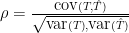
Or we can form the correlation coefficient $\rho = \frac{\mbox{cov}(T,\Hat{T})}{\sqrt{ \mbox{var}{(T)},\mbox{var}{(\hat{T})}}}$
over the validation date range to check that $\Hat{T}$ and $T$ are correlated when we move outside the calibration period
to include validation period dates as well.

Using function f, we can get projected temperatures $\Hat{T}$ for any date in the raw table.
From here draw the graphs of date by f(p1,p2,p3)=T for dates into the reconstruction period as well.
I guess one can use moving averages etc when graphing but thats a detail.

Reconstruction completed.

To get x, one can use either the SVD factorization of $A=U \Sigma V^T$ or use the older method of
$A^T A x = A^{T} T$ which factors positive definite $A^T A$ to get
${(A^T A)}^{-1} = Q {\Lambda}^{-1} Q^T$ . Multiply both sides of $A^T A x = A^T\ T$ by this to get weight vector x.

With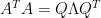 $A^T A = Q \Lambda Q^T$ the eigenvectors are in the columns of Q and the eigenvalues in the diagonal $\Lambda$ ,
one might chop some of the smaller eigenvalues in $\Lambda$ to zero, before forming ${\Lambda}^{-1}$ for more smoothness
but that’s the extent or manual intervention (fiddling) with this approach.

My question is : Where does principal component analysis fit in at all? It seems like its beside the point. How does this help to get function f
that takes us from a proxy row $p_1,p_2,p_3$ to a temperature $\Hat T$ ?

One could process A by taking each proxy column, and subtracting its column mean from each element and dividing by the column variance.
to make $A^T A = R$ into a correlation matrix R, and try to find your factor maxrix F such that $R=F F^T + D$ , D a diagonal matrix
for unassigned variance.
But we introduce the
human element into a selection of how such a factorization is done to account for the all the correlations in R. In recasting R,
(F might be a 3 by 2 matrix in the baby example we cook down the number of proxys to 2) we account for as much of R as we can with a
reduced number of synthesized factors F. But to wnat end?

Please don’t tell me that they take the $F^T F$ instead of A, and use the usual least squares method to construct the weight vector x.
This can’t be what is done by MBH, is it?

Lastly, please explain what the 100 and 200 … year windows are.
I would like to get the actual data and fiddle around with it myself.
Lawrence Hickey

Posted Jun 29, 2006 at 1:11 PM | Permalink

doesnt like \Hat much either does it TCO
wonder if small hat would be better . lets see.
$\hat{T}$
Lawrence Hickey

Posted Jun 29, 2006 at 1:13 PM | Permalink

yup- wants hat not Hat. This thing is a disgrace. Tco can you remove the abortive attempts an I will send it again with small hat. Thanks .
Lawrence Hickey

Posted Jun 29, 2006 at 1:20 PM | Permalink

Tco – can you remove 30-37 and I will post one that works. Sorry.
J. Sperry

Posted Jun 29, 2006 at 1:29 PM | Permalink

LH, that request would be for John A or Steve M. While it’s amusing to consider, TCO doesn’t have that power.
Lawrence Hickey

Posted Jun 29, 2006 at 1:47 PM | Permalink

Ok I’m up for another attempt. Wonder if John A will have mercy on my embarasement trying to get the tex fragments to work
but I’m up for another one. Here goes

Dear Blog:
First: can you repeat where the MBH raw data is archived?

Second:
I have a fair grasp of linear algebra, but very limited knowledge of PCA, and through that lens,
I have this idealized- over simplified overview of the reconstruction problem. Help me with any misunderstandings.

Suppose we have three proxys (for simplicity) P1,P2,P3.
Suppose the raw data is a table with 5 column headings, with T being temperature.

[date, P1 ,P2 ,P3 ,T]

The different proxy columns may have different units, Tree ring width might be one example.

Sorting the table by date, most recent first, the temperatures are missing for rows $r > rv$ . (the reconstruction period).
Take the first m rows as the calibration period.
Assume we have temperature values for rows in the calibration period.
Rows between m and rv form the validation period which also have temperature values.
Let $(p_1,p_2,p_3)$ be the value of the three proxys for a particular row,

I would think the first job is to find a function f to take an arbitrary $(p_1,p_2,p_3)$ to a temperature.
$f:(p_1,p_2,p_3) \rightarrow \hat{T}$ .
I would form a m by n matrix A, with n=3, with columns P1,P2,P3. Then form a m by 1 row column vector T from the corresponding m known temperatures
from the raw data table
and solve $Ax \hat{=} T$ in the least square sense. This means finding the weights vector $x=x_1,x_2,x_3$ such that $Ax=\hat{T}$
where $\hat{T}$ is the projection of T onto the column space of A.

With this function f, generated using rows with dates in the calibration period, to examine length of the error vector $\hat{T} - T$
based on rows in the validation date range, to the that based on rows in the calibration date range.
Or we can form the correlation coefficient $\rho = \frac{\mbox{cov}(T,\hat{T})}{\sqrt{ \mbox{var}{(T)},\mbox{var}{(\hat{T})}}}$
over the validation date range to check that $\hat{T}$ and $T$ are correlated when we move outside the calibration period
to include validation period dates as well.

Using function f, we can get projected temperatures $\hat{T}$ for any date in the raw table.
From here draw the graphs of date by f(p1,p2,p3)=T for dates into the reconstruction period as well.
I guess one can use moving averages etc when graphing but thats a detail.

Reconstruction completed.

To get x, one can use either the SVD factorization of $A=U \Sigma V^T$ or use the older method of
$A^T A x = A^{T} T$ which factors positive definite $A^T A$ to get
${(A^T A)}^{-1} = Q {\Lambda}^{-1} Q^T$ . Multiply both sides of $A^T A x = A^T\ T$ by this to get weight vector x.

With $A^T A = Q \Lambda Q^T$ the eigenvectors are in the columns of Q and the eigenvalues in the diagonal $\Lambda$ ,
one might chop some of the smaller eigenvalues in $\Lambda$ to zero, before forming ${\Lambda}^{-1}$ for more smoothness
but that’s the extent or manual intervention (fiddling) with this approach.

My question is : Where does principal component analysis fit in at all? It seems like its beside the point. How does this help to get function f
that takes us from a proxy row $p_1,p_2,p_3$ to a temperature $\hat T$ ?

One could process A by taking each proxy column, and subtracting its column mean from each element and dividing by the column variance.
to make $A^T A = R$ into a correlation matrix R, and try to find your factor maxrix F such that $R=F F^T + D$ , D a diagonal matrix
for unassigned variance.
But we introduce the
human element into a selection of how such a factorization is done to account for the all the correlations in R. In recasting R,
(F might be a 3 by 2 matrix in the baby example we cook down the number of proxys to 2) we account for as much of R as we can with a
reduced number of synthesized factors F. But to wnat end?

Please don’t tell me that they take the $F^T F$ instead of A, and use the usual least squares method to construct the weight vector x.
This can’t be what is done by MBH, is it?

Lastly, please explain what the 100 and 200 … year windows are.
I would like to get the actual data and fiddle around with it myself.

~

One Trackback

By Abram et al 2014 and the Southern Annual Mode « Climate Audit on Jun 15, 2014 at 10:16 AM

[…] in the AD1400 and AD1000 steps boils down to weighting proxies by correlation to the target (see here) – this is different from the bias in the principal components step that has attracted more […]

Climate Audit