Post Washington, I was browsing through the turgid prose of Rutherford et al 2005 – which actually uses the original MBH98 data set (PC series and all) for nearly half their analysis, they also consider the mystery Briffa et al 2001 sites, which they also do not reveal. The SI says – contact Tim Osborn, which I’ve done with no success. I might as well be talking to a wall – a stone wall.
Mann has used this article to support the claim that he can "get" a HS without PC analyses. Of course, the reason for using PC methods in the first place was to achieve geographical balance – otherwise, people might have been worried that the reconstruction was being overwhelmed by southwest U.S. tree ring data and merely be a local effect. Abandoning PC methods without an alternative summarization allows the bristlecones to dominate the reconstruction through the back door.
Rutherford et al 2005 shows a reconstruction without PCs, which was presented to the House Energy and Commerce Committee. I thought that it would be interesting to compare this to the other reconstructions and, in doing so, noticed something interesting. BTW Jean S has written me offline showing a number of very bizarre and unsupportable aspects of Rutherford et al 2005, which we will pursue, but he’s on holiday and offline for 4 weeks.
The following image plots 4 series from the archived data for Rutherford et al 2005 – combinedannfullnh.txt, multiproxyannfullnh.txt, multiproxypcannfullnh.txt, mxdannfullnh.txt. As you see, the series from 1856 on have a remarkably similar shape; their correlation is exact and, indeed, their values are identical, despite using 4 different data sets. I think that it is a reasonable assumption that all 4 series have grafted instrumental and reconstruction information. Similar results apply to all 15 archived series for Rutherford et al. 2005. The Team are such pranksters.
Figure 1 – plot of 4 reconstructions from Rutherford et al 2005 archived. Red – after 1856.
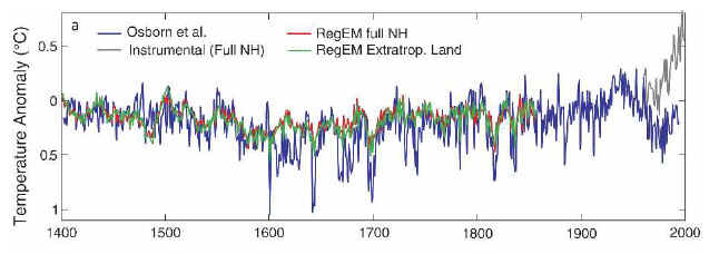
If one consults Figure 2 of the original article shown below, the red in the above diagram looks identical to the grey instrumental series.
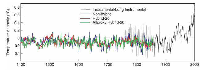
Figure 2 – Figure 2 from Rutherford et al 2005.
Rutherford et al 2005 involved two key lines on the Hockey Team and so the following have archived a graft of instrumental and reconstruction data: Crowley, Rutherford, Mann,Bradley, Hughes, Jones, Briffa and Osboen.
Remember the following Mannian comment at realclimate:
No researchers in this field have ever, to our knowledge, "grafted the thermometer record onto" any reconstruction. It is somewhat disappointing to find this specious claim (which we usually find originating from industry-funded climate disinformation websites) appearing in this forum.
I pointed out such a "graft" for the Crowley reconstruction here. Re-stating Mann’s comment above, would it would be more accurate to say the following? Many of the most prominent researchers in this field have, on occasion, "grafted the thermometer record onto" a reconstruction. It is somewhat disappointing to find the specious claim otherwise (which we usually find originating from the realclimate disinformation website).
Some More Observations
In the top figure, the archived MXD and combined versions, although identical to the MBH98 (pc and all) versions after 1856 don’t end at the same time. The MXD and combined versions end in 1960! (the others end in 1971.) The closing values of the combined reconstruction is around 0 – it does not end on an uptick. The reason for the 1960 termination is the Divergence Problem in Briffa’s MXD series. It trends down after 1960, so it is truncated in most spaghetti diagrams after 1960. Dendroclimatic explanations of the Divergence Factor do not rise above a cargo cult- type of explanation as I’ve posted previously in some detail. Curiously, Rutherford et al inadvertently illustrate the Divergence Problem in a later figure, but do not discuss it.
From Rutherford et al 2005.
When I plotted up the warm-season reconstructions that were archived, I noticed another interesting feature shown below.
Figure 4 – plotted from archived versions at Rutherford et al 2005.
As you see, the post-1856 values are identical in all three reconstructions, but a couple of the series are truncated early. I presume that this is because they didn’t like the results for some reason.


11 Comments
Interestingly, Figure 2 from Rutherford (2005) above is the same graph reproduced in RC’s “Missing piece at the Wegman hearing” post, purporting to show what MBH looks like without PCA. It doesn’t appear to show this at all, even if the “red line” (Hybrid 20) is MBH as they assert in the text.
Jean S has suggested that they meant to post Rutherford’s Fig 3, which would make sense as it includes MBH, and it is “plausible” that it supports their assertion.
I submitted a comment to RC querying this, but of course it didn’t get posted. The nonsensical Fig 2 remains in place at RC. What does it take to get the Hockey Team to concede a mistake?
I don’t pretend to understand RegEM very well. I gather it uses the instrumental period (post 1856) to develop a model that estimates gridcell temperatures prior to 1856. I’ll try to read the paper again to work out what they’ve done. However on this limited understanding, I’m not sure that this constitutes “grafting”. Jean S seems to be up on RegEM – what do you think?
From first impressions, RegEM is like two matrices, one hovering over the other. One is the instrumental temps, one is the proxy data. Then all the missing values are filled in using a minimization function between the two. I think the assumptions must be similar to PCA, eg stationarity, mean values play a big part, or else the results wouldn’t be the same. But then the proxies aren’t significnatly related to local temps, you would get similar results with random numbers, and Rutherford doesn’t use RegEM anyway, e.g. particularly splitting into low and high frequency.
Their method of splitting low-high frequencies is odd to say the least. In signal processing land, we simply take high and lowpass pairs, ala dyadic wavelets or quadrature mirror filters, to create orthogonal frequency banks.
Mark
Steve,
You either have a much better memory than me, a good database, or both. I hate to suggest more work, but do keep a sort of “pending request file” with date, name, study, periodical, nature of request, result and links to other relevant information?
I don’t think it would make you many friends to show on line all requests, but a page showing those long overdue a reply would make a good role of shame and might well throw light on the way some of the social networks work.
Would sure like some feedback on my favorite reconstruction (the article in Ecological Modeling).
“Oh what a tangled web we weave,
When first we practise to deceive!”
Sir Walter Scott, Marmion, Canto vi. Stanza 17.
Scottish author & novelist (1771 – 1832)
jae – Would sure like some feedback on my favorite reconstruction (the article in Ecological Modeling).
Interesting stuff.
But what I noticed more from the data was that there is another extreme cooling period that we seem to have forgotten about, “The Dark Ages.”
It is generally recognized that civilization fell apart in the years 350 AD to about 650-850 AD and one of the biggest reasons was the extreme cooling that Europe
(at least) experienced.
The climate models do not explain the climate variation of the past 2,000 years. They do not explain the climate variation of the last 7,000 years. They do not explain the climate variation of the past 3.0 million years of ice ages and interglacials.
Obviously, they do NOT work. Simple greenhouse gas accumulations do not explain the climate adequately, except for perhaps the past 150 years. Now that used to be called a “spurious explanation”, an explanation that just by chance works but is either:
– illogical to start with (not really in the case of greenhouse gases since there is some theory and logic to it); or,
– entirely accidental (since global warming is certainly not proven yet we should accept this alternative as possible): or,
– by chance the variable(s) only work some of the time and do not explain all of the variation which needs to be explained (which is by far the most likely alternative.)
This is why Mann’s “hockey stick” was so important to the AGW crowd. They needed to remove the spurious relationship that exists for the past 150 years and extend it as far back in time as possible.
They need to build (much) better models that can explain the climate variation of the past 400,000 years and especially the last 11,000 years before we can say they have adequately proved anything.
Re#5 I like the emphasis of a “Dark Ages” cold period.
I believe that the Northern European frontier of the Roman Empire was the River Rhine. For many years the Romans had a large fleet of ships on the Rhine to prevent undesirables from crossing it into the Imperial territory.
Late in the Empire the story goes that one year, 31st December 406, there was particularly severe winter, and the Rhine froze solid, a very unusual event. The various tribes took the opportunity to cross the Rhine en masse in wheeled vehicles. Thus the end of Roman control over that section of their Empire.
See also “What do we know about the Dark Ages Cold Period as it was experienced in Europe?”
Link
Yes, it indeed is. To be exact it is HadCRUT grid cell temperatures for NH up to 70N infilled with RegEM (see Rutherford, section 2a). They infilled the instrumental grid cells with RegEM BEFORE using any proxy data. These infilled intrumental temperatures are used for verification, this is a problem noticed by B&C (“verification bias”).
#8
Mark I heard a number of anthropologists blame an abrupt cooling in Northern and Central Europe led to the demise of Rome as much as anything else.
I’ve always wondered why this period isn’t studied more from a climate point of view. Was the cooling local, or more widespread? Can precipitation proxies point to any draughts? How much did the NAO play in this cooling? Just a thought.
#10 this is the kind of antedotal evidence you are thinking about. This book blames Krakatoa for the fall of the Roman Empire