Paul Linsay continued his look at the statistics of hurricanes by looking at the entire record, which I present here:
I went back and repeated the analysis for the Atlantic hurricane data but this time used all the data back to 1851. There is some question about undercounts prior to 1944 but I ignored that issue and used the data as is. The principal change is that the mean number of hurricanes dropped to 5.25 per year from 6.1 for the period 1944 – 2006. The plot of the yearly counts again looks trendless ( Figure 3).
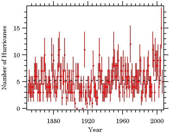
Figure 3. All hurricane counts from 1851 to 2006. The dashed line is the mean of 5.25 hurricanes per year.
The distribution of counts and a calculated Poisson distribution with an average of 5.25 are plotted in Figure 4. The error on the bin height, sqrt(bin height), is also plotted. Just like the 1944 – 2006 data, there is good agreement between the two.

Figure 4. Histogram of annual hurricane counts(red), 1851 to 2006 and associated Poisson distribution(blue). The errors on the bin heights are plotted in black.
Once there are a large number of events it becomes possible to start looking for rare events predicted by a Poisson distribution. With an average of 5.25 hurricanes per year and 156 years of data the probability is high that there will be at least one year with no hurricanes. This is calculated as follows. The probability of no hurricanes in a particular year is exp(-5.25) = 5.2e-3. In 156 years we then expect 156*exp(-5.25) = 0.82 years when there were no hurricanes. Referring to Figure 3, there were no hurricanes observed in 1907 and 1914.
Poisson processes also have the property that the time interval, T, between events is distributed as C*exp(-T/T_o) where T_o and C are constants. (See for example, L. G. Parrett, Probability and Experimental Errors in Science, Dover, 1971).
Using the Atlantic data that SteveM archived here I computed the time in days between hurricanes for all the data from 1851 to the present and histogramed the time differences. The result is in Figure 5.
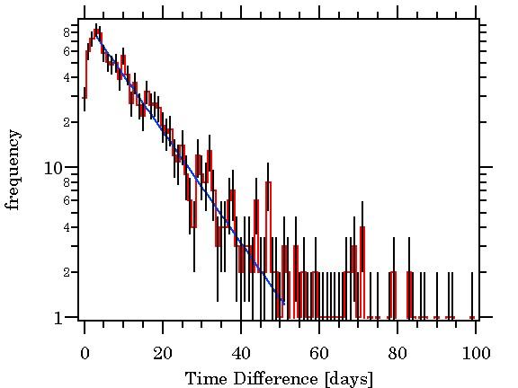
Figure 5. Histogram of the time interval between hurricanes, semilog plot. The distribution is in red, the error bars are plotted in black, and the best fit exponential is plotted in blue.
It is quite obvious from the plot that the time intervals are distributed exponentially for intervals between 3 and 51 days. There is a deficit for time intervals shorter than three days, probably due to physical limitations of hurricane formation. There is also a very long tail beyond 50 days.
I performed a least squares fit of the distribution to an exponential using sqrt(bin height) as the one sigma error (Poisson!). The result is the blue line in the plot with a time constant, T_o, of 11.6 +- 0.5 days. Overall, the chi-square was 47.5 for 47 degrees of freedom(49 data points – 2 parameters), a very good fit.
The evidence seems quite clear that hurricanes are the result of a stochastic process that obeys Poisson statistics. The annual counts are distributed as a Poisson distribution and matches the distribution computed from the average of the annual counts. Rare events, years with no hurricanes, are seen at a rate predicted from the distribution properties. And the time between hurricanes follows an exponential distribution.
A final note: If I were to do more analysis of hurricane counts I wouldn’t do a global analysis but group them by area of origin to see if 


117 Comments
Here’s my amateur, impressionist view: it looks like the undercount of earlier years is causing a deviation from the Poisson curve, dampening the number of expected hurricanes.
My long term prediction stands: 6 +-3 hurricanes per year.
I wonder what William Gray makes of this analysis…
May I suggest that CA creates a bibliography page on which the regular statistical posters can recommend books about the statistical methods being used?
rwnj:
Since R is used here alot, I have found the two books listed below useful, plus the turorial matertial at the r-project web site. Look for the link on this page under Stastistics and R. (Upper left).
Using R for Introductory Stastistics, John Verzani, Chapman & Hall/CRC
R Graphics, Paul Murrell, Chapman & Hall/CRC
These two books and the turorial material have allowed me to gain some statistical insight, and to down load data files and plot the results. I am still struggling with some of the complex math, but learn more everyday that I visit here. I have down loaded some of Steve M. scripts and decoded them. It takes a while, but very interesting to get one working and then tinker with the filters and plot the different results.
To Paul Linsay and John A, I say good work in calculating and publishing the fit of the NATL hurricane counts to a Poisson distribution. My only complaint is that of using the annual count only to produce the error bars. You have established a Possion distribution with mean of 6.1 (initial thread) and 5.25 (this thread) using all the available annual results for the time period of interest. Use the standard deviation derived from this excercise to produce the error bars for the annual data points, i. e. the square root of the mean.
You have 2 data points with 0 annual counts in the lead-in graph and you have error bars or the lack of indicating 0 error. Now if I had run this test on Mars and for 63 or 100 plus years and I never counted a hurricane I would have a mean of zero and error bars showing 0 error — but not on earth — in the NATL.
You cannot conclude that hurricanes numbers are a Poisson process with a constant mean from these analyses.
First you need to check the goodness-of-fit between the data and the expected distribution. There are several ways of doing this, a Chi-squared test is simplest, but there are probably more powerful tests.
Second, you need to test the statistical power of your analysis. What would the distribution would look like if the mean varied, perhaps between 4 and 8 hurricanes per year. Does this distribution still appear to be a Poisson process? If it does then this discussion is a type 2 error.
I fret about commenting here (on the site) because I am NOT terribly conversant in a lot of the
statistical methods (I went to grad school in political philosophy for crying out loud), but I
have been looking at this same data for a while now. I’ve reached some conclusions, based upon
my admittedly limited knowledge, but I’d like to know what folks think I’ve done right or wrong,
and where the weaknesses of my understanding lie.
OK, so we are looking at tropical storm/hurricane formation in the Atlantic basin in an historical
perspective. Based upon the caveats included in the NOAA historical data set, I decided to limit
my investigation to the 1946-2005 time period. (It also makes for an even 60 year period.)
So I’ve loaded up my data onto a spreadsheet and found the following basic statistics:
# of Tropical Storms 634 (avg. 10.5667/year)
# of Hurricanes 369 (avg. 6.15/year)
Next, I get the standard deviation for the T. Storm number ang get back a value of 3.9504
(and for just hurricanes a values of 2.5765)
Even I know these are very large numbers, so I look around for reasons (thank you google) and I
hit upon the possibility I could be looking at a lognormal distribution. Is this reasonable? I
think it is, but I’m open to being convinced otherwise.
In any event I get log10 values for the data, and get
mean: 0.9971
standev: 0.1533
extrapolating the numbers back out (i.e. 10 ^ 1.1504) I get an upper value of
14.1372 storms, with a mean (i.e. 10^0.9971) of 9.9334 storms. This makes the
lower boundary 5.7296. OK so I look at how much of the original data falls
between 6 and 14 inclusive. I find 51 out of 60 (85%) observations fall in that range.
So once again that looks pretty good, or I’m not seeing anything that argues agaisnt this being a lognormal distribution. I think.
Anyway, I was doing all of this because of the news story about RMS downplaying
most of the historical data and stressing the last 12 years. The argument seems
to be that the last 12 years were so unusual, in term of tropical storm activity, that
it must be indicative of new rules to the game.
So I looked at the 12 years 1994-2005. Using the log10 numbers I get a mean of 1.1354,
for that time period which seems to be within ONE standard deviation of the 1946-2006 values.
(i.e.,0.9971+0.1533=1.1504)
That is about as far as my limited knowledge can take me. Where have i screwed up,
what dont I know?
richardT, regarding the excellent point raised in your post, I have posted on this question here.
All the best,
w.
Re: #5
RichardT, I did a chi square goodness of fit test for the data above for 1851 to 2006 using a Poisson distribution and mean of 5.25 and found that the probability of a fit is very low.
I then did a chi square goodness of fit test on the original data used by Paul Linsay in the initial post, using a Poisson distribution with a mean of 6.1 and found a very high probablity of a fit.
I can do more analysis tomorrow but bed beckons now.
I don’t want to talk about those error bars anymore, time to move on;)
We still have the issue with ‘explains 76 % of the variance’. So how about testing a model HCount ~ Poisson(a+b*SST) . Would that be silly? For example, with Matlab
HCsim=poissrnd(ones(151,1)*5.25+k*SSTs);
where SSTs is standardized SST. Test with different k’s and try (many many times)
corrcoef(SST,HCsim)
corrcoef(M*SST,M*HCsim)
where matrix M does the 9-year averaging trick.
And then model the measurement errors with another Poisson process. How sensitive the results are wrt measurement errors? What k gives closest reported values for the correlations? Or is k zero? Try both hurricane count and TC count.
One of the persistent questions in all of this is the quality of the storm count data: are the records good enough to allow comparisons between today and earlier years?
There’s a general belief that, post 1944, the storm count data is good. I’m not so sure about that.
Here are some numbers, looking at peak periods of Atlantic activity:
Tropical cyclones (1945-1954): 10.3 per year
Tropical cyclones (1995-2004): 13.6 per year
(Significant jump.)
But, there’s something odd when one looks at those storms which were easily detectable (came within 100km of land) and those that remained at sea and were thus harder to detect:
Tropical cyclones within 100km of land (1945-1954): 7.9 per year
Tropical cyclones within 100km of land (1995-2004): 8.2 per year
(Almost identical counts.)
Tropical cyclones which stayed at-sea (1945-1954): 2.4 per year
Tropical cyclones which stayed at-sea (1995-2004): 5.4 per year
(Big jump in the harder-to-detect storms.)
So, the “regime increase” was in the harder-to-detect storms, not in those near land. Odd.
But surely there were aircraft patrolling the far reaches of the Atlantic, etc. Well, here is some information from a 1961 book (“Atlantic Hurricanes” by Dunn/Miller, who were specialists. One was the hurricane center director):
* even in the late 50s, 50% of cyclones were still first detected by ships, not aircraft
* shipping lane detection was important. get away from the lanes and data drops.
* the only patrol mentioned consisted of a flight from Bermuda to east of St. Croix and then towards Miami and back to Bermuda – sort of a Bermuda triangle route. What about the vast ocean east of the Antilles?
I, and maybe Occam, suspect that storms, especially weak and more-remote ones, were missed before satellite coverage became good in the 1970s.
I tried using a range of Poisson means for the chi square goodness of fit test as completed above for the time period 1945 to 2006 with a 6.1 mean (the 1851 to 2006 distribution with a 5.25 mean was eliminated from this exercise since the probablity of the differences between its distribution and a Poisson happening by chance is greater than 95%). Using the 95% limit again, I found that the differences for Poisson distributions with a range of means from 5.5 to 7.2 would pass the chi square goodness of fit test for the actual numbers derived from the data originally used by Paul Linsay (that had the 6.1 mean for the 1945 to 2006 period).
I would suggest that the data (time period) used in the 1851 to 2006 be split into that used initially by Paul Linsay (with 6.1 mean for the period 1945 to 2006) and the time period prior to that one (1851 to 1944) and then used to calculate separate Poisson means.
I would guess that by combining the data we are looking at the combination of at least 2 Poisson distributions with differing means. We suspect that the earlier data contains under counts and if these under counts occurred randomly we could expect to see a Poisson distribution — just one with the lower counting efficiency contained in a lower mean.
If that counting efficiency varied considerably in the 1851 to 1944 period, I would suspect that a single Poisson distribution and mean would not show a good fit with the resulting distribution.
I believe I have the data to do all this but will not have time until later as a higher authority has requested my time at the moment.
I split 1851 to 2006 data into two parts: 1851 to 1944 and 1945 to 2006. I obtained a mean hurricane occurence for the 1851 to 1944 time period of 4.96. A chi square goodness of fit test for the distribution being Poisson with a mean of 4.96 showed no fit to a Possion distribution. Probability of the distribution from 1851 to 1944 being Poisson was 0.3%.
I recalculated the mean occurence for the period 1851 to 2006 and obtained 5.48 and not the reported 5.25. Using that mean value and a Poisson distribution in a goodness fit test showed that this distribution does not fit a Poisson distribution either.
As I stated earlier, this non-fit prior to 1945 may be caused by a significant changing hurricane count efficiency during that period. It might be of interest to further split the 1945 to 2006 data in half, but then the number of data points may well be too small to get a statistical measure of the goodness of fit.
Ken,
I don’t know how you computed chi squared for the distribution nor have you quoted your numbers. You have to provide more details so that we can understand what you did.
I computed a chi square of 22.2 for 16 degrees of freedom which corresponds to a CL of 0.14, not great but good. The correct method for computing chi square for Poisson statistics and a histogram are given by equation 32.12 here with a complete explanation of the derivation in S. Baker and R. Cousins, Nucl. Instrum. Methods 221, 437 (1984) available at
“http://ccdb4fs.kek.jp/cgi-bin/img/allpdf?198311266”
The result is derived from a maximum likelihood that uses the Poisson distribution directly. Should the data be split into pre and post 1944? Maybe, but I don’t think it’s necessary based on the chi squared fit.
RichardT and Willis, statements like
are infinite in number. I refer the simplest explanation, Poisson. There are three pieces of evidence for Poisson statistics with a single mean for all the data: the distribution of annual counts is well matched by a Poisson distribution computed from the mean and the number of samples; simple Poisson statistics predicts at least one year with no hurricanes, which is observed; and if this is a Poisson process, the time intervals between hurricanes should be random and distributed as an exponential, which they are.
UC, what’s the point of trying to correlate a random series with SSTs?
As a former industrial analytical chemist, I see the time series plot of annual hurricane numbers in terms of a Shewhart control chart, specifically a C chart. As such, it seems clear to me that the process depicted is not in statistical control, i.e. not random or at least not well described by a simple Poisson distribution, because of the several long runs above and below the mean. As I remember, a single run of about 8 above or below the mean is sufficient to declare a process “out of control”. That’s the rule for X-bar charts, I’m not sure if it is the same for a C chart, though. If I were really motivated, I’d try to plot a CUSUM chart for the first figure. Anybody have a stat package that will do that?
Not sure what you mean by random series, but k surely affects the distribution of sample correlation coefficient (SST from natldata.xls, SSTs = standardized SST) :
k=0;
R=zeros(1000,1);
for i=1:1000
HCsim=poissrnd(ones(151,1)*5.25+k*SSTs);
r=corrcoef(SST,HCsim);
R(i)=r(2,1);
end
mean( R )
ans =
-0.0011
std( R )
ans =
0.0847
% set k=1
k=1;
R=zeros(1000,1);
for i=1:1000
HCsim=poissrnd(ones(151,1)*5.25+k*SSTs);
r=corrcoef(SST,HCsim);
R(i)=r(2,1);
end
mean( R )
ans =
0.3999
std( R )
ans =
0.0659
%(But I’m more interested how measurement errors affect these, both SST errors and under-counting)
RE: #14 – Ironically, although it has a lot in it, I can’t seem to find a CUSUM in my StarSigma pull down. I would personally be very interested in seeing a CUSUM of this. Anyone? Thanks in advance …
I plotted the data for NATL hurricanes in Excel using what I think is the correct formula for Cu Sum or CUSUM (summation of observation minus target) from 1851 to 2006. There are clear, relatively long term changes in the target from 1851 to 1994, but the range is from about 5 to 6. Things change in 1995 though. There is a clear break upward and the new target level is about 8. Not coincidentally, I think, 1995 is when the satellite Arctic temperatures start rising rapidly. I would post the chart if I knew how.
Re: #13
Paul, I used the standard chi square goodness of fit test for a Poisson distribution as shown in “Statistics for Businees and Economics” pages 437-442. I used the actual number years for a given hurricane count, (Oi) and compared it with the expected number of years for given hurricane counts using the Poisson distribution with the calculated mean (ei).
Then chi square = Sum from i=1 to k (Oi-ei)^2/ei
I also used the bin rule of combining bins when the number in a bin was less than 5 and I also used k-2 for the degrees of freedom. Doing this gives degrees of freedom less than what you noted. The results were as follows:
1945-2006:
Mean = 6.1, df = 6, p = 0.965
1851 to 2006:
Mean = 5.48, df = 10, p = 0.006
1851 to 1944:
Mean = 4.96, df = 7, p = 0.006
Let’s see if this works:
Wow, it does.
The above chart uses a target level of 5.0 storms/year.
Also the target range for 1851 to 1994 is more like 4 to 6 if I include the data from 1900 to 1932. I hope this doesn’t put me over the limit for the spam filter. Comment editing???
DeWitt, a bit off-topic, how did you go about getting your plot to post? I’d like to learn that process. Thanks
Copy chart to Paint. Save as JPEG. Upload to free online image hosting site like Yahoo Flickr. Get the URL of the image from the hosting site and use the Img button to include the URL of the image in the message. For more details, see the last answer here.
Re: #14
The Shewhart control chart would show a plot of the data points against 3 lines representing the mean and +/- 2 standard deviations. For a Poisson distribution this would be the mean and +/- 2*mean^1/2. The CUSUM charts are used to show a changing mean before the change represents 2 standard deviations. These charts are typically used assuming that the distribution is normal.
The trends identified by the CUSUM chart derived from the hurricane data, I think, would represent the cyclical and/or auto correlated features of the data. If there is a large cyclical and/or auto correlated component in the the 1945 to 2006 hurricane count it is surprising, to me anyway, that it would give such a good fit to a Poisson distribution with a mean of 6.1. It would appear that the actual case could represent the combination of more than one Poisson distribution, i.e. more than one Poisson mean. I’ll need to look at this in more detail — unless, of course, someone at this blog can enlighten me.
Re: #24
Classic Shewhart like X-bar and R charts assume normality but use +/- 3s for the upper and lower control limits. Otherwise you get too many false alarms. You may also see 1s and 2s lines if you use the Western Electric control rules which includes runs above and below the mean, consecutive monotonic runs and too many points outside +/- 2s. However, all these extra rules increase the probability of a false alarm from about 3/1000 points to about 1/100.
The C attribute chart, however, is for Poisson distributed data (number of defects per time period, e.g.) and as a result may not have a lower control limit because it would be less than zero. The upper control limit is not as well defined either. A CUSUM control chart uses a V mask for control limits and finds small changes in processes (0.5 to 2s) faster than a simple attribute chart. I couldn’t find much information about a CUSUM C attribute chart so I’m sort of winging it. For more details about CUSUM charts in general, see for example here.
I plotted various subsets of the hurricane data and the 1944 to 2006 data has a long run from about 1951 to 1994 where the target value doesn’t appear to change much (about 5.5). So I’m not at all surprised that a Poisson distribution gives a reasonable fit.
#13
As I am sure you are aware there are two types of statistical errors: Type 1, to incorrectly reject the null hypothesis; and Type-2, to accept the null hypothesis when it is wrong. Type-2 errors generally occur when the statistical test lacks power, either because there are few data, or the test is inefficient.
One of the simplest ways to test the power of an statistical test is by simulation – generate datasets where Ho is false and see if the test rejects Ho. This is what I have suggested.
The use of a test with little or no statistical power is a rhetorical device, not science.
Re: #26
RichardT, what you say is correct, but in this case if you look at the p values for the three cases where I did the goodness of fit tests you will see that for the time period 1945 to 2006, p = 0.965, while for the 1851 to 1944 and 1851 to 2006 time periods, p = 0.006. The acceptance level for a fit is normally used as p =/> 0.05. This would tend to indicate that one has to measure rather significant deviations before rejecting the hypothesis that there is a fit. In this comparison, however, the probabilities are very different and show that the 1945 to 2006 period has a very much better fit to a Poisson distribution than the other periods. That allows us to look for the causes of these differences.
It is important also to remember that the goodness of fit chi square tests uses the statistic [observed value (Oi) — the expected value (ei)]^2/ei and that number gets very large when you have relatively large observed values, Oi, where the distribution being measured calls for small expected values, ei. For example, tails extending toward zero expected values that show significant actual values has a very large proportional weighting of the chi square test against a significant fit. Since those numbers approaching zero in smaller samples also tend to have bins that have to be combined, the binning technique becomes important.
In addition, using a range of means for the Poisson distributions as I completed in an earlier post shows by comparison that as one increases or decreases the distant from the 6.1 mean for the 1945 to 2006 period that the probability (p) in the goodness of fit test changes dramatically. When one uses a p =/> 0.05 go/no go limit this is less evident.
Re: #25
You are correct about those control limits. Talk about type II errors. I think I have a mental block on that going back to my days dealing with manufacturing processes and trying to educate a work and support force about the need for establishing more process capability from the get go and having to spend less time adjusting the process. It brought back memories of changing the sampling mentality and cultural inertia for the times when 1 and 2% product rejects were considered acceptable to the times when 0.1% was no longer acceptable. Those old product sampling plans with their huge Type II errors were no longer practical for the higher quality product demands and brought home the message that quality could not be “inspected” into the product.
RE: #25 – I use CUSUM to identify a superset of potentially actionable stuff but not as a general alarm basis. It’s handy for identifying abnormalities of an unknown nature. Then you root cause the abormality (or set of them) to determine the actionable subset. Based on my own operational philosophy, the little “mini run” of ~8 data points would warrant further study to understand what if any causals might be gleaned.
Re: #18
I went back and checked all my calculations using the original Landsea data plus 5 hurricanes for 2006 and 15 for 2005 and obtained the following corrected results for the means and probabilities for the chi square test for goodness for fit to a Poisson distribution:
Mean = 6.1, df = 6, p = 0.974
1851 to 2006:
Mean = 5.25, df = 8, p = 0.087
1851 to 1944:
Mean = 4.69, df = 6, p = 0.416
These results would have all 3 distributions passing the goodness of fit test, albeit for the period 1851 to 2006, barely. The tails towards zero expected events and binning selections can produce large differences in the resulting values of p.
The poor fit for the combined data may be the result combining two different Poisson distributions made so by way of significanlty differing Poisson means. An explanation, that no doubt oversimplifies all that is occurring here, might be that we are looking at two Poisson means differing by the under counts between periods 1851 to 1944 and 1945 to 2006. That is not to say that other effects are not operating here such as changing counting efficiencies within these periods and cyclical tendencies.
Re: #13
I feel that I should explain in more detail the errors I made in making my initial calculations of the chi square goodness of fit. First of all I do not want to imply that any of the graphical presentations made by Paul Linsay were in error. Linsay’s graphical presentations were correct in all manner. The errors made were mine alone and for that I apologize for any misleading conclusions that might have resulted from them.
My errors were in adding one hurricane to each of the counts for 13, 14 and 15 hurricanes for the 1881 to 2006 and 1881 to 1944 time periods. Hurricanes, with the means of those periods, would have very low expected frequencies in a Poisson distribution for those numbers of hurricanes i.e. 13, 14 and 15. The counts should have been 0, 0 and 1, for the 13, 14 and 15 number of hurricanes, respectively.
Just to illustrate how rare the predicted occurrences are for these numbers of hurricanes in a Poisson distribution we have for the means of 6.1 and 5.25:
For a mean of 5.25 we would expect 15 hurricanes in a year to occur every 3900 years and similarly for 14 hurricanes every 1374 years and for 13 hurricanes every 515 years.
Doing this for a mean of 6.1 gives 15 hurricanes every 968 years; 14 hurricanes every 394 years and 13 hurricanes every 171 years.
Using these same numbers can illustrate the effects of binning that are required in doing a chi square goodness of fit test. We would not bin to obtain a count of 1 (the rule requires a minimum of 5) but the point can be made nevertheless. If we binned all the counts of 13 hurricanes and greater we would derive the following expected occurrences for 13 or more hurricanes:
For a mean of 5.25 we would expect 13 or more hurricanes every 342 years and for a mean of 6.25 we would expect 13 or more hurricanes every 106 years.
If one assumes a Poisson distribution with a mean of 6.1, 2005 was truly an unusual year with 15 hurricanes — in fact a once in a thousand year event. If we consider it a 13 hurricane or greater occurrence then it was a once in a 100 year event.
Looking at it another way, to obtain an expected occurrence of 1 year with 15 hurricanes in 156 years, assuming a Poisson distribution, would require a mean of approximately 7.6 hurricanes per year.
In #31 above, the Re: #13 should read Re: #30
In an effort to complete what I started here, I did chi square goodness of fit tests for the distributions from the same time periods as these tests were run previously for a Poisson distribution. This time for a fit to normal distributions. The fits were not as good as they were for a Poisson distribution, but using the standard 0.05 limit a fit was found for the 1945-2006 and 1851-1944 time periods. The results are listed below:
1945-2006: Mean = 6.10, Stdev = 2.57 and p = 0.878.
1851-2006: Mean = 4.96, Stdev = 2.36 and p = 0.166.
1851-2006: Mean = 5.25, Stdev = 2.53 and p = 0.001.
Just to show that the chi square goodness of fit test cannot distinguish between a Poisson and Normal distribution with relatively large numbers of counts, I did a goodness of fit test of the 1945-2006 using the expected values from a Poisson distribution with a mean of 6.10 and tested it for a fit to a Normal distribution with a mean of 6.10 and a standard deviation of 2.57. The probability of a fit was p = 0.999.
I also looked at autocorrelations for AR (1) and ARMA (1,2) for the time series from 1851-2006 by simply doing the regressions (and not by doing a Box-Pierce or D-W test) and in both cases the R^2 values were approximately 0.025 which indicates to me that little autocorrelation exists.
#33 This may be covered and you already may know this but a poison distribution is pretty much identical to a normal distribution for a relatively large number of counts. A poison distribution for a large number of counts is pretty much a normal distribution where the mean equals the standard deviation.
http://en.wikipedia.org/wiki/Poisson_distribution
John, as you likely know, this depends on lambda, and is only true for large lambda. For a small value of lambda, where there are a number of counts of zero, the distributions diverge.
w.
Re: #34
Yes and that is why I wanted to show that while you can pass the goodness of fit test for some time periods with both a normal and a Poisson distribution, the fit with a Poisson distribution was better in all cases.
Re: #35
You make a good point and a small part of the poor fit for the the 1851-1944 time period (with a smaller mean/lambda)with a normal distribution results from a normal distribution allowing negative counts while a Poisson distribution and the actual one cannot go negative.
Using a stdev that is reduced with the square root of the mean (as opposed to using an unchanging stdev) for a normal distribution keeps the fit between a normal distribution and Poisson “fitting” as the means (lambdas) are reduced, but with means less than 4, the divergence between the normal and Poisson distributions is rapid.
There are a number of very interesting papers on arXive at the moment, including:
From the paper on the comparison between IPCC models and simple statistical methods, their conclusions:
4 Conclusions
We are developing methods to predict hurricane numbers over the next 5 years. One class of methods
we are developing is based on the idea of predicting main development region SSTs over this time
period, and then converting those predictions to predictions of hurricane numbers. Hitherto we have
used simple statistical methods to make our SST predictions. In this article, however, we have considered
the possibility of using climate models instead. We have compared predictions made from an ensemble
of state-of-the-art climate models with our statistical predictions. Climate models that include a perfect
prediction of future volcanic activity are the best predictions of those that we consider. Climate models
that ignore volcanic activity, but include a perfect prediction of other climate forcings, do very slightly
better than our statistical models up to a lead time of 5 years, but do increasing less well thereafter. Given
the unfair advantage that using perfect predictions of future atmospheric forcing parameters confers on
the climate models, the tiny margin by which they beat the statistical models, and the vast complexity
of using these models versus using the statistical models, we conclude that the statistical models are
preferable to the climate models over our time period of interest.
We have thus answered our initial question. Should we use IPCC climate model output to feed into our
predictions of future hurricane numbers, rather than the simple statistical methods we currently use?
The answer is no.
What can we say about (a) whether the climate models might one day be preferable to the statistical
models and (b) what this tells us about predictions of climate in the 21st century? Wrt (a), the one
obvious way that the climate model predictions might be improved would be to include realistic, rather
than random, initial conditions. If there really is a component of unforced internal climate variability
that is predictable on decadal and interdecadal time-scales, and the models can simulate it, then their
errors might be reduced. However, whether predictable internal climate variability exists on these long-
timescales is currently unknown, and climate scientists have different opinions on this sub ject. In the
absence of such signals, at short lead-times both the statistical models and the climate models are probably
hitting the limits of predictability defined by the levels of interannual variability in the climate, that is
unpredictable over the time-scales of interest. At long-time scales it seems likely that the climate models
could be significantly improved, by the gradual eradication of the slow drift that is presumably driving
the more rapid increase in the climate model errors versus the errors in the statistical model.
Wrt (b), should we extrapolate these results to tell us about the likely skill of future climate predictions?
This is rather hard to answer, since it depends, in part, on what the climate does in the future. But,
prima facie, the suggestion from these results is that statistical models will continue to do as well or better
than climate models in the future. However, what if future climate variability is dominated by single
externally-forced upward trend, as many climate models suggest, rather than by interdecadal variability,
as it has been in the past century? Will the climate models then do any better? Perhaps. Although
at that point statistical models that capture trends would improve as well, and the comparison between
statistical models and climate models would have to be repeated.
re: #37
I know what they mean, but it’s still funny to consider a climate model which could make perfect predictions of future volcanic activity. Almost as funny as the IPCC or the Team.
While browsing I came across this reply posted on Roger Pielke’s website which i simply want to record here, so that I don’t forget it:
We shall see. I believe their initial forecast comes out about in about five weeks.
IT’s interesting that Judith refers here to the June 2006 ECMWF forecast. Last August and September, I tried very hard to get this prediction from both Webster and Curry without any success.
http://www.climateaudit.org/?p=790#comment-43120
http://www.climateaudit.org/?p=790#comment-43168
http://www.climateaudit.org/?p=790#comment-44429
Now that the season is over, once again their prediction materializes. I wonder why Curry and Webster seemed to have so much trouble locating it in August and September.
That’s the nature of climate prediction. You only do it after the event to show how good your modelling was.
Since this thread has become active again I thought I would add a bit more analysis.
There was some discussion of whether there is an undercount of hurricanes prior to 1944, an increase of hurricane activity in the late twentieth century, or a sinusoidal modulation of the mean number of hurricanes. While one or more of these is possible the variation in hurricane counts over the entire period back to 1851 can be explained by another application of probability theory, random walks. Random walks come about in many situations: the gambler’s ruin problem, diffusion and Brownian motion, and stock market time series are a few examples.
In the classic one dimensional random walk, a marker is placed at zero and then moves +1 if a coin flip comes up heads, and moves ‘€”1 if the coin comes up tails. The coin has a probability p of coming up heads and probability q = 1-p of coming up tails. It can be shown that after N coin flips the mean position of the marker is N(p-q) +- sqrt(4Npq). The recurrence time T_00 is the time between successive visits to zero. It turns out that the mean of T_00 is infinity. Taken together, these facts explain the behavior of a random walk, which is not intuitive. The marker does not dither around zero but spends long periods away from zero because the walk is made up of strings of mostly heads alternating with strings of mostly tails. Plot several for yourself with N = 10,000, you’ll see the long excursions away from zero.
It explains the gambler’s ruin. Suppose you play a game where you win a dollar on heads and lose a dollar on tails with a fair coin, p = q = 1/2. If you have a small bank roll and your opponent has a big bank roll, you will always lose because eventually one of those strings of mostly tails will come along and wipe you out, while he can wait out the strings of mostly heads. Casinos understand this extremely well.
For the hurricane counts, define heads as any year with five or fewer hurricanes and tails as any year with six or more hurricanes. For a Poisson distribution with a mean of 5.25 it is easy to calculate that p = 0.57 and q = 0.43 meaning that hurricane counts form a biased random walk. The apparent early year undercounts and later year increase in activity (or sinusoidal modulation) are really just the typical excursions of a random walk.
John Brignell discusses whether 15 hurricanes is a Poisson anomaly this month http://www.numberwatch.co.uk/2007%20February.htm
Using R it took me 18 trials of max(rpois(60,6.1)) before I obtained a count of 15. 15 is not that unusual for a sequence of length 60.
One thing to note is that the famous 2005 season had 3 hurricanes (Cindy, Stan and Vince) which did not last even 24 hours. Stan lasted 18 hours, Vince 12 and Cindy only 6 hours. These junk storms clutter and inflate the record, making 2005 look more impressive than it actually was.
If anyone wants to exclude these marginal, brief hurricanes from the database, and see what this subset distribution looks like, here are some numbers:
Seasons since 1945 with one hurricane that lasted 18 or fewer hours: 1952, 1953, 1955, 1956, 1966, 1968, 1973, 1977, 1981, 1982, 1985, 1987, 1991, 1993, 1995, 1998, 2003, 2004, 2006
Seasons with two hurricanes that lasted 18 or fewer hours: 1954, 1970, 1979, 1988, 1989, 1990, 1996, 2001
Seasons with three or more hurricanes that lasted 18 or fewer hours: 2005(3)
Methods of detecting these brief, marginal storms improved over the years, so their numbers have increased.
Another distribution variation would be to look at ACE (accumulated cyclone energy) of the Atlantic storms since 1950. A list by year is at Wikipedia . (It suffers from changes in intensity measurements , of course.)
I expect both the hurricane subset and the ACE to show Poisson behavior.
Sorry, ACE is not a candidate, my error. ACE does have an interesting distribution, though.
I am attempting to justify my previous post where I stated:
With the probability calculated by me (probability of 0.064 of obtaining a count of 15 hurricanes in a 62 year period) and that reported by Brignell and Bender by making successive runs with a Poisson distribution with a 6.1 mean, I think what we are saying is the same. The probability when stated for a 62 year period is not all that low but it sounds much lower when stated (and perhaps not entirely correctly) for how often one would expect to see a count as high as 15 — 62/0.064 = 968 years.
I have been getting myself up to speed using R and specifically with application to GLM. In the meantime I was wondering if Steve M, Bender, RichardT or anyone else here could find time to use R to look at the landfalling hurricanes as a fit for a Poisson distribution for the time periods 1851 to 2005 (or 2006), 1851 to 1944 and 1945 to 2005. I am also looking for trends (assuming a Poisson distribution) for these periods.
I have looked at these data using a chi square goodness of fit and found fits for the 1851 to 2005 period and the 1851 to 1944 period, but not for the 1945 to 2005 period. I think the failure to find a fit for the later period was due to the Chi square test not being able to handle smaller numbers and the few resulting bins and small df. I did a trend test (found none) but that was a standard one that assumes an approximation to a normal distribution which has problems when a Poisson mean is small.
As an aside, I also noted that an example in the R related literature linked by Steve M, showed an example of a loaded die with 6 more likely to appear twice as often while 1 and 2 were reduced to 1/2 as often as with fair die. The example used the sample function to run 100 rolls of the loaded die versus 200 rolls of a fair die and then did a chi square test comparisons. The result showed that the p = 0.056 was not sufficient to reject the hypothesis that the die were fair.
I remembered that this was similar to an example used by Mann to show a loaded die (with 2 sixes on it??)imply the ease of finding more stronger hurricanes. If his point was a loaded die with six having a probability of 2/6 versus 1/6 than he probably missed how difficult this is to show with smaller amounts of data (rolls). If, on the other hand, he was to say that 2 sixes on two sides of a die implies a number below six is missing entirely and showing a missing number entirely is a much easier task than a loaded number going from 1/6 to 2/6. Would he do that?
#48
There doesn’t appear to be a trend in US landfalling hurricanes. To test for subsets use the argument subset=year>1944 in the glm/gam. Just because there’s no trend, doesn’t mean that the data are from a simple poisson process. If they were the predictions made by Dr William Gray’s team would have no skill.
landfall=read.table("http://data.climateaudit.org/data/hurricane/hurdat/landfall.hurdat.csv",header=TRUE,sep="\t")landfall.count= data.frame(year=1851:2006, count=tapply(!is.na(landfall$year),factor(landfall$year,levels=1851:2006),sum))
landfall.count$count[is.na(landfall.count$count)]=0
glm0=glm(count~1,family=poisson,data=landfall.count)
glm1=glm(count~year,family=poisson,data=landfall.count)
glm2=glm(count~poly(year,2),family=poisson,data=landfall.count)
anova(glm0,glm1, test="Chi") #Not significant
anova(glm0,glm2, test="Chi") #Not significant
library(mgcv)
gam.mod=gam(count~s(year),family=poisson,data=landfall.count)
anova(gam.mod)#Not significant
Thanks, RichardT for running the tests and the script for doing it.
If William Gray has to make predictions far enough in advance, where predicting the conditions most conducive for hurricanes is more difficult, my calculations indicated that his predictions have no skill. The closer that his predictions get to the actual occurrence of hurricanes, the better his predicting skills become.
The Poisson distribution for hurricanes in my view could be the result of the frequency of these confluences of conditions occurring and producing the requirements for hurricanes. That the actual confluences of conditions can occur in random fashion over many years would not preclude someone, when seeing these conditions more likely to occur over a short time period, from predicting hurricane events with some skill.
#49. Richard T, I like it when other people submit posts like this, including their code. I enjoy seeing how other people approach problems. And you can get right to the point of what they did. I wish some of our Excel users would switch over to R – aside from many other benefits, the code transports very easily.
Steve M., as one of the more incorrigible Excel users myself, I can only say … yer right … I’m working on it. I’m thinking about checking into the Betty Ford Clinic for Substance Abuse to see if I can kick the Excel habit, but I had a bad childhood, y’know, and it’s all too hard sometimes …
w.
I have confirmed through my own review of the last solar cycle #23, that there were more named storms in the Atlantic Basin when there was:
1] More solar activity especially the phase from solar maximum to solar minimum [like 2000-2005]. The opposite is true during solar minimums like 2006- 2007 .
2] Presence of larger solar flares like X size and more M size flares. [Very quiet at the present]
4] Close passing of certain comets [Hale Boop, Lee, Bradfield, NeatV1, and Linear 2001]
5 Around full moon and new moon. During the years 2005-2007[including and up to Gabrielle in 2007] there have been 45 named storms and 28 of these or 62 % were triggered during the new moon or full moon phases. If we add the storms within 1day of the full or new moons then 73% of all storms were triggered around this period.
There appears to be more than just ocean surface temperatures , air temperatures , wind shear and wind speeds which trigger named storms .If this were the case why do hurricanes develop and spread in colder water like near Brazil and the perfect storm near Nova Scotia.
As a follow up to my previous e-mail, I wonder how many people noticed that the passing into the new moon phase around September 11 triggered again two new tropical depressions one of which became a hurricane, namely ALO8 and Humberto [level 1.] This makes 8 this year in the full moon/ new moon passing. There is a logical and scientific base for this. When the moon travels between the sun and the earth, it blocks part of the solar wind and associated electrons flow for the period. This allows the earths magnetic field to change, relax and even expand. When the moon moves away, the solar wind comes again in with full force and causes compression of earths magnetic field. These changes or disruptions to the earths magnetic field will effect the various vertical electrical fields and trigger or increase the power of new or existing storms in various parts of the globe. Similar situation or disruption to the magnetic grid occurs around the passing into and coming out of the full moon phase
Matt,
This is a fascinating beginning of a hypothesis. So, are you saying that it’s a full moon over the near equatorial waters where the hurricane forms? Some anecdotal contrary comment: I remember that there have been years where one tropical storm after another is formed. Surely, that would mean that they aren’t all forming during the full moon. Can you post some data?
Also, your hypothesis gets a little weak when you say:
“and trigger or increase the power of new or existing storms in various parts of the globe.”
Exactly how? Does it involve telluric currents? Is it possible for the Moon’s actual lifting of the ocean to have an effect?
I am not referring to gravitational. effects. I am referring to electrical effects which some say is the real force behind storms. This is a new research field entirely.
Here is briefly what my studies of the internet and the writing of various scientists say.
NASA is now monitoring the electrical fields and lightning within the eye of hurricanes. I dont know if you are familiar with the terms like TREME or TRANSIENT ELECTROMAGNETIC EVENTS [sprites, elves, jets, etc]. They transfer electrical energy between the ionosphere and storm clouds up to a height 0f 100km. If you have seen the Global distribution of lightning events collected by NASA, you will note that the region over central Africa, where most of these named storm start [not all]. is clearly electrically very active especially when the earth annually passes through a certain solar electrical field called return current sheet. As electrical storms develop over land area here, the extra electrical flow can be grounded through lightening, etc When these storms move over the Atlantic, the electrical grounding connection is lost and the connection is now along the surface of the water. Ions move up the eye of the storm as electrons move down the eye. So the storm builds into a hurricane. When the hurricane reaches the shores of the Caribbean along the coastal areas the charge is grounded .and the hurricane looses its strength
When extra electrical energy is shifted, disrupted or moved during passing of new moon or full moon, it can shift more electrical energy down vertically to feed these storms which normally would not get this immense. This pattern is difficult to predict as which areas are affected the most and when.
RE: #54 – Interesting. Also of note, the most recent full moon was a total eclipse of the moon for part of North America. This would seem to imply that the alignment at that time between the Sun, Moon and Earth was pretty close. I would imagine that half a lunar orbit would not result in a whole lot of excursion in alignment from the level of two lunar weeks previous. So, in terms of shadowing by the moon, it would seem that it would have been shadowing the equatorial part of the sun quite well, better than average.
FYI:
http://www.ifa.hawaii.edu/~barnes/ASTR110L_S03/lunarorbit_summary.html
Scratch my brain fart comment implying a lunar transit, clearly that did not happen since there was no solar eclipse, either full or partial, on Tuesday. However …. one other thing to note regarding orbital mechanics then I’ll shut up. In order for good alignment to occur between the Earth, Moon and Sun, the moon needs to be at a higher amount of perturbation from its “nominal” (~5% declination vs the ecliptic) orbit than normal. At its nomimal declination there can be no eclipse, either lunar or solar. The overall precession is about 18 years. Now obviously, there will be more frequent perturbation conditions allowing eclipses to occur. Bottom line is, if there was sufficient perturbation to allow a full lunar eclipse during the most recent full moon, then this new moon was probably still at a resonably high amount of perturbation, not enough for a solar eclipse of any kind, but perhaps enough for a transit of a portion of the corona. Would be interesting to check that out.
5 degree declination, not 5%.
>> sprites, elves, jets, etc
I am familiar with these, and am fascinated by them. I speculate that we are starting to scratch the surface of a whole new electric universe view. This was actually hinted at in Asimov’s “Currents Of Space”. Certainly, the recent solar imaging of huge twisting magnetic fields has scientists pondering if the sun is starting to look more like an EM dynamo and less like a thermonuclear explosion.
As an EE, I’m completely fascinated by this unexpected turn of events. However, I’m still seeing this as the weak spot in what you said:
“Ions move up the eye of the storm as electrons move down the eye. So the storm builds into a hurricane.”
I want to understand how electrical energy is converted to other forms in this case. Is it related to Telluric currents?
If there are charged particles in eye wall, that would be like current flowing in a coil, which would generate a magnetic field.
Steve
You are right on.Based on what I have read certain planetary alignments and conjunctions between the earth , moon , sun, VENUS , MERCRY AND MARS can create the conditions for higher electrical flows to the earth’s atmosphere and disruptions to our planet’s magnetic fields . So apparently can comets when they come close and whip around the sun.By the way the extra electrical activity can also trigger earthquakes and volcanic activity.Solar storms and large solar flares have an affect also. This year solar storms to date have been rather quiet and so has the named storm activity so far. In my judgemment, this year looks similar to last year.
There was a minor alignment/conjunction in mid AUGUST this year and note the dates of Dean and ERIN.Look up August26, 2003 and the hurricane flurry then . There was a new moon , close passing of Mars and alignment of sun, mars and earth.
Matt,
You might be on to something. But unless you can come up with a working hypothesis, you are just speculating. For example, when you say:
By the way the extra electrical activity can also trigger earthquakes and volcanic activity.
It is an unsupported assertion.
Since the moon doesn’t have a magnetic field, the only particles it can block are those that hit it directly. Given the size of the earth’s magnetic field (several times the diameter of the earth), the percentage of particles that are blocked by the moon will be pretty small. Hardly enough for a major change in the shape of the earth’s magenetic field.
Secondly it seems to me that the movement of ions is a result of the storm, not a cause of the storm.
My understanding of the reading of the available literature on this topic is that it is the vertical electrical field above the storm or hurricane that provides the electrical vacuum that sucks the moisture rich ionized air [evaporating water] to complete the electrical circuit to the ionosphere. [Positive [+}ion current meeting the electron[-] current as shown by sprites and elves] The moisture rich ionized air then spills out over the edges of the storm and condenses to the typical hurricane shape with moisture rich clouds. This circuit is only broken when grounding action takes place near land and not due the presence of mountains. Land is what grounds hurricanes.
I will leave the topic of elctromagnetic changes and elctrical phenomena observed and associated around erthquakes and volcanoes for another day.Ther is some evidence to support my point of view.
I’m sorry Matt, but when you brought in earthquakes and volcanoes, you sort of parted ways with me here. Also, I have zero interest in astrology. My view is pure physics / astrophysics. Thanks.
Steve
Sorry Steve there is not a single topic of astrology being discussed here .You are off topic I think. For those who are scientifically inclined, I include some background material sources being currently researched by the scientific community and NASA relating to the topic of the earlier discussions
http://www.fma-research.com/Sprites99/FINAL-COVER-DOE.pd
http://thunder.msfc.nasa.gov/
http://science.nasa.gov/newhome/headlines/essd10jun99_1.htm
http://www.space.com/scienceastronomy/planetearth/red_sprites_991208.html
Around here, being sourced from NASA is not guaranteed to impress …
Lunar Electric Fields: Observations and Implications
Authors:
Halekas, J. S.; Delory, G. T.; Stubbs, T. J.; Farrell, W. M.; Vondrak, R. R.
Partial Extract from the Abstract of this paper
. Observations from the Apollo era and theoretical considerations strongly suggest that surface charging also drives dust electrification and horizontal and vertical dust transport. We present a survey of the lunar electric field environment, utilizing both newly interpreted Lunar Prospector (LP) orbital observations and older Apollo surface observations, and comparing to theoretical predictions. We focus in particular on time periods when the most significant surface charging was observed by LP – namely plasmasheet crossings (when the Moon is in the Earth’s magnetosphere) and space weather events. During these time periods, kV-scale potentials are observed, and enhanced surface electric fields can be expected to drive significant horizontal and vertical dust transport.
1: Having sunlight impart an electrical charge on moon dust is not the same thing as the moon having a magnetic field.
2: The only time the moon enters the earth’s magnetosphere is on the side opposite the sun, where the solar wind is stretching the magnetic field.
My purpose for noting this paper was to illustrate how electricity not only drives the storms on earth but on the moon as well. Those of you who have observed the sputtering of Ingrid for the past week despite very warm ocean temperatures , one of the key reasons why she has not developed into a hurricane is lack of solar energy from the extremely low solar wind [ 273-299 km/s.] There is not enough solar energy to create hurricanes. There is also a low level NE wind that has picked up . During Dean and Felix , they were 500-700 km/s . If the solar wind picks up and gets to 500700 km/s , things may change for Ingrid. There is a new solar front building .
Re #54 Vooro: You don’t explain how full moon affects the electrics/magnetics, but you do for new moon. It obviously affects gravity and tides though. Are you sure that atmospheric tides are not somehow involved? If so, why are you sure?
Re #59 Sadlov: Your discussion about the Moon being more or less than its average 5% off the ecliptic is, I submit, wrong. However, the ascending node of the Moon’s orbit does precess with a period of 18 years, and since eclipses occur when the Moon is near its node (twice every year, with greater or lesser eclipses depending on exact orbital timing), that precession means that once every 9 years the eclipse season is in September, coinciding with mid-hurricane season. Possibly we are in violent agreement, but anyway I think the above is a more accurate statement.
#73 See – owe to Rich:
The Earth has an electromagnetic [EM] ‘magnetotail’ (i.e. stream of charged particles with associated EM fields) extending for billions of miles directly away from the Sun (you can imagine this as being a bit like a comet with the Earth and it’s magnetosphere as it’s head, and perhaps understand it as the turbulent EM ‘wake’ of the Earth immersed in and so deflecting part of the solar wind).
The Moon travels through the region of the Earth’s magnetotail around full Moon, and right through the centre of it during a lunar eclipse.
As any electrical engineer can tell you, if a metallic body (and the Moon is partly metallic) passes through an EM field, currents are induced in the metallic body, and these currents generate EM fields that in turn interact with the originating field.
In the case of the Earth’s Moon passing through the magnetotail, the effect is to send high energy electrons racing back along the magnetotail towards the Earth, which impact on the Earth’s magnetic field, so modulating the charge difference between the ionosphere and the surface of the Earth (which behaves like a spherical capacitor).
Changes in the charges on the ionospheric and surface ‘plates’ of Earth’s capacitor cause electrical stress in the somewhat leaky dielectric (atmosphere) between them.
At places where trans-atmospheric currents are leaking most (i.e. thunderstorms) the effects of sudden changes in potential will be manifested as an increase in the leakage currents (i.e. thunderstorm intensification), which also applies to tropical cyclones (i.e. a rotating vortex of thunderstorms).
This is the mechanism Vooro is talking about.
BTW, you will not find much in the peer reviewed literature about this (the science of electrical effects on weather is still in it’s infancy due to practical difficulties in making the required measurements, however advances in space-age technology are dramatically improving the situation), but you can find some quite interesting supporting information by googling something like “Earth’s electrical circuit” and similar key phrases.
Carl, excellent explanation.Here is what i was going to say before i read yours but you said it much better.
The reason that perhaps more storms occur during passing of the full moon is again the disruption of earths magnetic field as the moon passes through the tail of the magnetosphere. The plasma tail, neutral sheet current and tail currents are affected by the moons passing .If magnetic fields are affected then so are the electrical fields.
Looks like Ingrid is passing out totally. So much for the warm water theories as it relates to Ingrid anyway. Not only is the solar wind velocity down, the wind density is down, and the sun is blank, void of all spots.
>> As any electrical engineer can tell you… In the case of the Earths Moon passing through the magnetotail, the effect is to send high energy electrons racing back along the magnetotail towards the Earth, which impact on the Earths magnetic field
I am an electrical engineer and maybe Mark T or MarkW can help here. I would say that if a conductor is subjected to a changing magnetic field, currents are induced in the conductor which serve to cancel the originating field. The earth’s magnetic field is constant, but the orbital movement of the moon and the rotational movement of the earth have the effect of making this a changing magnetic field. Still, I don’t see how the moon current would do anything more than cancel the magnetotail in the immediate area of the moon. What would cause “high energy electrons” to travel to earth? Is there a voltage difference between the moon and earth?
Interesting ideas.
I’m thinking about inductors for some reason.
Gunnar,
YOu can either move the magnet field through the coils, or the coils through the magnet field, the affect is the same.
matt:
Friday you were telling us that the affect was caused by the moon blocking the solar wind when between the earth and the sun.
Today you are telling us that the affect is caused by the moon passing through the tail of the magnetosphere.
Tomorrow? Who knows?
If the electrons are already in the magneto tail (nice invention of verbiage), then it would be impossible for them to “impact the earth’s magetic field”. They are already inside the earth’s magnetic field, as the “tail” as you call it, is nothing more than the earth’s magnetic field extended by the influence of the solar wind.
Secondly, there is no sharp cutoff between “in the field” and “out of the field”, and as any electrical engineer will tell you, you have to cut “magnetic lines of force” for there to be any power generation.
Thirdly, any electrons liberated by this process will stay confined to the moon’s iron particles, not that there are very many of these.
The charged particles that exist in the magnetosphere are captured from the solar wind.
Finally, you have a strange notion notion of how the solar wind works. It doesn’t just shut off because we are at a solar minimum. It declines gradually from the solar max, to a level that is somewhat less, during the minimum.
I don’t have the wherewithal to do a comparison against strong storms, worldwide, and the strength of the solar wind at that time. But if someone does, I will be very surprised if there is any relationship whatsoever.
Another thing, you mention that the failure of INgrid to develop into a strong storm disproves the theory that warm water dictates hurricane strength.
I don’t know of anyone inside or out of the climate community who believes that water temperature alone dictates hurricane strength. There are many factors that determine hurricane strength, water temperature isn’t even one of the most important of them.
Water temperature is a necessary pre-condition. That is, the water has to be warm enough so that sufficient evaporation can take place. Beyond that, the other factors take control.
>> YOu can either move the magnet field through the coils, or the coils through the magnet field, the affect is the same.
I think I said that.
My point was that I don’t see what would cause the charged particles of solar wind to move back towards earth. I think they move easier along magnetic field lines.
Gunnar
I think you may have not read my material. We first talked about the NEW MOON PAHSE and later we talked about FULL MOON PHASE . There is a different mechanism with each.
Also i have never said that the solar wind shuts off. I said that there was a reduced or low solar wind velocity.[ 273-300 km/s] The only thing that is blank is the surface of the sun where no sun spots are currently being detected.[ typical for solar minimum year] I urge others to read information that is out there.
I found many of my answers by going through the internet and seeing the models for the magnetosphere ,atmospheric electricty, solar wind, etc. It is not my intention to repeat it all here . I urge those who are more interested in this topic to google the internet.
I dont have the wherewithal to do a comparison against strong storms, worldwide, and the strength of the solar wind at that time. But if someone does, I will be very surprised if there is any relationship whatsoever.
Gunnar
Suggest that you do more homework or you will be surprised a lot. I had already done this for 2005 where we had soMANY many storms [28]. If you overlay the solar wind velocity,solar wind density and major solar flaring over the timetable of the 28 of storms , you will note that there were at least 23-28 times when solar winds were over 500 km/s and the solar density was over 10cm3. These events took place just before or during the period of the storms.To me there was a relationship
and wet sidewalks cause rain
>> you will note that there were at least 23-28 times when solar winds were over 500 km/s and the solar density was over 10cm3. These events took place just before or during the period of the storms.To me there was a relationship
Matt, I think you are confusing my position. Read all my comments again please. My position is that I think there very well might be some physical mechanism whereby the “Currents of Space” have a big effect on our atmosphere. However, unlike the majority of people on this blog, from Steve M on down, including the major AGW proponents, I am very scientifically oriented.
It seems that so far, your description is like the cartoon of the professor and the student, where the student has completely covered a large chalk board with calculations, but the professor zeros in on some small words that read “miracle occurs”, and says “Can you elaborate more on this part?”
I’ve been zeroing in on your description and asking “how?”. You apparently don’t know, since you have responded with “do your homework” and have implied that there is a statistical relationship. You certainly don’t know me well if you think that I would be amenable to a statistical argument.
I’m not willing to assume any sort of physical relationship based on a statistical analysis. As I’ve said, “I am responsible for the entire US economy, since I cause people to come to work”. Or as MarkW said more elegantly “wet sidewalks cause rain”. Or as AGW says: “C02 causes global warming”.
I asked for you to post this data for 2005. You could at least do that.
Let me note that I have never stated, nor do I believe, that it is impossible for there to be some sort of solar wind/hurricane connection.
I am more than a little dubious of the claim that this connection is the primary driver of hurricane/cyclones, as matt seems to be implying.
matt, unless you are making the claim that this connection only applies to Atlantic hurricanes, your attempt at statisitical analysis falls way short.
1) Add in Pacific storms.
2) You need a lot more than one year.
If you can show a correlation, world wide, that is consistent for 10 to 20 consecutive years, then you will have my attention.
Gunnar
Here are some webpages for the scientifically inclined bloggers.Note the plasma flow from the tail back to earth.
http://ssdoo.gsfc.nasa.gov/education/lectures/magnetosphere/index.html#shape
Good questions guys . As MarkW said this field is relatively new and still under research. The definitive answers that you seek will take time . In the future I will post any new number crunching that I may do. I must note that some bloggers are quick to criticze while having done little research themselves . It is not my intention to spoon feed ths web page with completely solved problems . I was hoping for more co-opeartive studies and problem solving.
Matt, the link you posted is fascinating to me, as I love this electric universe stuff. However, they say:
>> During a typical two-hour substorm, energy comparable to that of a very strong earthquake (about 10^9 watts) is released into the upper atmosphere
Which seems like a lot, but it’s only a tiny fraction of solar energy coming in (~14 orders of magnitude).
Which is probably why they say:
“At this time, it is believed that energy from the solar wind transmitted through the magnetosphere has only a minor effort on our climate” (sic)
I would think there is an impact, but guess it would be a small one. Small at least compared to the strength of the magnetic field and the interaction with cosmic rays on weather, or the effect of the moon on the tides/ocean itself as well as the shape of the Earth. Then there’s that rotation thing.
matt,
you are the one presenting the novel, unproven theory.
As such, it is up to you to spoon feed the rest of us.
At least if you want us to pay you any attention.
The current models of how hurricanes evolve does a very good job of predicting hurricanes.
If you really want us to throw that all away and start researching in a new area, it is up to you to present us with some reason why we should do so.
It’s not enough to just declare that you have a theory. It’s not enough to show an extremely weak statistical relationship.
As Gunnar pointed out, the energy that you are talking about is 14 orders of magnitude (10,000,000,000,000) less than the energy the earth receives from the sun every day.
Do you have any concept of how huge a difference that is?
To try and put into scale.
In very rough numbers, there are approximately 16 trillion (16,000,000,000) inches between the earth and the moon.
If the energy that you are talking about was equal to one inch, the energy from the sun would be the distance from the earth to the moon, and back again, 300 times.
And that is why I am so skeptical of this theory.
>> earth to the moon, and back again, 300 times
Wow, that puts it into perspective
It is very discouraging to present any more data when your research is referred to as astrology, when you are misqouted and when when you are talked down to by so called professors.The best proof of the validty my research into the the effect of solar energy on our climate is out on the internet, in the countless research papers . If there is no interest in these , then there is very little more that i can add at this time. This years reduced solar activity and low named storm activity is proof of what i have been saying.I also posted my previous study results in another part of this web page already.
I think that current models that predicted 17 storms in 2006 when we only had 10 , that predicted 11-15 storms in 2005 when we had 28 and which predicted 17 storms again this year when it looks to reach closer to 10, are not satisfacory in my opinion . The public is being told of an above normal season of storms and being frightened unnecessarly .Solar activity and cycles are being ignored.
Matt, I don’t think anyone here intends to “talk down to you”. While I personally didn’t use the word astrology, I can see where someone might come to that view, since you appear to believe in a conclusion, without knowing the mechanism for how it would work. That takes faith. I am personally interested in this subject, and was only trying to help get to the truth of the matter. This is a blog dedicated by Steve McIntyre to auditing the math behind various climate science papers published by certain AGW proponents. General scientific discussion is highly discouraged. I’m surprised that your postings were not deleted wholesale. You need to find somewhere better. Once I get my blog working, you’re welcome to post your ideas there. But on my blog, statistical evidence alone will be frowned upon. 🙂
1) Nobody called your theory astrology.
2) Very few of us are proffessors or have claimed to be.
3) I don’t see how you were misquoted.
4) Declaring that the proof of your theory is out on the internet is cop out of the first order. There’s a lot of stuff on the internet, most of it utter garbage.
5) There is not one “model” making predictions of storms. There are dozens, and their results vary widely. You seem to think that this prediction stuff is some kind of accurate science. It isn’t. Nobody has ever claimed it is. The conditionss that trigger storms are not completely understood, far from it. Trying to predict how well those conditions will evolve, months in advance is not possible at present, for the same reason why weather forecasts are pretty much useless after 4 or 5 days.
6) That you think that being wrong 2 years in a row proves that ALL of the existing models are useless, and that this means that your pet theory must be right, using only two years of partial correlation, says more about you and your willingness to believe anything, than it does about us.
BTW, the fact that you only look at Atlantic storms, and ignore completely the Pacific storms, the ones that aren’t following your script, also says much about your willingness to edit reality in order to match your preconceived notions.
markw
note tracks #67/68, 78 and 84
your comments
The current models of how hurricanes evolve does a very good job of predicting hurricanes.
I still disagre with you. The record shows otherwise
Gunnar
Let me know when it is up. Love to share ideas and concepts with you
If you limit your analysis to the last two years you have a point.
Overall they do much better than your method.
matt,
re 68: I had forgotten that you tried to tie earthquakes into this mythical force of yours. SteveS description was apt.
I’m not sure what relevance any of the other posts you list have to anything.
re68
There are various models of rupturing during earthquakes. In the wrinkle-like self-healing pulse model the porosity and hydraulic and electric conductivity increase at the leading edge of the ruptured segment and decrease at the trailing edge. Assuming the electrokinetic mechanism as the most effective one we find that the charged fluid flows from these wedge-like ends of the ruptured segment to its center. The two currents flowing in the opposite direction produce magnetic fields with opposite rotation and reconnection due to magnetic diffusion decreases magnetic signals at large distances from the source region. Co-seismic electric and magnetic signals obtained during the Kobe earthquake at two stations at distances of about 100 km from the epicenter do not contradict our estimates and 3D numerical simulations based on our model of electric currents, magnetic fields and mechanical processes of rupturing. We suggest that similar current system may be formed even in the cases when earthquake lights are absent. So investigation of electromagnetic phenomena may give insight into the mechanical processes.
The attached is from a recent paper. I hope you are better in statistics than in science.
gunnar re 93
http://www.sgo.fi/SPECIAL/Contributions/abstracts2002.html
Sources of Electrodynamic Variability at Mid and Low Latitudes: Quiet and Disturbed
Authors:
Fuller-Rowell, T.; Richmond, A.; Maruyama, N.
Quantifying the storm-time electrodynamic response requires a baseline from which to measure the changes. Day-to-day changes in quiet-time electric fields at mid and low latitudes are a consequence of leakage of magnetospheric fields from high latitudes, variability in the thermospheric wind system, and solar-induced conductivity changes. On the dayside, E-region winds tends to dominate the wind-driven electrodynamic variability due to the high conductivities; on the nightside, F-region winds become significant as E-region plasma decays. The quiet-time day-to-day changes in equatorial vertical plasma drift on the dayside are of order of 50% and exhibit multi-day periodicities, indicative of a lower atmosphere source. On the nightside, fluctuating F-region winds from geomagnetic activity are a likely source of variability. During extreme events the storm changes are dramatic, so deviation from quiet conditions is more easily identified. In the storm case, electrodynamic changes arise from penetrating magnetospheric fields and the disturbance dynamo. The penetration electric fields are immediate but tend to recover quickly. The disturbance dynamo is slower to develop but also longer-lived. The fastest disturbance dynamo effect in numerical simulation is apparent within an hour or two of onset of geomagnetic activity, which could become confused with apparent long-lived penetration on the nightside. Understanding the physics of the dynamo, during both quiet and disturbed times, is necessary to determine the source of the storm-time changes, and to correctly partition the variability to the different sources.
gunnar
There is more than faith behind the concepts that I am presenting. It is science that is being investigated all over the world . Note my two refernces .There are many other countries into this as well. See the refernces in the URL REFERNCE . These are not my ideas alone .
You asked for mechanisms . This a complicated field that cannot be explained
in one or two sentences .Hence i try to give abstracts only .
jumping up and down on the fault would have more impact than the force that you postulate.
He sure talks purdy….
If there was a clear, published rating system of what exactly constitutes everything, and that grading system was followed, and then there were x number of whatever modeled for a year, and the models were consistently correct for 5-10 years in a row, I’d be on board with it.
As far as magnetism, as I said in #89, there are too many other, far more powerful forces at play here, not least the water currents of the oceans, and the wind patterns caused by weather and the Earth’s rotation and the way that the sun interacts with it all. And then clouds, landmass and a number of other factors.
I might go along with the effect of the moon on the tides, and the orbital interactions more so, but the magnetic aspect…. Well. Not so much.
ReMarkw
Re #97 You said
If you limit your analysis to the last two years you have a point.
Overall they do much better than your method.
The record is much worse than you claim.
Attached is the record of one Hurricane forcaster who has been in this businesss for many years .
In my opinion the existing models are far from adequate if one is close only 3 [shown as *] out of 10 times.
NAMED STORMS ATLANTIC BASIN
FORECAST ACTUAL
1997 11 7
1998 9 14
1999 14 12*
2000 11 14
2001 9 15
2002 13 12*
2003 12 16
2004 13 14*
2005 11 28
2006 17 10
2007 17 9 TO DATE
#104
I doubt anybody believes that current seasonal hurricane forecasts are “adequate”. There is undoubtedly room for improvement. A more useful measure of success is skill: do the predictions have a lower error than that which would result from using the mean hurricane frequency as the estimate. Note this shouldn’t just be calculated over the last decade of high activity, but a longer period.
If you want us to take your hypothesis seriously, you need to demonstrate that is has some skill. It not sufficient to show that the current models are imperfect and assume that this validates your approach.
Gunnar
I promised this to you.
NAMED STORMS AND SOLAR WIND PEAKS
The writer looked at all the named storms during the period 2005-2007, a total of 47 storms. Of this total 35 storms or 74.4 % of the storms took place when there were significantly higher solar wind velocities or peaks of 500 km/sec or greater as compared to typical level of 200-330 km/sec. Another six storms or 12.8% took place when the solar wind density was 10 1/cm3 or more as compared to about 5 1/ cm3 . Six storms took place when neither of the two previous criteria was present.
What does this mean? It could mean that higher solar wind speeds and densities are present and possibly necessary for named storms and hurricanes to develop. They may be the real driving force behind hurricanes, and not just ocean surface temperatures, wind pressures and velocities. During solar minimum years, like 2007 there are fewer solar storms, fewer solar speed spikes and consequently fewer named storms. Unless one recognizes the phase of the solar cycle that one is predicting into , regression analysis can give some poor forecast models as we have seen recently.
Due to the sheer volume of data necessary to review and time required , I recognize that this brief study is merely a positive indicator only and not a detailed analysis of all data Good .solar wind graphs do not go as far back as named storms data does..
r
data: I was thinking more of the raw data
analysis: I was thinking more of a hypothesis
Gunnar
Can you expand more or give example of what you were looking for and as already shown on this web page .[ track #?]
matt,
What happens when you include the rest of the world?
Why this insistance on only looking at N.Atlantic storms?
Doesn’t the sun shine on the rest of the world?
MARKW
Good point .
There is no reason other than I have not had the time. There is lot of data to go through. I am more familiar with the Atlantic. I hope to tackle the Pacific later.
don’tknow if you noticed on the news that the sun has been blank of sun spots for 14 days and the solar minimum may be extended to March 2008. This increase the length of soalr cycle #23 to 12 years from the more recent 11. Sign of colder temperaures to come and possibly low storm season next year as well
gunnar
I think i understand what you are looking for. I will submit more raw data for each storm but it will be limited because I have to extract the data from about 38 plots and timetables for each storm. I cannot reproduce all the plots on this web page but I will tell you where they can be found. I will give you the peak solar wind velocities present around each storm only . I don’t know if the word hyothesis reall applies in this case because of the limited data presented . Perhaps the word SUPPOSITION or CONJECTURE is more appropriate in this case. Anyway I think I already provided that with track # 106, second paragraph
Don’t forget the southern hemisphere, they get hurricanes as well.
For those bloggers who have been blogging the current hurricane season, you will have noticed that the solar wind has again peaked running about 500-700 km/sec since September 21. As predictable, there was a flurry of storms .Full moon is also tomorrow .The probability of more high speed solar wind from a new spot on the sun in the coming days up to September 28 is also high. These are all the ingredients for some new storm activity.
TROPICAL DEPRESSION IVO in the Eastern Pacific
TROPICAL STORM JERRY in the Atlantic [10TH]
TROPICAL STORM KAREN in the Atlantic [11th]
TROPICAL STORM FRANCISCO in the NW Pacific
I will shortly post some raw data on the storms in 2005 in the Atlantic Basin and the associated solar wind speeds
There has always been “a flurry” of storms. It’s just that these storms are so weak, that in previous years, they would have gotten no attention whatsoever. This year, with the need to prove that AGW affects storms, they get media play.
As to your insistence that solar winds only affect storms that form in the Atlantic Basin, I would love to see the explanation behind it.
markw
I agree with you about whether some of these recent storms in 2006 should be called named storms at all.
By the way Mark I have never said that solar winds only affect storms in the Atlantic . You are misquoting me. See post 110. I said I had only had time to look at the Atlantic Basin to date. I will be commenting on other areas in the future . I beleive that solar winds can affect storms in all regions as my earlier post clearly shows for the past week.
2005 NAMED STORMS IN THE ATLANTIC BASIN
SOLAR WIND VELOCITY IN KM/S IS SHOWN AFTER THE STORM NAME. THOSE WITH HIGHER SOLAR WIND DENSITY BUT LOWER VELOCITIES ARE SHOWN BY* WITH THE DENSITY SHOWN DIRECTLY BEHIND IN PROTONS PER CM3
T.S ARLENE 498*/46.4
T.S BRET 416 */25.1
HURRICANE CINDY 553
HURRICANE DENNIS 536
HURRICANE EMILY 625
T.S. FRANKLIN 629
T.S. GERT 605
T.S HARVEY 744
HURRICANE IRENE 749
T.S. JOSE 764
HURRICANE KATRINA 749
T.S.LEE 480*/41
HURRICANE MARIA 834
HURRICANE NATE 834
HURRICANE OPHELIA 1004
HURRICANE PHILIPPE 564
HURRICANE RITA 564
HURRICANE STAN 513
S.T.S. UNNAMED 300
T.S. TAMMY 300
HURRICANE VINCE 699
HURRICANE WILMA 398*/61.5
T.S. ALPHA 372*/33.2
HURRICANE BETA 509
T.S GAMMA 416*/34
T.S.DELTA 476
HURRICANE EPSILON 733
T.S. ZETA 756
TOTAL OF 19 STORMS HAD SOLAR WIND VELOCITIES OF 500 TO 700KM/S OR MORE.
TOTAL STORMS WITH HIGH SOLAR WIND VELOCITY PLUS THOSE WITH HIGHER SOLAR WIND DENSITY = 19+6=25 OR 89%
I ALSO LOOKED AT 2006 AND 2007 IN THE ATLANTIC:
2006 8 STORMS OUT OF 10 HAD HIGHER SOLAR WIND VELOCITIES[80%]
2007 10 STORMS OUT OF 11 TODATE HAD HIGHER SOLAR WIND VELOCITIES[90%]
I ALSO LOOKED AT OTHER REGIONS DURING 2005:
EASTERN PACIFIC 10 STORMS OUT OF 16 HAD HIGHER SOLAR WIND VELOCITIES
NW PACIFIC 18 STORMS OUT OF 24 HAD HIGHER SOLAR WIND VELOCITIES
AUSTRALIA 8 STORMS OUT OF 8 HAD HIGHER SOLAR WIND VELOCITIES
I just wanted to clarify that my previous post gave only the peak solar wind velocity just before or during the named storm. This was to prove that higher solar wind velocities seem to be present during or just before named storms. In actual fact, if you look at the solar wind plots, the wind velocity fluctuates constantly. Also since the geomagnetic field is a vector field, other components beside the velocity are necessary to describe it totally ,namely, the declination and inclination angles and intensity of the field.
A solar wind that has steady south orientation, a good theta angle, with high vertical or Vz velocity component and high density all combined may have the greater impact on our planets magnetic field and atmosphere. Analyzing all these various components was beyond the scope my current post. The attached is a good source of current data on solar wind.
http://umtof.umd.edu/pm/crn/
One Trackback
[…] as if hurricanes can be reasonably modeled by a Poisson process, a useful probability model (e.g. this website, this paper (pdf), and this paper (pdf)), and this assumption will be used throughout this […]