There seems to be lots of interest in solar issues and lots of controversy among specialists. For now, let’s simply look at the millennial proxies for solar activity. For now, I don’t want to discuss issues like cosmic ray modulation or that sort of stuff on this thread – all in good time. Put it on Unthreaded if you like, but save this thread to try to assess the proxies. Let’s start by at least canvassing what the proxy data is.
There are two classes of proxy data – Be10 from ice cores in Antarctica and Greenland; and àŽ”¬?C14 from tree rings. There are several main protagonists in the field of solar proxies – on the one hand, Usoskin, Solanki et al who argue that 20th century solar activity is at unusual elevated levels; on the other hand, Muscheler et al who argue that 20th century solar activity is not anomalous; Ralph Bard is another important protagonist.
Here I’m going to present some of the primary solar reconstructions. I’m not going to comment extensively on the pro’s or con’s of any of the reconstructions as I’m still feeling my way through the data and methods. It’s a complicated area in itself and I’m doing other things as well.
Bard Reconstruction from South Pole
First, here is one of the first millennial length solar reconstructions – this one from Bard et al (Tellus 2000) – this figure from Bard 2006. This reconstruction was based on smoothed Be10 values from South Pole ice core data (inverted). In this case, both the data and reconstruction are archived.
Figure 1. Bard et al 2000 reconstruction.
Here is the South Pole Be10 data (inverted) together with a smooth (reproduced from ftp://ftp.ncdc.noaa.gov/pub/data/paleo/climate_forcing/solar_variability/bard_irradiance.txt ) . This has a five 9s correlation to the Bard et al reconstruction (also archived.) So the Bard et al 2000 reconstruction is simply a linear transformation of Be10 data.
Figure 2. Plot of archived Be-10 South Pole data from WDCP.
Usoskin et al Reconstructions
Usoskin and associates in a series of publications (including Usoskin et al PRL 2003; Usoskin et al Astr Astr 2004 ; Solanki et al Nature 2004 and others) provided two reconstruction variations, one using Be-10 and one using àŽ”¬?C14. Here is a summary figure from Usoskin et al (PRL 2003) entitled: Millennium-Scale Sunspot Number Reconstruction: Evidence for an Unusually Active Sun since the 1940s.
The red series here (Antarctic) can be recognized as a variation of the South Pole Be-10 series used in Bard et al 2000. The green series (Greenland) is based on Dye-3 Be-10 data (shown in the next figure); the àŽ”¬?C14 is reconstructed from Intcal data. It’s my understanding that Usoskin et al made a nonlinear model linking the proxy data to sunspot numbers. It’s dressed up in complicated terminology, but I’m not sure how much it rises above a fairly simple univariate relationship.
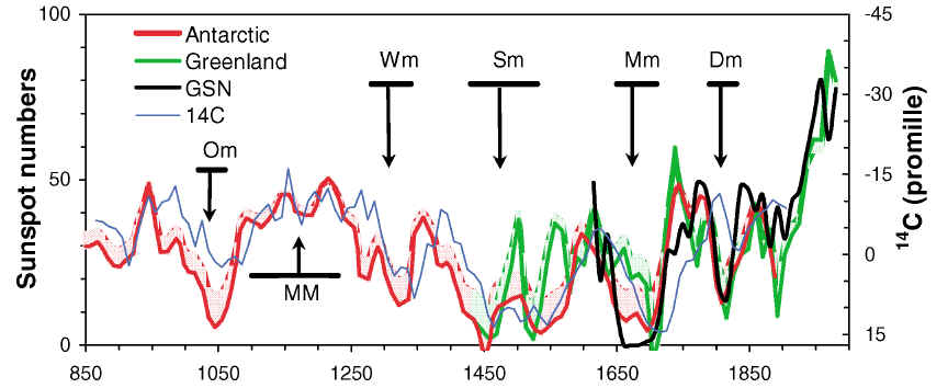
Usoskin et al PRL 2003 FIG. 2 (color). Time series of the sunspot number as reconstructed from 10Be concentrations in ice cores from Antarctica (red) and Greenland (green). The corresponding profiles are bounded by the actual reconstruction results (upper envelope to shaded areas) and by the reconstructed values corrected at low values of the SN (solid curves) by taking into account the residual level of solar activity in the limit of vanishing SN (see Fig. 1). The thick black curve shows the observed group sunspot number since 1610 and the thin blue curve gives the (scaled) 14C concentration in tree rings, corrected for the variation of the geomagnetic field [20]. The horizontal bars with attached arrows indicate the times of great minima and maxima [21]: Dalton minimum (Dm), Maunder minimum (Mm), Spo¨rer minimum (Sm), Wolf minimum (Wm), Oort minimum (Om), and medieval maximum (MM). The temporal lag of 14C with respect to the sunspot number is due to the long attenuation time for 14C [19].
The underlying Be-10 proxy series for Greenland (Beer et al 1990) is shown below as excerpted from Usoskin et al (Astr Astr 2004) (I have not been able to locate a digital version of the Dye 3 data.) The series are inverted in the solar reconstruction process. I discussed the Intcal data in an earlier post (url)
Usoskin et al 2004 Fig. 1. Raw and smoothed 10Be data. The lower curves (left axis) give the raw (thin curve) and the 1-2-1 filtered 8-year-averaged data from Antarctica (Bard et al. 1997). The upper curves (right axis) show the raw and the 11-year smoothed yearly data from Greenland (Beer et al. 1990).
Solanki et al (Nature 2004) had quite similar looking reconstructions – again the two Be-10 reconstructions and a àŽ”¬?C14, both fitted to reconstruct sunspot number.
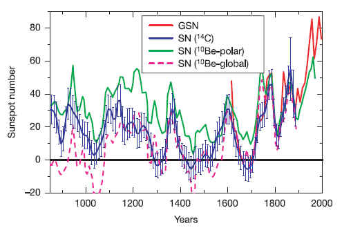
Solanki et al Nature 2004 Figure 2. Comparison between directly measured sunspot number (SN) and SN reconstructed from different cosmogenic isotopes. Plotted are SN reconstructed from D14C (blue), the 10-year averaged group sunspot number1 (GSN, red) since 1610 and the SN reconstruction14 from 10Be under the two extreme assumptions of local (green) and global (magenta, dashed) production, respectively. The slightly negative values of the reconstructed SN during the grand minima are an artefact; they are compatible with SN ¼ 0 within the uncertainty of these reconstructions as indicated by the error bars.
The C14-based solar reconstruction is archived at WDCP here, but not any of the other versions. Here is a plot of the archived data (matching the C14-based reconstruction above.) Sunspot data is digitally archived elsewhere. (This matches the purple series above ending ~1900 AD.)
Plot of archived data at WDCP matching C14 solar reconstruction of sunspot number.
In 2006, Usoskin et al GRL 2006 re-visited this reconstruction using a different geomagnetic series to normalize the data, obtaining similar results. (Jan 16, 2007) In response to a request yesterday, Dr Usoskin forwarded a digital version of the reconstruction in Usoskin et al GRL 2006, which is re-plotted below, showing both Holocene and millennium values. HE referred me to JàÆà⻲g Beer, the author of the Dye3 Be-10 series for that data, which I’ve requested. This series goes to 1995 on 10-year intervals, with recent values among the highest on record (the 2nd-most recent value is the highest in the entire series.)à’à As a potential contributor to the Holocene Optimum, this data version suggests a solar peak after the Holocene Optimum; it would be interesting to examine the basis of this reconstruction in detail at some point.
Usoskin et al GRL sunspot number reconstruction. Left – BP; right – detail denominated in years AD. The “record” is in 1985. Plotted from emailed data.
Muscheler Criticisms
Solanki et al (Nature 2004) was criticized by Muscheler et al 2005 in a Nature Brief Communications Arising, with Muscheler et al presenting a different reconstruction, also presented the version below in a post by Muscheler at realclimate: (See links to Muscheler articles)

Muscheler et al reconstruction (from realclimate) Figure 1: Reconstructions of the (11-year smoothed) solar magnetic modulation based on 14C data from tree rings combined with instrumental measurements (Muscheler et al.,2005). The purple curve shows the results according to a normalization using balloon-borne measurements. The black and green curves show results using an alternative normalization and the northern hemisphere (black) and globally averaged (green) 14C data. The red curve is the group sunspot number.
Muscheler stated:
As long as the differences between the 10Be records are not understood, conclusions based on only one of these records should be treated with caution. Atmospheric 14C concentrations, on the other hand, are much less sensitive to a climate influence during the last 1000 years and, therefore, can provide good estimates of the history of the sun. However, the disagreement between 14C-based solar activity and group sunspot number (Muscheler et al., 2005) should remind us that the variations of the solar activity are not yet completely understood.
Usoskin replied sharply to the Muscheler criticism arguing that they had improperly normalized their data:
We conclude that by basing their normalization procedure on inappropriate data, Muscheler et al. have heavily overestimated the solar modulation parameter before AD 1950, which was further exaggerated by the nonlinear relation between Qand .Unfortunately, when performing the normalizing procedure, they made use of an inappropriate data set, from which the long-term trend has been implicitly removed (see details in Solanki et al., 2005). This resulted in a distorted long-term trend in their reconstruction. When using the correct data set (called “alternative” by Muscheler et al., 2005), they obtained the results which are very similar to ours as the purple curve in Muscheler’s Fig.1 is close to our solar activity reconstruction from 14C (see Solanki et al., 2004). All other curves in Muscheler’s Figure are affected by this normalization flaw which is seen as a constant offset between the curves (all curves are parallel to each other before 1950). Actually, this large difference of about 300 MV between purple and green curves serves as their model uncertainties. Briefly, Muscheler, using a different (unpublished and unverified) method, obtained a result which differs from our results. We don’t think that just this difference provides a substantial basis to claim that our results are wrong.
Recent Discussions
Recent discussions by Bard QSR 2006 is online here and Muscheler et al QSR 2007 is online here. In addition to discussions covering the millennium, there are interesting issues regarding the Holocene, which I’ve not touched on here, but which recur in the references.
Update: New paper by MacCracken et al here
References:
Bard 2003 ftp://ftp.ncdc.noaa.gov/pub/data/paleo/climate_forcing/solar_variability/bard_irradiance.txt
Bard EPSL 2006 http://www.college-de-france.fr/media/evo_cli/UPL13816_Bard06EPSL.pdf
Beer, J., A. Blinov, and G. Bonani, et al., Use of 10Be in polar ice to trace the 11-year cycle of solar activity, Nature, 347, 164– 166, 1990.
J Beer, Long-term Solar Variability derived form Cosmogenic Radionuclides http://www.hao.ucar.edu/scostep/scostep11_lectures/Beer.pdf
MacCracken et al here
Muscheler et al Nature 2005 How Unusual is Today;s Solar Activity? http://www.cgd.ucar.edu/ccr/raimund/publications/Muscheler_et_al_Nature2005.pdf
Muscheler at realclimate http://www.realclimate.org/index.php?p=180
Musceler QSR 2007.Solar activity during the last 1000 yr inferred from radionuclide records http://www.climate.unibe.ch/~joos/OUTGOING/publications/muscheler06qsr_solar.pdf
Solanki et al Nature 2004 http://cc.oulu.fi/~usoskin/personal/nature02995.pdf NAture SI http://www.nature.com/nature/journal/v431/n7012/extref/nature02995-s1.pdf
Solanki et al Response to Muscheler http://cc.oulu.fi/~usoskin/personal/sola_nature05.pdf
Usoskin, I. G., Mursula, K., Solanki, S., Sch¨ussler, M., & Kovaltsov, G. A. 2002a, J. Geophys. Res., 107(A11), SSH 13-1 http://cc.oulu.fi/~usoskin/personal/2002ja009343.pdf from 1600 on.
Usoskin et al AA2003 http://cc.oulu.fi/~usoskin/personal/AG_2003.pdf
Usoskin, I. G., Solanki, S. K., Schu¨ssler, M., Mursula, K. & Alanko, K. A millenium scale sunspot number reconstruction: evidence for an unusually active Sun since the 1940s. Phys. Rev. Lett. 91, 211101 (2003). http://cc.oulu.fi/~usoskin/personal/Sola2-PRL_published.pdf
Usoskin, I. G.,Mursula, K., Solanki, S. K., Schu¨ssler,M. & Alanko, K. Reconstruction of solar activity for the last millenium using 10Be data. Astron. Astrophys. 413, 745–751 (2004). http://cc.oulu.fi/~usoskin/personal/aah4688.pdf
Usoskin, I.G., S.K. Solanki, M. Korte, 2006. Solar activity reconstructed over the last 7000 years: The influence of geomagnetic field changes, Geophys. Res. Lett., 33(8), L08103.à’à http://cc.oulu.fi/~usoskin/personal/2006GL0259211_pub.pdf


128 Comments
Steve M.,
I am pleased to see that you have started a thread on the role solar variability plays in climate change. I have a number of comments related to this area, especially with regard to the statements made by a number of climate modelers that the solar variability is not important to the change in temperatures seen in coupled climate models. In following comments, I will discuss thru a mathematical error analysis why this is the case based on references quoted in comments on my previous post.
To begin, I agree with Pat Frank that the physics in the coupled climate models is extremely crude (equations to follow), but I do not agree with him that numerical resolution is less important. To illustrate this point, I will refer to plots from a study of a number of models in my next comment. These plots (and some underlying mathematics) show conclusively that the models will not converge to the correct physical solution as the resolution is increased no matter how good the physics might be, that is, no amount of computing power will solve this underlying problem.
Then I would like to discuss the dominant role heating (parameterizations) have in the smaller scales of motion in the midlatitudes and for all scales of motion in the tropics. I will quote both theoretical and supportive practical references that illustrate these points. Thus, any errors in the parameterizations lead to immediate errors in the associated numerical model and that is one reason that numerical modelers are now using so called ensemble methods in an attempt to overcome these problems.
And finally I will discuss the possible impact the above arguments have on your feeling that solar variability is most likely to first have an impact near the equatorial region (ITCZ).
Tamino, I didn’t want to disturb your anonymity, just to have a name to call you. I sincerely hope you will find time in your work to continue this conversation.
A couple of comments on your excellent and most interesting post.
First, I agree that increasing CO2 will warm the world. The question is, how much?
It is generally accepted that without the greenhouse effect, the world would be about 33°C cooler. It is also generally accepted that the total downwelling “greenhouse” radiation is about 325 W/m2.
This indicates that the warming from greenhouse radiation is on the order of a tenth of a degree C per W/m2. This, as you know, is called the “climate sensitivity”. However, since parasitic losses increase with the greenhouse induced temperature rise (‘ˆ’€ T), it is likely that the current sensitivity is less than that. But let’s use that value.
It is also generally accepted that for a doubling of CO2, the forcing will increase by about 3.7 W/m2. Given a sensitivity of 0.1°C per W/m, this indicates that a doubling of CO2 will increase the average temperature of the planet by about 0.4°C.
This projected doubling of CO2 may or may not happen in the next century. If so, we may get as much as a 0.4°C warming. This, I must admit, doesn’t worry me. It warmed more than that last century, with no adverse effects.
Second, you seem to think that because the solar forcing correlates well with temperature until 1980 but diverges after that, this means that CO2 must be the cause of the post 1980 temperature rise. But to believe that, we’d have to assume that CO2 had no effect until 1980 (or it would have disturbed the solar correlation with the temperature), and then suddenly kicked into gear. Seems doubtful.
In fact, our understanding of climate forcing is very poor. Of 12 known forcings, the IPCC TAR rated our understanding of 9 of them as “Low” or “Very Low” … and that doesn’t include forcings that are not included in the TAR (biogenic aerosols, biogenic methane, plankton created aerosols, solar magnetism, cosmic rays, etc.) or unknown forcings. The fact that we cannot explain the post 1980 divergence proves nothing about CO2. We do not understand what causes the shifts in the PDO, or the timing of ENSO events, or why there were a lot of hurricanes in 2005 and relatively few in 2006, or why the AMO cycle is about forty years long … why do you think we should understand the recent warming?
Finally, you seem to think the burden of proof is on the skeptics, which is science set on its ear. We don’t understand the climate. You have a theory about it. Your theory is not yet advanced enough to make falsifiable predictions, so it is not yet possible for scientists to say anything definitive about the theory. In the absence of an ability to make falsifiable prediction, to support your theory you need evidence. Not absence of competing theories. Not computer models whose results vary by 800%. Evidence, that is to say, real world data. You say that there are a “vast number of evidences” for the theory that CO2 will cause large, significant warming. What is that evidence? For a start, how does your theory explain that 325 w/m2 of forcing only resulted in a 33° temperature rise?
My best wishes to you,
w.
Sorry, mis-posted to the wrong site … intended for another blog.
w.
Willis re #2 which blog? Might be interesting.
P
This blog … The guy seems quite nice, although very pro AGW.
w.
An early reference worth looking at is
Google Scholar currently lists 74 citations.
Here’s a “cold” Sun story from NASA:
link
NASA Solar Radiation and Climate Experiment Main page
here
more here: “We are all tremendously excited about what we will learn about the solar climate connection from SORCE,” said Bill Ochs, SORCE Project Manager at Goddard Space Flight Center. “We’re very proud of the mission team led by the University of Colorado and supported by Orbital Sciences Corporation. This mission is a great example of how NASA, universities, and industry can partner to create successful missions.” For more information about this mission to explore Earth’s climate please see: http://lasp.colorado.edu/sorce
SORCE meeting Oct. 2004:
“Decadal Variability in the Sun and Climate” link
It looks to me like in the Uroskin Fig 2, the Antarctia and C14 curves are offset 30-50 years (Antarctic peaks occuring before the corresponding C14 peaks). Is there a physical reason for such an offset?
Interesting presentation from the list provided by rocks
I’ve added in a plot of the newest Usoskin version from Usoskin et al 2006 from digital data emailed to me from Usoskin (who, not being a member of the Team, provided this information quickly.) I wonder how Crowley’s doing with his hard drive.
Hey- even the Team participated in that 2004 SORCE meeting:
link to presentation to spot the Hockey Stick. 😛
Thanks for the post on Solar effects, Steve. As you know I am very interested in this stuff. I’ll bet you won’t find the “pea under the thimble” syndrome with the Solar scientists. It looks like they are very willing to share their data and methodology.
#13. Actually, the record of archiving of solar series and reconstructions is rather poor. I’ve sent a request to Muscheler. We’ll see,
I too congratulate you on separating out this thread on extraordinary claims — this one solar.
re: 2 — fine post!
Steve M., as you probably know, according to Veizer, cosmic rays can also be used as a proxy for solar activity. His work has been criticized, but his rebuttal seems very convincing. Veizer also uses ice-rafted debris as a proxy.
Steve M.,
The solar variability is stated to be on the order of 0.1% over the period of a solar cycle of 11 years (see, for example, the article mentioned in this thread in comment 7 by welikerocks). For small relative variations in forcing, there is a mathematical (upper bound) estimate on the difference between solutions with a nominal forcing and with a nominal forcing plus a small perturbation. I will not bother you with these details unless someone claims that the estimate is not applicable. For such a small change in the forcing, it should be obvious that the relative errors in a coupled climate model would have to be less than 0.1% over the entire period of a solar cycle to ensure that the variation in solar forcing is not overwhelmed by the numerical, physical, and other errors in a coupled climate model. But according to a reference in a comment on my first post, climate models are unable to accurately predict the climate for a year, let alone 11 years. (I do not beleve the claim that a limited area climate model is more accurate than a global climate model because a limited area climate model must be forced at the lateral boundaries by unknown future boundary conditions.)
Is LaTex up on this site now so I can use equations if needed?
Steve M.,
In the presentation by the HT at the SORCE conference (see welikerocks #12), the team said that there is evidence that the solar cycle might play an important role in the climate. Isn’t that a major shift in their viewpoint? (Note that scientists at NCAR claimed no such important role for solar variability in a press release by Wigley et al.)
Gerald B.,
Solar variability over the last 300 years is thought to be near 0.3%. The usual 11 year solar cycle is 1/3 of that. We are interested in much more than just the contribution of the solar cycle right?
Interesting that large solar spots can dim the sun. Is it that the area covered by the faculae of a spot increases at rate much slower than that of the spot itself as a spot grows? I am not aware of any lengthy period of the sun being afflicted by large sun spots. Perhaps the Chinese or Greeks noticed such a thing?
We know that the Sun has cycles. We know that it has at least a very regular 11-year cycle (with significant variation among those cycles.)
We know that there is at least one longer-term cycle as well. The lack of sunspots in the early 1700s tell us that for sure. The other proxies show there is other variability, most indicating increases and decreases that are not as regular as the 11-year cycle.
The sunspot data shows us there is at least a 0.3% variation in the sun’s output. But sunspots are not the true measure of the sun’s total EM spectrum of output. The sunspots just tell us the Sun has cycles and is not the monolith-never changing object that the climate change community wants everyone to believe.
So the Sun has variability and cycles. The earth’s orbit and inclination also change resulting in a change in the amount of the sun’s energy impacting the climate.
With all these variations, why is there no model of the sun’s output energy? Why do no climate models incorporate a solar variation component? Why is the astrophysics community not contributing to this debate?
Solar output is not the only issue, and almost certainly not the main issue.
Changes in the sun’s magnetic field are also extremely important and have been implicated in playing a major role in cloud cover (because the sun’s magnetic field deflects incoming galactic cosmic rays, and GCRs seed clouds). Changes in solar magnetic flux are MUCH larger than the changes in EM output.
I am too lazy to look for a solid reference right now, but I think you will find the changes in solar magnetic flux are orders of magnitude greater than the changes in radiance, see WP
# 19 The expression “thought to be” is not precise.
I do not know the accuracy of these measurements, nor do I think anyone can state with absolute certainty the accuracy of these measurements
as there have only been satellite readings in the last few decades
and before that only qualitative guesses, e.g. the Maunder Minimum. What I am pointing out is that with variations in the forcing of any amount less than 1.0%, a coupled climate model will not accurately portray that variation given that there are larger relative erros in the numerics, physics, viscosity (cascade of entropy), etc.
#20 Good questions. Why not ask them.
#21 “Implicated” is not a precise mathematical term.
#22 here’s some more precise mathematics for your delectation:
Click to access sensitivity.pdf
Hello
as this is my first post here, I give you a short introduction of myself (hopefully not too boring, but nobody has to complain about beeing anonymus)
living in Switzerland, studied veterinary medecine, working in this profession, very interested in “climate change” to somehow get rid of all this fear you can get, when visiting alarmist sites (eg. RC)
I’m happy having found this site and especially somebody who did not buy the hockeystick and deconstructed it (the interview with Mann on BBC4 make me lose any faith in this person definitely)
[snip]
I can not judge on this at all, so I would be happy for your input
Gaudenz
Landscheidt’s work on Solar Inertial Motion and it’s possible relationship
to solar cycles was interesting (to me anyway). There are a few other
publications on SIM. His prediction for a soon to arrive Little Ice Age is
backed by some Russian Scientists, and others:
Nigel Weiss, professor emeritus of mathematical astrophysics in the University of Cambridge, discovered the process of “flux expulsion” by which a conducting fluid undergoing rotating motion acts to expel the magnetic flux from the region of motion, a process now known to occur in the photosphere of the sun and other stars. He is also distinguished for his work on the theory of convection, and for precise numerical experiments on the behaviour of complicated non-linear differential equations. Nigel Weiss is a recipient of a Royal Society Citation, he is a past President of the Royal Astronomical Society, and a past Chairman of Cambridge’s School of Physical Sciences. He was educated at Clare College, University of Cambridge.
RIA Novosti, 15 January 2007
http://en.rian.ru/russia/20070115/59078992.html
and NASA, perhaps:
http://science.nasa.gov/headlines/y2006/10may_longrange.htm
Below is an article that appeared today in the Financial Post. I agree with Weiss.
Will the sun cool us?
LAWRENCE SOLOMON
Financial Post
Friday, January 12, 2007
The science is settled” on climate change, say most scientists in the field. They believe that man-made emissions of greenhouse gases are heating the globe to dangerous levels and that, in the coming decades, steadily increasing temperatures will melt the polar ice caps and flood the world’s low-lying coastal areas.
Don’t tell that to Nigel Weiss, Professor Emeritus at the Department of Applied Mathematics and Theoretical Physics at the University of Cambridge, past President of the Royal Astronomical Society, and a scientist as honoured as they come. The science is anything but settled, he observes, except for one virtual certainty: The world is about to enter a cooling period.
Dr. Weiss believes that man-made greenhouse gases have recently had a role in warming the earth, although the extent of that role, he says, cannot yet be known. What is known, however, is that throughout earth’s history climate change has been driven by factors other than man: “Variable behaviour of the sun is an obvious explanation,” says Dr. Weiss, “and there is increasing evidence that Earth’s climate responds to changing patterns of solar magnetic activity.”
The sun’s most obvious magnetic features are sunspots, formed as magnetic fields rip through the sun’s surface. A magnetically active sun boosts the number of sunspots, indicating that vast amounts of energy are being released from deep within.
Typically, sunspots flare up and settle down in cycles of about 11 years. In the last 50 years, we haven’t been living in typical times: “If you look back into the sun’s past, you find that we live in a period of abnormally high solar activity,” Dr. Weiss states.
These hyperactive periods do not last long, “perhaps 50 to 100 years, then you get a crash,” says Dr. Weiss. ‘It’s a boom-bust system, and I would expect a crash soon.”
In addition to the 11-year cycle, sunspots almost entirely “crash,” or die out, every 200 years or so as solar activity diminishes. When the crash occurs, the Earth can cool dramatically. Dr. Weiss knows because these phenomenon, known as “Grand minima,” have recurred over the past 10,000 years, if not longer.
“The deeper the crash, the longer it will last,” Dr. Weiss explains. In the 17th century, sunspots almost completely disappeared for 70 years. That was the coldest interval of the Little Ice Age, when New York Harbour froze, allowing walkers to journey from Manhattan to Staten Island, and when Viking colonies abandoned Greenland, a once verdant land that became tundra. Also in the Little Ice Age, Finland lost one-third of its population, Iceland half.
The previous cooling period lasted 150 years while a minor crash at the beginning of the 19th century was accompanied by a cooling period that lasted only 30 years.
In contrast, when the sun is very active, such as the period we’re now in, the Earth can warm dramatically. This was the case during the Medieval Warm Period, when the Vikings first colonized Greenland and when Britain was wine-growing country.
No one knows precisely when a crash will occur but some expect it soon, because the sun’s polar field is now at its weakest since measurements began in the early 1950s. Some predict the crash within five years, and many speculate about its effect on global warming. A mild crash could be beneficial, in giving us Earthlings the decades needed to reverse our greenhouse gas producing ways. Others speculate that the recent global warming may be a blessing in disguise, big-time, by moderating the negative consequences of what might otherwise be a deep chill following a deep crash. During the Little Ice Age, scientists estimate, global temperatures on average may have dropped by less than 1 degree Celsius, showing the potential consequences of even an apparently small decline.
Dr. Weiss prefers not to speculate. He sees the coming crash as an opportunity to obtain the knowledge necessary to make informed decisions on climate change, and the extent to which man-made emissions have been a factor.
“Having a crash would certainly allow us to pin down the sun’s true level of influence on the Earth’s climate,” concludes Dr. Weiss. Then we will be able to act on fact, rather than from fear.
Lawrence Solomon is executive director of Urban Renaissance Institute and Consumer Policy Institute, divisions of Energy Probe Research Foundation.
CV OF A DENIER:
Nigel Weiss, professor emeritus of mathematical astrophysics in the University of Cambridge, discovered the process of “flux expulsion” by which a conducting fluid undergoing rotating motion acts to expel the magnetic flux from the region of motion, a process now known to occur in the photosphere of the sun and other stars. He is also distinguished for his work on the theory of convection, and for precise numerical experiments on the behaviour of complicated non-linear differential equations. Nigel Weiss is a recipient of a Royal Society Citation, he is a past President of the Royal Astronomical Society, and a past Chairman of Cambridge’s School of Physical Sciences. He was educated at Clare College, University of Cambridge.
This may be a duplicate post…
Here is an interesting dichotomy.
On one hand you have anthropomorphically derived incremental (small) greenhouse gases that are thought in isolation to have a minimal impact upon global temperatures but induce feedbacks that will ramp temperatures to an extent that will endanger the biosphere.
On the other hand you have apparently small changes in solar forcing that are thought to have a minimal impact upon global temperatures and induce no feedbacks and therefore do not endanger the biosphere.
What is the difference between the two? Might I suggest the “a” word?
#27-You really didn’t say anything, did you? Al Gore has said as much, ad nauseum.
Solar variability caused the Little Ice Age, and likely contributed to the Medieval Warming Period. The ancients worshipped their sun gods for a very good reason.
😉
S. M. Tobias & N. O. Weiss, Resonant Interactions between Solar Activity and Climate, Journal of Climate, Volume 13, Issue 21(November 2000)
An interesting theory.He has some numbers different from what I gave in #19 and support for them.
This new blogger is confused about how to post a chart. Could someone give me a hand? Should the image show in the Preview section prior to hitting submit comment, or do you just enter the url and hope for the best? Thanks.
Click Img in the quicktags above the comment insert box and insert the url of the image.
I was impressed when I first saw this figure a few years ago.
How good is the relationship depicted which, at least to a layman, seems to demonstrate rather convincingly that global temperatures correlate well with variations in solar activity (maybe even better than with CO2)?
re 32:
Click to access DamonLaut2004.pdf
re 33: http://www.marshall.org/article.php?id=15
BTW, jae, the article that the marshal institute piece is referring to, is by Lassen and Thejll, the very same people who are reporting the correlation between solar cycle length and temperature that you place so much store by. They report that with additional data, the correlation collapses in recent decades. They also report (and Soon fails to mention in his Marshall Institute hit piece) that they examined the possible impact of mistakes in their assumptions about future cycle lengths, and that the chance of them being short enough to seriously affect their conclusions about the collapse of the correlation is small.
IOW, the people who report the correlation are ALSO the people who now say it appears to be a factor in climate, but is not a dominant factor in the recent temperature increases.
Lee: I don’t understand your post. The relationship cannot be proven one way or another without two more solar cycles, as I understand it.
This is a link to a paper written in 1987. They make some predictions on things to come. I don’t think that we are going to have to wait very many years to find out whether or not they were right.
A objective overview of ‘CO2 or Solar’ from Nir Shaviv here, plus a demolition of the ‘straw man’ argument used against the solar-cosmic rays-climate connection by the likes of RC, in comments at the end:
http://www.sciencebits.com/CO2orSolar
I got the Barycenter dates from this 1987 article and sketched out this chart. What do you think the chances are of going into another minimum in the next 15 years?
[img]http://www.bnhclub.org/JimP/Pictures/colddate.JPG[/img]
Well, that didn’t work.
Doesn’t it strike you that these solar proxies have a much better fit to historic temperature changes than anything milked out of tree rings?
The Dalton minimum showing up hits home for me. I have an old wood clock built by Chauncey Jerome around 1820. He describes almost freezing to death in the summer while on the road. It was some time after the war of 1812 in the Dalton minimum. I hope we don’t have that sort of weather in my lifetime.
Here is a very interesting article that I found that comes to the conclusion that the sun is more active now than it was even during the MWP. Very interesting read.
http://prola.aps.org/pdf/PRL/v91/i21/e211101
#42
cbone, can you give us more details. The link wants my password. I do not have one. How about a summary of the main points.
Re: #42, 43
Its from Physical Review Letters v91 issue 21, you can buy the full article here.
Most active sun in the last 1000 years. Now where have I heard something else like that?
I ran across possibly one more piece of evidence from Woods Hole oceanographers suggesting we are going into an extended cooling period. Are past minimums preceded by high solar activity? Is it the shut down of the thermohaline circulation the event that sets off these minimums?
#45. Interesting article from 2002. I was amused by the adverb added to the following quote from Keigwin:
Sorry about the link. It worked fine last night, now it wants a password. Odd.
Basically the article was a reconstruction of solar activity and came to the conclusion that the recent solar activity is greater than even during the MWP.
Here is another article, that hopefully won’t disappear.
Solar activity, cosmic rays, and Earth’s temperature: A millennium-scale comparison
Click to access 2004ja010964.pdf
Several items of interest in this one. First, guess who shows up in the temperature comparisons? Why the good ol’ hockey stick! Figure 2 is also rather interesting, it is a reconstruction of sunspot numbers. The coorelation information, I admit, is beyond me to analyze. Anyone care to take a stab at it?
#44 Check this out. According to NOAA Paleoclimatology Program there are not any sunspot years in the last 2000 years and longer that even come close to the last 60 years.
#46 What I found interesting about this article is that these researchers would all of a sudden go against popular opinion and start sounding the alarm about global cooling. They must have some pretty convincing data. It would be interesting to see if the slow downs in the thermohaline circulation coincided with the Minimums and whether or not there really is as much fresh water in the North Atlantic as what they indicate.
Paul Biggs (#23),
I have obtained a copy of the article and on a brief perusal the author clearly has stated a number of caveats in his analysis. After I have finished the tutorial I refer to in #1, I will be happy to read the article in detail and present a discussion of the assumptions and results.
So for what it’s worth; I noticed a sharp dip in sunspots around 4800 BP. This corresponds to this Asteroid Impact event. So maybe cloud cover affects the sunspot data? This graph shows how the major volcanic eruptions line up with recent minimums and sunspot data. I don’t have any data on major volcanic eruptions going back any farther. Are there any data sets available that just track SO2?”¢’¬?Assuming SO2 corresponds to volcanic eruptions.
Has anyone tracked current sunspots using 1600’s technology and methods?
JP (#51),
In the 1987 manuscript you mentioned, I believe Tom Wigley (NCAR) is mentioned as a revewer.
Re;50 Gerald – I’m interested in seeing your analysis. There have to be caveats due to the uncertainties in a not fully understood, complex climate system.
What do you think of this image overlaying the Mann and Moberg temp reconstructions over the Usoskin sunspot number reconstruction?
There are two set of curves, one comparing the Mann hockey stick to curves showing sunspot activity. The other compares the Moberg 2005 curve to the same sunspot curves.
Here’s what I find interesting:
– The Moberg curve (blue curve) follows the Antarctic curve (red) pretty closely, but it tracks almost exactly the same shape as the Greenland curve (green) when it sweeps up in a steep curve in the 20th century.
– The hockey stick curve (orange curve) doesn’t do as good a job of tracking with the sunspot curves, in fact it looks like it averaged out the highs and lows (read “MWP” and “LIA”) to come up with a relatively smooth shape, but even so, it’s still a fair match to the sunspots, especially when it sweeps upward in the 20th cent.
The Antarctic and Greenland curves came from the image from Usoskin’s millennium-scale sunspot number reconstruction that Steve also provided above.
(If the image I gave is too small to see clearly, there’s a much larger version here.
I linked to the wrong version of the comparisons, Willis had recommended that I add the y-axis and I did it in this graphic:
http://farm1.static.flickr.com/132/371632655_6037f3dee0.jpg?v=0
The left side is measuring sunspot numbers, the right side, temperature anomaly values
To see the larger version go to http://www.flickr.com/photo_zoom.gne?id=371632655&size=l
Steve, I’m curious why you don’t show any graphs comparing these plots to sunspot number. I have read that sunspot number is considered a good solar proxy although I don’t think the phase always matches up.
Chris, jae and everyone,
There’s a chart that plots tree ring data and solar on this page (but it stops too short) : “An experiment onboard shuttle mission STS-107 is monitoring the Sun’s variable brightness. Scientists say it’s crucial data for understanding climate change.” here (sorry if this has been shared already) And another link for the AGU is found for “Solar Variability and Climate Change” here Seems to matter to some people!
JP this is a volcanic eruption that I have never heard of that happened in 1912:Novarupta Wonder how many we dont not about at all?
Sorry. “not” should be “know” in #57
John Creighton (#56):
If the sun were in a consistent warming or cooling period, I believe that there would be a lag because of the mathematical (integral) effect of changes in the external forcing. As mentioned by others, this is not straight forward, especially over a short time period, because of clouds and other complicated interactions. But the plots of the relationship between sunspot numbers and temperature are exactly what I had hoped that someone was willing to take the time to do because that represents an analysis not based on coupled climate climate models that have large errors as indicated in my first comment on this thread. Thank you Chris. The plots are most illuminating, especially given all of the questionable claims by the IPCC. If these results hold up, I also believe they can be used to support Steve’s ideas about the ITCZ.
Re #57 welikerocks,
Every time I read a number for solar intensity variation over the last few hundred years it is different. That 2003 NASA article says it was thought to be 0.6% less bright in the LIA. I don’t think we really know. Wonder who NASA got this from.
John G. Bell, I don’t know? I noticed too, that the websites and studies that you get when you google the sun+climate, start out full of information then they seem to just stop. By that I mean they haven’t been updated in a couple of years, or you can’t find anything current- except for the discription of the project or research, the charts are old and there isn’t anything “new” to read. (Hope that makes sense-I dont want to be “unscientific” and say they all are like that-I know there might be research in other countries I can’t read because I can only read English, etc)
FYI, the sunspot number curves comparison with the global temp curves has been updated to include the Usoskin GRL sunspot number reconstruction that Steve provided above:
To see the larger version click here
Chris (#62):
The consistency between the two ice cores and Usoskin’s reconstruction seems to me to be rather striking, especially when they are more in line with the LIA and MWP. Congratulations! Now that you have these plots, it might be useful to have a plot that starts at the same time as the Antartic ice core so that one can see the sunspot curves on the rhs in more detail? I am quite curious to see what Steve M. says about these curves and proxies and, to clarify the state of solar science, if maksimovich agrees with my responses to his answers.
Because I cannot use LaTeX yet, I am preparing a nonmathematical presentation for a general audience as promised in #1.
IPCC SPM WGI 4AR (page 3):
(emphasis HE)
Hans (#64),
Don’t you just love the qualifying phrase “estimated to cause”. By whom and how?
Where are the details?
Wait until May. Then no journalist will be interested anymore.
“Don’t spoil a good story by digging up conflicting details”,
which is a paraphrased translation of Francisco van Jole’s:
“Een mooi verhaal moet je niet kapot checken”
Re 64,65,66
They used the following methodology. A composite series for the time scale from;
a) Solanki and Krivova (2003, SK) which uses
(i) solar cycle amplitude for secular variation with
(ii) a 2 Wm-2 increase since the Maunder Minimum and
(iii) the FràÆàlich and Lean reconstruction for the satellite era.
Our reasons for choosing cycle amplitude are as follows. Very little justification is given for using cycle length except that (a) it fits well with the global average temperature record before 1970 and (b) shorter cycles are more intense because there is not time for a previous cycle to decay before the subsequent one starts. We reject reason (a) on the basis that it is important to seek reconstruction methods independent of the climate system. (b) suggests that cycle length is only an indirect measure of cycle amplitude. Furthermore, the value of cycle length is more difficult to determine, as is evidenced by the differences between the time series of cycle length produced by Friis-Christensen and Lassen (1991), Fligge et al (1999) and Lockwood (2001). For this pragmatic reason, and until a physical basis is established for the use of cycle length, we reject it in favour of the direct use of amplitude.
SK discuss the possible values for the long-term increase in TSI since the Maunder Minimum (MM). They present an overview of current results and opinions concerning possible values, including estimates based on UV spectral lines, open magnetic flux and magnetograms and conclude that it probably lies in the range 2-4 W m-2. We recommend the value at the low end of the range.
The results of FràÆàlich & Lean (1998, updated to present on http://www.pmodwrc.ch) show essentially no difference in TSI values between the cycle minima occurring in 1986 and 1996.
The results of Willson & Mordinov (2003), however, show an increase in irradiance of 0.045% between these dates. The discrepancy hinges on assumptions made concerning the degradations of the Nimbus7/ERB and ERBS/ERBE instruments, data from which fills the interval, July 1989 to October 1991, between observations made by the ACRIM I and II instruments. If such a trend were maintained physically, it would imply an increase in radiative forcing of about 0.1 Wm-2 per decade. Compared in terms of climate forcing, this is appreciable, being about one-third that due to the increase in greenhouse gases averaged over the past 50 years.These discrepancies are important because all the available TSI reconstructions discussed below either use directly, or are scaled to fit, the recent satellite measurements, using one or other of the TSI composites.
Similar observations for instruments onboard Soviet-Russian satellites is documentated.
Let us now identify differences in the physics of Solanki/Lean.
1) Whilst each is using datasets of differing phenomena e.g. sunspots, faculae, prominence etc. to model TSI each group has opposite views on changes in the magnetic flux and heliospherical modulation..
Indeed, the idealised modelling work of Lean et al (2002) suggests that TSI depends on the solar total magnetic field, of which only a small proportion is the open flux.These authors argue that, although there has been an upward trend in open flux, the total flux returns essentially to zero at each solar minimum giving no long-term trend in solar irradiance. This work is controversial; other authors (e.g. Solanki et al, 2002) are of the opinion that open flux is related to total flux so that either may be used as a proxy for irradiance and that the overlap (in time) of consecutive solar cycles causes the total flux not to return to zero at solar minimum.
This is indeed an ideological contrast, they cannot be both correct.
Here we deal with 2 comparative phenomena,
i) The stellar magnetic field
ii) The helioshperic interplanetary magnetic field.
First is the Stellar magnetic field a surface phenomena NO!
Magnetic fields and electrical currents are above the surface and present in the solar atmosphere.
Second why is the Stellar magnetic field variable? Rotation, internal convection ,finite B
The heliophysical (not solar) origins of the interplanetary magnetic field.The heliophysical currents are underestimated and not fully appreciated by many researchers.
Heliophysical current sheets are the main contributor to the field.
An interesting statement from L.Grey et al in the review of the solar understanding for the IPCC for AR4 is
“⠠ Uncertainties in the reconstruction of historical TSI mean that the value of solar radiative forcing from 1750 to the present is even less well established than was perceived for the IPCC (2001) TAR but, based on the current consensus that the secular trend in TSI is smaller than previously assumed, it may be appropriate for the value to be reduced from the TAR value of 0.30 Wm-2 to about 0.28 Wm-2.
Of course if we view the measurement problem ,some questions on assumptions for the summary for policy makers arise in the simple expression sensitive to initial conditions .
“⠠ Comparison of measurements from different satellite observing systems shows that the present day value of total solar irradiance is only known to approximately 0.15% (~2 W m-2). Its variation over the past two solar cycles is known, with greater accuracy, to be ~0.08% (~1.1 Wm-2) but difficulties encountered in the intercalibration of the instruments mean that the existence of any underlying trend in TSI over the past two solar cycles is uncertain.
“⠠ Most reconstructions of past values of TSI rely on
(i) empirically-derived relationships between proxy indices of solar activity and measurements of TSI and
(ii) assumptions concerning long-term secular changes in the à’”¬Åquiet Sunà’”¬?.
The former are fairly well established and, to a certain extent, can be reproduced by physical models. The latter are not well known and continue to be highly controversial.
Gerard I will address the questions that arose in the IPCC thread. Indeed the statement that the observed phenomena is too complicated and theories oversimplified, as a rule that make an accurate solar models possible or realistic is a paradox,that I agree with somewhat, but creates the logical conundrum for non-circular answers.
#64. The reduced solar estimate is from Wang et al 2005, which is cited in the Second Order Draft chapter 2. An irony here is that, if this estimate is correct, the various studies purporting to reconstruct millennium climate have all used solar variations which are too large, implying either that the efficacy of solar variations is much larger than previously thought or that past changes are even more unexplained.
Steve M.,
Recall that coupled climate models use a viscosity that is much larger than that of the real atmosphere (see my initial post under modeling). Because a coupled climate model is not like the real atmosphere, the physical forcings (parameterizations) are necessarily unrealistic (this can be shown using two very simple mathematical equations when LaTex becomes available). I would surmise that these model forcings, e.g. solar, must be larger than the real forcings because the coupled climate models have a much faster removal of energy and enstrophy than the real atmosphere.
I will pose a question that will appear at the beginning of my new presentation.
If a physical system has an exponentially growing solution, what happens to the continuous solution if the wrong initial value is chosen or to any numerical approximation of the continuous solution?
Gerald, I couldn’t find your post on viscosity “under modeling”. Could you post a link?
Thanks,
w.
Willis (#70):
See the post “Gerry Browning: Numerical Climate Models” on May 15 under modeling. (Actually it should be Jerry or Gerald 🙂
I will be happy to answer any questions you have about any of my posts in nontechnical text or mathematical equations (once LaTex becomes available).
Jerry
Gerald, thank you kindly for the reference. I am currently attempting to understand your post completely. It is fascinating.
Much appreciated,
w.
Willis (#72):
AFter reading the post on Numerical Climate Models, you might want to peruse the manuscript
Comparison of Numerical Methods for the Calculation of Two-Dimensional Turbulence
G. L. Browning and H.-O. Kreiss
Mathematics of Computation
Volume 52, No 186 (April 1989), pp. 369-388
Igmore the mathematics and just read the text and look at the contour plots.The plots make very clear what happens if insufficient resolution is used for a given kinematic viscosity for the incompressible NS equations and how the minimal scale estimate provides accurate information as to the amount of resolution needed to correctly resolve the solution for a given kinematic viscosity. The minimal scale estimate and examples make it very clear why low resolution Coupled Climate Models necessarily use viscosities that are orders of magnitude too large. Hence, necessarily, the forcings are nonphysical.
re: #73
So what does this mean practically? Does it slow down error propagation down to the point where steady results can be obtained? If so, how do the results compare to a case where an artifically “easy” normal viscositiy case could be calculated (if that’s possible).
Thanks to lubos the following review link:
Click to access scherer-etal-2007SSR.pdf
Interstellar-Terrestrial Relations: Variable Cosmic Environments, The Dynamic Heliosphere, And Their
Imprints On Terrestrial Archives And Climate
K. Scherer, H. Fichtner, T. Borrmann, J. Beer, L. Desorgher,E. Flükiger, H.-J. Fahr, S. E. S. Ferreira, U. W. Langner, M. S. Potgieter, B. Heber, J. Masarik, N. J. Shaviv And J. Veizer
Space Science Reviews (2006)
DOI: 10.1007/s11214-006-9126-6
#73 — Gerald, on page 386 of your paper, where you discuss the results in Figure 8, of tuning a hyperviscosity calculation to have zero amplitude coincident with regular viscosity, you say that, “the general features of the soution are similar [but] the details are quite different. … It is possible to have either the blob amplitide or spatial extent similar, but not both.”
Is that analogous to the reason why, e.g., climate models can be tuned to get the cloudiness right, or the precipitation, but not both?
Pat Frank (#76):
The turbulence results are for the unforced (spin down) case. The reason for doing the study that way is that once forcing is included, one can obtain any solution (spectrum) that one wishes. (This can be shown thru a simple mathematical argument that I will be happy to include if you want now that John A has LaTeX up again.) The main point to be made is that a different spatial spectrum is obtained depending on the size and type of viscosity included in a numerical model. (Higher order forms of viscosity eventually lead to spectrum chopping.)
The forcings in Coupled Climate Models (and weather models) have spatial and temporal mathematical discontinuities. This causes the numerical solution to be very rough (discontinuous). (There is a published manuscript by Heinz and me on this issue that I can provide if you are interested.) In order to make the numerical solution appear smooth, the viscosity in these models must be orders of magnitude too large, or the models will blow up. The smoothing can be either explicit (large viscosity coefficient) or implicit (chopping the spectrum or included in the numerical method). Certainly, if the viscosity coefficient is sufficiently large, a steady state will be reached very quickly because the system behaves more like a heat equation than a hyperbolic system with small dissipation.
The current claim is that more resolution (computing power) will help. But that is not the case. I currently am working on that presentation.
Let me know if I have adequately answered your questions or if you would like me to clarify any of my responses.
Jerry
Dave Dardinger (#74):
Hopefully some of your questions have been answered in my response to Pat Frank. One of the problems with using the incorrect viscosity is that the cascade of enstrophy is incorrect. As the resolution is increased, the cascade process improves, but then other problems will appear as will be discussed in my forthcoming presentation.
I attended a seminar by one of the lead authors of WG1 and specifically asked him about the accuracy of the atmosphere ocean interface in their coupled climate model. He did not have a clue about that interface, i.e. the model is being used as a black box.
Re 77:
Will this numerical stabilization process have the unintended consequence of suppressing regional and global scale unforced oscillations in climate?
Wow Hans (and Lubos)…that paper is pretty impressive. It seems one of their primary unknowns was the conclusive GCR/cloud link. Are either of you aware of whether they have any plans to update their research and modeling to reflect the 2006 Svensmark finding from the SKY experiment? It seems that including those findings would greatly strengthen their GCR/Cloud section.
Re: 77 and 78
Interesting – I’m not as familiar with the guts of our climate model, CCSM, as I should be, but if it has unrealistically large viscosity, I’d be surprised. Also, can you give us the name of the WG1 lead author whose seminar you attended?
Douglas Hoyt (#79):
I believe all current climate models use the hydrostatic approximation for the atmospheric portion (although some are considering moving to a nonhydrostatic system). The hydrostatic system is extremely sensitive to errors, especially as the mesh is refined. (References available, but you might want to wait until Monday when much of my presentation will be ready.) More serious is the fact that because the models do not resolve many physical phenomena (fronts, hurricanes, tornadoes, etc.), the forcings (parameterizations) are very crude approximation of reality tuned to make a model appear realistic. These approximations affect the weather forecast models in a manner of hours (only saved by updating the models with new observations of the jet stream every few hours – see my post on numerical climate models) and become even more crucial near the equator and for smaller scales of motion in the midlatitudes. As has been discussed on several threads, the dynamical equations change character as one moves upwards in the atmosphere (e.g. plasma equations are more appropriate in the ionosphere), but coupled climate models do not change the equations.
Gary Strand (#81):
What are the horizontal number of grid points in latitude, longitude, and the vertical direction. How many points are removed during the dealiasing (chopping) process and what other forms of dissipative or smoothing operators are there in the atmospheric and oceanic portions (including numerical dissipation). Are there any switches in the parameterizations? What is the accuracy of the atmospheric/oceanic interface and how is that interface parameterized. What happens to features that develop in the smaller scales of motion as the enstrophy rapidly cascades down the spectrum? Are the smaller scale features important to the energy balance and how accurately is the inverse cascade determined? Are the hydrostatic equations appropriate for smaller scales of motion?
Gary, I hope that you reply to Gerry Browning’s questions.
Mr. Strand! We are waiting!
Re: 85
Patience. I don’t operate on a schedule convenient for you.
Re: 83
The resolution isn’t fixed – it can be chosen by the user. Paleoclimate runs typically use T31 for the atm and land surface, and roughly 3 degrees for the ocean and sea ice. For the IPCC AR4 runs, we used T85L26 atm and land (10 levels), and a displaced-pole 320x384x40 (about 1 degree in x and y) ocean, the same horizontal resolution for sea ice. The T85 represents the triangular truncation at 85 wave numbers.
The flux coupler interpolates (conservatively) between the atm/lnd and ocn/ice.
“Are there any switches in the parameterizations?”
What you mean isn’t quite clear to me.
Your other questions can be answered more thoroughly and accurately via the CCSM documentation. They’re quite complicated – along the lines of “how does it work”, which isn’t answered briefly.
Gary, you say:
Not being a climate modeler, I’m not familiar with CCSM documentation. Picking one of Gerry’s questions at random,
could I trouble you for a page reference within the documentation that deals with this issue.
Gary Strand (#87):
Instead of stating that the resolution can be chosen by the user (which is the case for any reasonable numerical model) and then stating that it is triangular truncation T31 or T85 (doesn’t mean much to people not familiar with the pseudo-spectral method), please state how many grid points that translates to in longitude so that people can tell what physical features can be resolved in the atmosphere. Also please state how many waves are thrown away in the dealiasing process in the corresponding FFT.
I looked briefly at the documentation of CAM3 and I thought the site said it was not finished because of inadequate manpower at NCAR?
In the documentation I could find, there are clearly dissipation terms on both the divergence and vorticity equations (in addition to any dealiasing, time filters, etc.). What are the types of these dissipation terms and what are the coefficients?
One degree resolution (~ 100 km ) for the ocean model means that the mesoscale eddies in the ocean are not properly resolved and neither are the boundary layers, e.g. the Gulf Stream. I believe these features are crucial to the climate? What equations are used in the ocean model, what type of numerical method, and what type of dissipation?
The flux coupler interpolates conservatively, but that does not describe the accuracy of the coupler or if that is a reasonable physical process.
Do any of the parameterizations have Fortran “if tests” or the equivalent (especailly the cloud parameterizations).
At what altitude is the top of the model and what boundary condition is used there?
Re #88
The section of CCSM documentation that deals with that general issue does not appear (based on a one-hour scan) to deal with that specific question. In other words, the high-level documentation appears to be inadequate to answer such a low-level question. In which case it would be desirable to have access to the code itself. However CCSM’s policy on code release seems clear:
“Attention, all planets of the Solar Federation …”
GISS model code is online … I wonder why the NCAR doesn’t do the same.
w.
Willis,
I have decided to write a brief text only presentation (with appropriate references) by Monday in order to avoid the LaTex interface problem and to ensure that it will be readable for a general audience. Then
if someone wants additional details, they can look up the references
or I can write some mathematical equations using the tex tag labels
to answer individual questions. That should be the easiest and quickest way to make the points. I will send the text presentation to Steve M. for posting as I did before.
BTW, the answer to the question is that the hydrostatic equations are not appropriate for smaller scales of motion as will be seen in the presentation.
Jerry
Re: 91
The primary NCAR model, CCSM, is available for download. Only a verified registration is required.
#93. Gary, could you give me a page reference for my question in #88.
Jerry B, sounds good. I look forward to it.
Regarding the CCSM model resolution, their FAQ states:
Ooooh, a little touchy about “vertical levels”, are we? … In any case, that’s the story for CCSM2. There is also the newer version, CCSM3, but its results are less lifelike than CCSM2 … go figure. Since this is a “coupled” model, with separate ice, atmosphere, land, and ocean models, this brings up an interesting question ‘€” how does one calculate the required resolution for a given viscosity when going from model to model, and how is that calculation affected by the fact that the atmosphere and land models have a different resolution from the ice and ocean models … Jerry, I leave that question for you, as I haven’t a clue …
w.
Re: 95
CCSM3 simulations for the AR4 were run at T85L26 and gx1v5 resolution – 4x the resolution of T42 in the horizontal directions. The “v5” for the ocean and ice indicates a minor revision of the grid. The ocean grid was designed to have increased resolution over the equator and the North Atlantic – to assist in resolving eddies and other features.
But thanks for looking up that information and posting it here. Saves me some time.
Willis,
How do you know that the results are less lifelike in CCSM3 than in CCSM2?
Note that the triangular truncation number indicates the number of waves retained, not half the number of grid points in longitude, e.g. T42 has 128 grid points in longitude which means there should be 64 waves in the FFT, but only 42 of them are kept in the triangular truncation. Isn’t this equivalent to chopping the spectrum at every iteration (also referred to as dealiasing)? Chopping is a limit of higher order dissipations (see turbulence manuscript). Also note that it effectively reduces the resolution.
I bet the dissipation coefficients in the atmospheric model are tuned to prevent spectral blocking. All one has to do is look at the coefficient values for different resolutions.
Willis,
The new post is ready. Short and sweet, but hopefully easy to understand for everyone and very illuminating.
I have sent a copy to Steve M. for posting and have made a suggestion that he start a new thread, but that, of course, is up to him.
Jerry
Jerry, I fear my memory betrayed me, and I was thinking of the Princeton CM2.1 and 2.0 models. A couple of years ago, I took a look at the model hindcasts used in the Santer et al. paper about tropical tropospheric temperatures, “Amplification of Surface Temperature Trends and Variability in the Tropical Atmosphere.” Here are some results:
Figure 1. Surface Temperature Observational Data and Model Hindcasts. Colored boxes show the range from the first (lower) quartile to the third (upper) quartile. NOAA and HadCRUT (red and orange) are observational data, the rest are model hindcasts. Notches show 95% confidence interval for the median. “Whiskers” (dotted lines going up and down from colored boxes) show the range of data out to the size of the Inter Quartile Range (IQR, shown by box height). Circles show “outliers”, points which are further from the quartile than the size of the IQR (length of the whiskers). Gray rectangles at top and bottom of colored boxes show 95% confidence intervals for quartiles. Hatched horizontal strips show 95% confidence intervals for quartiles and median of HadCRUT observational data.
As you can see, the two CM models were the worst of all of the models, with 2.1 worse than 2.0. However, the CCSM3 model results were also well out of the 95% confidence intervals … but then that was true of the majority of the models. The results for first and second differences were also similarly bad, none of the models were within the 95% confidence intervals by all three measures. Despite this, of course, they were all used and were all weighted equally … I’ve never understood that about climate modelers. In any other field, people want to show that their model is better/faster/slicker/more accurate than the next guy’s model, if only for bragging rights … but these guys seem to be in some kind of agreement that if your model a) has lots of code, and b) employs lots of people, that it’s good enough for the IPCC … go figure.
Note that the figure above is measuring only the simplest statistics of the surface temperature, the mean and distribution, and most of the models can’t even get that right … but we’re supposed to trust them for trends, and feedbacks, and all the rest … and this is for the tropical ocean temperature, which changes slowly and is spatially much more consistent than the land. I shudder to think what the corresponding graph for the land temperatures would be like …
w.
Well, let me try that again. Here’s the graph:
Figure 1. Surface Temperature Observational Data and Model Hindcasts. Colored boxes show the range from the first (lower) quartile to the third (upper) quartile. NOAA and HadCRUT (red and orange) are observational data, the rest are model hindcasts. Notches show 95% confidence interval for the median. “Whiskers” (dotted lines going up and down from colored boxes) show the range of data out to the size of the Inter Quartile Range (IQR, shown by box height). Circles show “outliers”, points which are further from the quartile than the size of the IQR (length of the whiskers). Gray rectangles at top and bottom of colored boxes show 95% confidence intervals for quartiles. Hatched horizontal strips show 95% confidence intervals for quartiles and median of HadCRUT observational data.
w.
Now, that’s downright weird … John A. or Steve, it’s eating the graph, and the “img src” tag is not showing up in the source. The first time, I though I must have just forgotten it, but the second time, it’s enemy action … What’s up with that?
Anyhow, here’s a link to the graph.
w.
I’m sorry about that Willis. When I upgraded the software I forgot that all the tweaks I put in got overwritten.
I’ve logged out so I’m a normal user to see that this works:
#88. Gary, one more time repeating #88.
From your ignoring this question, I presume that there is nothing relevant in the CCSM documentation and your invocation of this documentation was simply a wild goose chase.
Re: 103
I honestly don’t have the time to track down all the relevant information needed to answer your (and Browning’s) specific query. Short of a semester-long primer in climate modeling and numerical methods for it, it’s not a straightforward question to answer.
I’m not hiding anything, nor am I attempting to deceive you. Relax.
#104. That’s fine, just say that or say that you don’t know anything about the issue. Just don’t say that the answers are in some documentation if you don’t know whether your statement is true or false.
Re #104
I was going to comment a few days ago, but bit my tongue. Now this. Gary, we are all time-limited; so let’s not pretend you’re the only busy person here. The culture at CA is that if you’re going to make an assertion you have to be prepared to back it up. (That’s why I have reverted to lurking in recent weeks.)
Willis (#99):
No problem. I assume that you will read the new post I sent to Steve.
It is posted under Modeling under the subheading, Exponential growth in physical systems. I look forward to hearing your comments on the post. If you have any questions, please let me know.
Jerry
In GS’s case, like other self identified professionals working in the general climate field who come to this blog, I often think they simply do not have the answers we seek or expect or at least have them conveniently handy. They may be sufficiently specialized or into leadership not to have the information at hand ‘€” or at all. I’d swear that at times I saw this in Dr. Curry’s and in Dr. Juckes’ responses, i.e. that long pause. It could have been the result of busy schedules but that notion was often refuted when you got some longer dialogues with them that did not require technical replies.
I have not yet heard at this blog what I considered the classic reply in my work career where a relatively high ranking executive made some comments about light absorption, that led me to believe that he did not exactly know what he was talking about, and young associate called him on it. He answered the associate without batting an eye lash: If you knew the subject matter as well as I do, you would not ask such stupid questions. Upon which I burst out laughing until I realized that I was the only one in the room doing so. I later asked my boss, who also heard the reply, if he did not understand the implications of it and find it funny. He said he did, but that his boss, who was also in the room, did not.
Re #108
The experts are all self-serving. The length of the pause and the substance of the response all depend on how quickly they can mount a reply that increases their credibility. When you don’t know the answer, or don’t have time to reply in the depth you feel is necessary to explain yourself, you minimize the hit to your credibility by ignoring the question and ‘moving on’.
In Gary’s case, he doesn’t seem to get Steve M’s point that what auditors appreciate is not necessarily a fast answer, but transparent documentation and an attitude of openness. i.e. It’s not about the answer; it’s about the ease of accessing the data & code that could provide the answer.
This paper explains the bipolar disorder: arxiv.org/pdf/physics/0612145
Henrik Svensmark “The Antarctic climate anomaly and galactic cosmic rays”
Re: 109
Again, all the relevant CCSM code, documentation, and data are readily available online. There’s absolutely nothing hidden – however, I’m not that interested in doing someone else’s research for them. If poster X is that interested in some aspect of (say) CAM, then they can read the model description (all 226 pages) and the trackback the relevant articles.
Does this make me come across as some sort of buffoon – maybe. But one thing about science – it’s necessary to do the background research yourself, and not expect someone else to do it for you.
#111. Gary, you say:
Gerry Browning, who raised the question, has published dozens of peer-reviewed articles. Your remark here is completely inappropriate.
He asked several questions, one of which I highlighted:
You replied:
I was doubtful that this issue was dealt with within the documentation and requested a reference:
You did not provide a reference but again pointed to the generic corpus of CCSM documentation:
In an earlier comment, Gerry Browning stated:
I did a quick google and located the following information about CCSM and the hydrostatic equation:
While I do not claim famiiliarity with climate models, this statement appears to confirm Browning’s statement to the letter. In addition, contrary to your earlier claim, it provides no discussion whatever of the question at hand: Are the hydrostatic equations appropriate for smaller scales of motion?
If you are not interested in the topic, fine. If you are not in a position to comment knowledgeably on the issues, fine. But please don’t say that it’s discussed somewhere when it isn’t and when you have no basis for believing that it is.
Since this site was down yesterday, I went over to RC. They have an interesting discussion on Solar influences going on. I made this comment.
And then this one (which was never addressed):
This was a very interesting discussion between Gavin and Nir Shaviv. RealClimate really never finished the discussion, as far as I know. I think Nir “won” the argument, and Gavin finally just terminated the discussion.
Re: #2009
Many of us who participate at this blog do not understand in depth the details of the various areas of climate science and research and therefore look to those specialists in those areas or those with better generalized science/mathematics/physics/statistics skills to explain those details in terms that we can understand. One can do this by obtaining references at blogs like CA and reading papers in the field, but the real advantage of the internet is the ability to engage directly with experts in a field. I think that you will find that most truly interested and curious people are willing to go part of the way in gaining more knowledge. I feel I have gained significant knowledge and insights into a number of the subject matters at this blog from people who have been willing to engage in discussion.
It has been my experience in working with scientists and engineers over the years that most are more than willing to explain the details of their specialized fields ‘€” some put it in layperson terms better than others but most are willing to engage. I also find the non-technical aspects of specialist discussions of interest, but selfishly I am looking to learn, and one area where I am gaining knowledge is in computer climate models but feel I still do not understand the concept and measure of uncertainty in the outputs of these models.
I find your reactions to questions here at CA, most unusual and a bit puzzling. Perhaps if you used a less revealing name at this blog nothing special would be expected of you.
Gary Strand :
Here’a an easier question : given your intimate knowledge of climate modelling, are the models alone sufficient to persuade you of the AGW case ?
RE: #90 …. “we have assumed control, we have assumed control, we have assumed control!”
RE: #113 – Par for the course. Here is my unofficial list of the taboo areas / subjects for AGW fanatics masquerading as proper scientists:
– Commonly accepted applied statistics (e.g. which smash the hockey stick to pieces)
– Interactions between incident electromagnetic radiation other than the UV-VIS band and the Earth’s systems
– The geological time scale
– The notion that the closure of Panama put the Earth into overall ice mode and we’ll remain in that mode until tectonics changes this
– Small scale energy dissipative mechanisms and their impacts
– The overall impact of overall energy dissipation created, influenced or wraught by Man, and the vast changes in this since 1850
– The effects of land use changes on climate
– Actual, real, in situ measurements of things like energy flux, CO2 movement into the ocean, etc
– The nature of vibrational modes and harmonics related to periodic SST variations, from a global perspective, over very long time frames
– The overall filtering and spectral behavior of all consituents of the atmosphere, at the holistic level – what is the mother of all integrals to describe it?
– The facts of the case regarding where we have been and where we appear to be heading, global population wise, and economy wise (hint, it’s defintely not as forecast by Malthus and Erlich)
– The vast unknown presented by the nearly-impossible-to-avoid next world war
– The general impacts of Man’s primate instincts (e.g. creation of mini Edens, innate gravitation toward forestry, unstoppable urge to optimize managed environments vis a vis biomass, etc)
– And so on ….
dscott: Maybe you could discuss the solar stuff here.
Can anyone comment on the methodology used by Jim Goodridge in this article: http://wattsupwiththat.wordpress.com/2007/11/04/guest-weblog-co2-variation-by-jim-goodridge-former-california-state-climatologist/ I would like your take on the idea he has presented on the Accumulated Departure method of solar irradiance.
If we are to believe that the irradiance and sunspot numbers correlate for the 3 sunspot cycles from 1975 to 2005 them it can be assumed that a correlation for the 1500 to 2005 follows. It is common to think of individual sunspot cycles to be independent events. This was not the case during the Maunder Minimum of sunspot activity from 1650 to 1710 when Earth was in the middle of the Little Ice Age.
The sunspot record needs to be examined in its entirety rather than as individual sunspot cycles. The method to do this is by calculating the accumulated departure from the average of all the sunspot numbers of the entire 500-year index. This reveals the cooling during the Maunder Minimum and the current global warming. The current warming of 15 watts per square meter began in 1935, based on the sunspot record.
If this is a valid statistical methodology, are there any solar scientists willing to co-author a paper with Goodridge so we can have a balanced insight into the extraterrestial nature of earths climate? This would dovetail nicely with Marsh & Svensmarks Cosmic Ray theory affecting cloud cover. http://www.dsri.dk/~hsv/SSR_Paper.pdf#search=%22Cosmic%20Rays%2C%20Clouds%2C%20and%20Climate%20%22 http://www.aip.org/pnu/2000/split/513-2.html http://environment.newscientist.com/channel/earth/climate-change/dn6270
The accumulated departure from average is simply the average of all numbers of the time series substracted from each number and then the accumulated sub totals.
For comparison purposes can you give an example where this methodology is used elsewhere? I would like to see if this methodology has scientific precendent and is acceptable for making the case for an external explanation of climate such as the Orbital Monsoon hypothesis. http://www.soest.hawaii.edu/GG/FACULTY/POPP/Lecture13.ppt
Link for conversation continued from here:
http://www.climateaudit.org/?p=2335#comment-160442
Muscheler at al 2007:
http://www.eawag.ch/organisation/abteilungen/surf/publikationen/2007_solar_acitivty
This hardly contradicts: http://www.nature.com/nature/journal/v431/n7012/full/nature02995.html#B1
Its the duration combined with the higher activity that is rare.
For those intersted in the role of the Sun on the climate, and how reconstructions can be used to assess it, there is an interesting paper just out in JGR by Nicola Scafetta and B J West. The paper is available here. This is a continuation of their previous work. Basically they use a phenomenological approach. So instead of taking the reconstructed TSI values, plug them into a model, and find that indeed the Sun has only a minor influence (like Ammann et al. did in their PNAS paper of March 6, 2007 | vol. 104 | no. 10 | 3713-3718 ), they make no prior assumption on the total Solar forcing. They just assume, mostly rightly, that the Sun was the main driver of climate variability. Then from the solar reconstruction and the temperature reconstruction, they deduce which model of solar forcing best matches the two together.
They have a nice discussion in the introduction about the pitfalls of the usual method. For the record, even though they use both Mann03 and Moberg05 reconstructions, they refer to MM05 and the Wegman report as pointing to the flaws of Mann03.
This is all to show that temperature reconstructions do play an important role in understanding the human role on climate.
As concerning the long-standing discussion between our team and Muscheler et al. (see the section “Muscheler Criticisms” above), there is a recent paper by McCracken & Beer, Long-term changes in the cosmic ray intensity at Earth, 1428-2005 (JGR, 112, A10101, 2007), where the authors show that the previous use of the Forbush’s record of ground based Cheltenham ionization chamber was applied incorrectly. This record was the basis for Mucheler’s normalization. This implies that our earlier contra-critics was absolutely correct. Note that a recent reconstruction by Muscheler et al. (QSR, 2007) is quite close, in the overall level, to our reconstruction.
Dr Usoskin, thanks for drawing this to our attention. I will probably post up a thread for discussion after I’ve had a chance to read it.
re #125
Here’s a link to the paper .
There is a new calibration of C14 for the last 50,000 years. See http://www.radiocarbon.org/IntCal09.htm
I have made a graph of the last 2000 years C14 variation and it shows a huge increase in the last century or so. See http://ray.tomes.biz/b2/index.php/a/2010/02/13/p177 for graphs.