I’ve been going through the literature and data on ocean sediments looking for proxies with high resolution in the Holocene – something that I discussed a few months ago.
Kim et al 2004 and Lorenz et al 2006, two articles by the same group, discuss Holocene SST changes based on alkenones. Most of their proxies are rather low resolution – sometimes only 6 or 7 measurements in the past 7000 years.
However, SSDP-102 has a resolution of about 40 years during the past 2000 years. It’s taken in shallow waters (40 m) offshore Korea (most alkenone cores seem to be from depths of over 1000 m). Its highest values occur in the MWP – where values are significantly higher than the most recent values. MWP values are also higher than values around 6000 BP.
Here’s a plot of the data downloaded from http://www.pangaea.de here. Obviously it has a striking MWP and would make a nice addition to an apple-picking reconstruction. We’ve seen high MWP values in a couple of Pacific Warm Pool proxies (Stott et al 2004; Newton et al 2006).
 ssdp-14.gif
Figure 1. Alkenone estimated SST for SSDP-102 offshore Korea. Latitude 34.953N; longitude 129.881E.
I tried to compare these estimates to Levitus’ estimates of ocean temperatures and ran into a problem. The Levitus estimate for the closest 1×1 gridcell is much lower than the alkenone estimates as shown in the graph below. I’m not sure what this shows, other than one has to be cautious in splicing Levitus gricell temperatures with a proxy record (something that Jim Hansen might think about.)

Figure 2. SSDP-102 with Levitus temperature for nearest gridcell shown in red.
Next here is a plot of Levitus 2001 ax1 gridcell values at surface (0.0 m) taken from here. The core is taken a little outside the closest gridcell with a Levitus value; it’s shallower and so it’s not surprising that the proxy values are higher than the gridcell value.
Just for interest, here’s how this core looked in the original figure by Kim et al 2004 (it’s not illustrated in Lorenz et al 2006). It’s very scrunched up and without re-plotting, most people probably wouldn’t notice the very strong MWP. I didn’t notice it when I read this article previously – I only noticed it by downloading data and re-plotting. This figure also shows the very low resolution of most of the alkenone records discussed in this article.
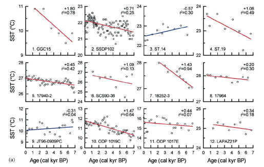
Kim et al 2004 Fig. 1. Caption: (a) Data points (open circles) and linear trends of alkenone SST reconstructions from the North Pacific realm. The magnitudes of SST change over the last 7000 years (1C/7 kyr) are indicated in the upper right corner and the core names are given in the lower left corner of each panel. The numbers refer to Table 1. r is the correlation coefficient.
References:
Kim, Jung-Hyun; Rimbu, Norel; Lorenz, Stefan J; Lohmann, Gerrit; Nam, Seung-Il; Schouten, Stefan; Rühlemann, Carsten; Schneider, Ralph (2004): North Pacific and North Atlantic sea-surface temperature variability during the Holocene, Quaternary Science Reviews, 23 (20-22), 2141-2154, doi:10.1016/j.quascirev.2004.08.010
Stephan J. Lorenz, Jung-Hyun Kim, Norel Rimbu, Ralph R. Schneider and Gerrit Lohmann, 2006. Orbitally driven insolation forcing on Holocene climate trends: Evidence from alkenone data and climate modeling. PALEOCEANOGRAPHY, VOL. 21, PA1002, doi:10.1029/2005PA001152, 2006


17 Comments
Here’s the code:
This coastal core has a rather complex history. It was brackish & estuarine till 6kBP, so the MWP and the early Holocene may not be directly comparable.
#2. Richard, thanks for the reference – the abstract says:
Maybe someone can help me with a slight programming problem. If you go to the link shown above http://doi.pangaea.de/10.1594/PANGAEA.438838, you can download an ASCII file to your computer and then read the ASCII file into R as I’ve done. However R can read directly from URLs – I couldn’t figure out a URL that could be used. I tried various permutations and combinations and then gave up. It’s not too hard to simply copy 40 tables manually, but it’s annoying.
That top graph is like a graph of human history. You can clearly see the dawn of civilization and the long years of the fertile crescent’s golden age. The sudden fall at the end of the golden age of Greek civilization. The mini revival during the Roman Emprire. The Dark Ages, then the gradual recovery from them until ~ the 30 years war. Then the upheavals of the LIA, followed by …… (!)
RE: ~4.3 KYR BP – An event with global impacts, which led to the various great flood tales?
#4
Try http://doi.pangaea.de/10.1594/PANGAEA.438838?format=textfile
as the url
Mr. McIntyre:
http://doi.pangaea.de/10.1594/PANGAEA.438838?format=textfile&charset=ISO-8859-1
They used a hidden form.. had to read the page source.
This worked for me.
http://doi.pangaea.de/10.1594/PANGAEA.438838?format=html
#7 worked for me. Thanks. #9 gets the htm commands which you don’t want and aren’t in the text file.
It doesn’t look like the other cores show much of a MWP. Maybe the resolution is too low??. However, several, including one with a fairly high resolution show a definite spike around 2000-2500 years ago. Roman Warm Period?
Re #2
RichardT, could you explain why the 3 distinct periods may not be directly comparable? The graph would imply that the authors of the paper thought differently or at least I could not find their warning of the complications.
Steve M, when I first read the Lorenz paper I found the trend lines confusing to the point of losing important details of the temperature anomalies flucuating over the time period presented. I take it that these graphs with trend lines represent the tropical areas that supposedly went against the Holocene Maximum to present cooling trends in the extratropic areas. Those graphs that appear to extent into the current times all show maximum temperatures that occur before present times. That perhaps is not what Lorenz was attempting to show — thus the trend lines distraction.
#12. I’m more inclined to attribute a difference between the Atlantic and Pacific from this data than between tropics and extratropics. Once you start trying to come to grips with individual ocean cores, it’s a big undertaking to control all the data (although that’s something that I don’t mind trying to do). AR4 does not review (barely mentions) the recent work on ocean sediments, which is too bad. About the only mention is the use of Lorenz et al for their POV claim on the Holocene Optimum.
Re: #13
I was confused by my laziness not to check the Kim graphs with those in Lorenz (2006). I thought they overlapped but on checking back to Lorenz I see that only two graphs were in common (ODP 1019C and 17940-2). Actually the graphs are presented with Kim starting at present and Lorenz starts in the Holocene time. I have to take back my comment that they were from the Lorenz and showing tropic/extratropic differences.
While some of these plots (both from Lorenz and Kim) show almost linear drops or rises from the Holocene to presnt or near present, others do show significantly more oscillations indicating that one may not be able to attribute the lack of resolution to the general method.
Re: #14
Before I become too apologetic, I must submit what I found on further investigation of the core samples (alkenones) used in the Lorenz et al. (2006) and the Kim et al. (2004) papers. Looking at the cores identified specifically in the Lorenz paper and comparing them with those in the Kim paper I found 15 of 20 identified in the Lorenz were also indentified in the Kim paper. When I finally looked at the source of the core samples used in both papers (Lorenz et al. (2006) and Kim et al. (2004)) I found they all came from Kim and Schneider, 2004. So both papers use the same core samples, but use them in different ways to make somewhat different points. These core sample papers remind me some of the papers produced by the Mann and progeny temperature reconstructions.
#12
As the abstract indicates, this core has only been influenced by the warm Tsushima Current after ca. 4.5 cal ka BP. Prior to this it was in estuarine conditions, perhaps influenced by the coastal current. So while the alkenones may reliably record the SST at this site, the oceanographic conditions at the site have changed.
Re #16
RichardT, thanks, I can now understand your point. The abstract points to the modern marine environment starting about 5.1 kyears BP in this ocean area, which I would assume would make intra comparisons during this time period more legitimate. I know that Steve M has commented about the upwelling regions of some of these core areas as being problematic. Do you have other references giving details of the oceanic history of other individual core areas used in the Kim and Lorenz papers?