One of the Team’s more adventurous assumptions in creating temperature histories is that there was an abrupt and universal change in SST measurement methods away from buckets to engine inlets in 1941, coinciding with the U.S. entry into World War II. As a result, Folland et al introduced an abrupt adjustment of 0.3 deg C to all SST measurements prior to 1941 (with the amount of the adjustment attenuated in the 19th century because of a hypothesized use of wooden rather than canvas buckets.) At the time, James Hansen characterized these various adjustments as “ad hoc” and of “dubious validity” although his caveats seem to have been forgotten and the Folland adjustments have pretty much swept the field. To my knowledge, no climate scientist actually bothered trying to determine whether there was documentary evidence of this abrupt and sudden change in measurement methods. The assumption was simply asserted enough times and it came into general use.
This hypothesis has always seemed ludicrous to me ever since I became aware of it. As a result, I was very interested in the empirical study of the distribution of measurement methods illustrated in my post yesterday, showing that about 90% of SST measurements in 1970 for which the measurement method was known were still taken by buckets, despite the assumption by the Team that all measurements after 1941 were taken by engine inlet.
(Note – May 2008): see current discussion here and Dec 2007 post here
I first discussed this matter nearly two years ago here (see also here) in which I quoted Folland and PArker 1995 as folows:
Barnett (1984) gave strong evidence that historical marine data are heterogeneous. He found a sudden jump around 1941 in the difference between SST and all-hours air temperatures reported largely by the same ships. Folland et al. (1984) explained this as being mainly a result of a sudden but undocumented change in the methods used to collect sea water to make measurements of SST. The methods were thought to have changed from the predominant use of canvas and other uninsulated buckets to the use of engine intakes. Anecdotal evidence from sea captains in the marine section of the Meteorological Office supported this idea. ..
The first quantitative corrections to SST data were tentatively indicated by Folland and Kates (1984), and were closely followed by those of Folland et al. (1984), who applied a constant positive correction of 0.3 deg. C to all data before April 1940, one of 0.25 deg. C to data between April 1940 and December 1941, and no correction thereafter
Folland and Parker justified the abrupt adjustment as follows:
The abrupt change in SST in December 1941 coincides with the entry of the USA into World War II and is likely to have resulted from a realization of the dangers of hauling sea buckets onto deck in wartime conditions when a light would have been needed for both hauling and reading the thermometer at night. The change was made possible by the widespread availability of engine inlet thermometers in 1941 (section 4)
Parker et al 1995, a companion article, describes the situation in similar terms:
Comparison with NMAT suggested that the change in instrumentation took place rather suddenly around the Second World War, so Folland et al. (1984) added 0.3 °C until early 1940, 0.25 °C thereafter through 1941, and nothing subsequently.
Hurrel and Trenberth 1999 describe the SST adjustment as follows:
An additional problem with SST is that it is not as well defined as is desirable. Historically, SST has referred to a bulk near-surface ocean temperature measured by tossing a bucket over the side of a ship in order to obtain a water sample. The design and insulation of the buckets has changed with time, however, so that corrections must be applied (Folland and Parker 1995). During World War II, moreover, there was a switch from bucket measurements to measuring the temperature of water taken on to cool the ship’s engines. These temperatures depend on the depth (3 to 7 or more) and size (10 to 51 cm in diameter) of the ship’s intake, the lading of the ship, the configuration of the engine room and the point where the measurement is taken. Such differences are responsible for some of the noise in the SST measurements, but biases also arise because heat from the engine room more than offsets any cold bias from the depth of the intake. Overall, the differences between engine intake and bucket temperatures is typically 0.3°C (see TCH for a more complete review).
The hypothesis of an abrupt and universal change in SST measurements seemed bizarre from the first time that I read these sentences. In my earlier post, I said:
The idea of an abrupt changeover seems a little weird to me. I’ve also seen reminiscences of an oceanographer [Stevenson] talking about taking measurements in a research ship with steel buckets in the 1950s, so I’m not sure how realistic this assumption is. If the changeover were phased in, it would presumably have a material impact on the SST history. It seems like an important enough issue that it shouldn’t be glossed over.
No climate scientist at the time seems to have bothered determining whether this hypothesis of sudden and universal change in measurement techniques could be substantiated in records. Now Kent et al 2007 have carried out a long overdue analysis of the metadata and reported that over 90% of SST measurements in 1970 for which the measurement method was known were still being carried out by bucket, as shown in the following figure. (While half of the measurement methods are unknown, I see no reason to assume that the distribution of measurement methods would differ materially from the very large sample for which measurement methods are known.
Figure from Kent et al 2007 showing SST measurement method.
The Folland and Parker hypothesis of abrupt and universal change in SST measurement methods in 1941 has been adopted in many data sets. For example, the British GOSTA Atlas 8 (an update of MOHSST6) states that:
The bucket corrections for the SST data are from Folland and Parker, 1995 (see Ref. 1). T
The MOHSST5 (Atlas 7) data, in which the Folland and Parker bucket adjustments are already embedded, was used in the Kaplan’s “optimal estimation” , which says:
Kaplan SST Description: This analysis uses present-day temperature patterns to enhance the meager data available in the past. Reduced Space Optimal Estimation has been applied to the global sea surface temperature (SST) record MOHSST5 (ATLAS7) from the U.K. Meteorological Office to produce 136 years of analyzed global SST anomalies (with regards to normals of 1951-1980) , where data gaps are removed and sampling errors are diminished.
Folland was a lead author of IPCC TAR. The coordinating lead authors of the section discussing Folland’s bucket adjustments are Trenberth and Jones. IPCC AR4 cites several references on buckets and several articles by lead author Kent, but does not discuss this important article. 4AR mentions buckets on no fewer than 10 occasions, saying:
A combined physical-empirical method (Folland and Parker, 1995) is mainly used, as reported in the TAR, to estimate adjustments to ship SST data obtained up to 1941 to compensate for heat losses from uninsulated (mainly canvas) or partly insulated (mainly wooden) buckets…..
recent studies have estimated all the known errors and biases to develop error bars (Brohan et al., 2006). For example, for SSTs, the transition from taking temperatures from water samples from uninsulated or partially-insulated buckets to engine intakes near or during World War II is adjusted for, even though details are not certain (Rayner et al., 2006).
…Owing to changes in instrumentation, observing environment and procedure, SSTs measured from modern ships and buoys are not consistent with those measured before the early 1940s using canvas or wooden buckets. SST measured by canvas buckets, in particular, generally cooled during the sampling process. Systematic adjustments are necessary (Folland and Parker, 1995; Smith and Reynolds, 2002; Rayner et al., 2006) to make the early data consistent with modern observations that have come from a mixture of buoys, engine inlets, hull sensors and insulated buckets. The adjustments are based on the physics of heat-transfer from the buckets (Folland and Parker, 1995) or on historical variations in the pattern of the annual amplitude of air-sea temperature differences in unadjusted data (Smith and Reynolds, 2002). The adjustments increased between the 1850s and 1940 because the fraction of canvas buckets increased and because ships moved faster, increasing the ventilation.
If 90% of known SST measurements in 1970 were still being made by buckets, then the most reasonable estimate for the entire population is that 90% of all SST measurements were still being made by buckets in 1970. This has a couple of implications. First, the adjustment for engine inlets needs to be phased in after 1970 rather than instantaneously in 1941. Dare one wonder whether some portion of the post-1970 increase in SST can be attributed to the increased proportion of engine inlet measurements evidenced in Kent et al?
Secondly, the hypothesis of an abrupt change in SST measurement methods was introduced in order to deal with some real phenomenon. If there was no abrupt and universal switch to engine inlet measurements, then whatever the phenomenon was remains unexplained.
It will be pretty easy to do a first-pass sensitivity analysis of an SST series in which the Pearl Harbor adjustment for introduction of engine inlet measurements is phased in after 1970 rather than in 1941, but it’s not too hard to picture the result.
UPDATE: Here is a first-pass analysis of the impact of a more plausible introduction of engine inlet measurements, as discussed in comments below (see especially #14, 19 and 55). Carl Smith commented:
Eyeballing Willis’s graph, and ignoring the red line, it looks to me like the WWII records were dominated by engine-warmed intake data, perhaps because the chaos meant much of the bucket data did not get recorded, and after WWII it was business as usual with mostly bucket data resuming.
Let’s suppose that Carl Smith’s idea is what happened. I did the same calculation assuming that 75% of all measurements from 1942-1945 were done by engine inlets, falling back to business as usual 10% in 1946 where it remained until 1970 when we have a measurement point – 90% of measurements in 1970 were still being made by buckets as indicated by the information in Kent et al 2007- and that the 90% phased down to 0 in 2000 linearly. This results in the following graphic:
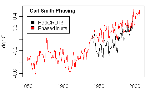
Black – HadCRU version as archived; red- with phased implementation of engine inlet adjustment
Reference: D. E. Parker, C. K. Folland and M. Jackson, 1995, MARINE SURFACE TEMPERATURE: OBSERVED VARIATIONS AND DATA REQUIREMENTS, Climatic Change 31: 559-600 here
C. K. Folland and D. E. Parker, 1995, CORRECTION OF INSTRUMENTAL BIASES IN HISTORICAL SEA SURFACE TEMPERATURE DATA, Q.J.R. Meteorolol. Soc. 121, 319-367 here
Kent et al. 2007 url


85 Comments
Now, I’m not a marine operating engineer (I have a BIL who was; maybe I should ask him about these things) but there appear to be three distinct sources for temperature measurement:
1) Hull (as indicated in the Figure from Kent et al 2007),
2) engine (cooling) inlet (this might well be at the end of a tube feeding a heat exchanger or the water jacket as on a 3-progressive-stage steam piston engine as on a Liberty ship) and
3) bucket.
Does Hansen still agree with himself? Why did the total number of measurements start to collapse after 1990? Is it because their funding was multiplied by 10 after 1990, from $180 million to $2 billion in the US? 😉
Do I understand well that their adjustment is attempting to make the pre-war era look cooler, in order to increase the total amount of warming according to the graphs?
Lubos, good to hear from you. No, the adjustment goes the other way:
w.
LuboÅ¡, this one isn’t Hansen’s baby. This starts with CRU and Hansen criticized HAdCRU adjustments in the early going as ad hoc and of dubious value, as I posted before. Hansen himself seems to be more involved with station data than with SST data.
So, if I understand correctly, 0.3 degrees has been added to the pre-1940 SST measurements because buckets (wooden or canvas) evaporate as they sit on an open deck and hence make the SST seem lower than it really is.
However, it seems the switch from buckets to inlet (and hull) measurements did not take place abruptly in 1940/1941 as previously believed. Phase-out of buckets has been gradual, with 90% of the measurements in 1970 still being by bucket, down to about 10% today (just eyeballing the figure from Kent).
So really, if you’re going to add 0.3 to SST measurements pre-1940, you really have to do it to all measurements pre-1970, and then phase the adjustment out over the next 35 years. That will have the effect of largely flattening the SST record, ie no SST warming?
Yes, Interested, but it’s not that simple, as I remarked in another thread, Parker says:
Nothing in climate science is simple …
w.
There must be some retired mates and seamen in merchant marine associations who remember that they measured temperature by X method between 1950-56 on the good ship Minnow. I suspect a evidence exists to pin down the method used on a lot of those “Unknown” samples, if ship name is listed and the guys writing papers about the data bothered to ask somebody who worked in private industry.
Even a poll of retired merchantmen, while unscientific, would be of interest.
The oft-quoted 0.3C adjusment is 150% of the total increase in SST on a ten year average between 1940 and 2000. My impression is that if the uncertain adjustments amount to a significant percentage of the change in tempeature, the comparison of data sets is spurious and of little value.
Wouldn’t it be the most reasonable to add 0.3 C degrees to any and all temperatures taken by bucket, and leave all intake measurements untouched? Presumably this is what is being done anyway, given that the original adjustment for bucket vs. intake data was done by comparing a period of overlap.
Secondly, with regards to Willis Eschenbach, what is that “bias corrected” graph you posted in the comments? Why is the correction so much greater during the 1900-1950 period than for earlier on?
This site: http://icoads.noaa.gov/advances/folland2.pdf shows a very interesting powerpoint talk by Folland on the topic. It includes pictures of the various buckets (slide 6), and the methods used to calculate and verify the correction. Slide 4 shows a power spectrum of yearly temperature anomalies, and the inset to that figure in particular looks to show a sudden change in the measurement noise level right at about 1941. I’d expect that exact datum is the rationale for the assumed sudden change-over to engine inlets.
Also interesting to me is that the equation they used to model cooling, slide 9, included nothing of the diffusion distance from the point of measurement to the surface or to the bucket walls. The calculations and measurements indicate a surprisingly (to me) large change in the temperature of the water prior to measurement, due to evaporative cooling. Obviously for a given exposure time, and prior to equilibrium, the measured temperature would depend on where in the water one puts the thermometer. Surface water cools much more rapidly than water at the center of the bucket, assuming that the water is not rapidly stirred. I’d want to know where in the bucket the measurments were made to verify the equation used to model the applied correction.
If someone was leaning over the side of a moving ship throwing out a bucket on a line, I’d expect it shouldn’t take more than about 2 minutes to get a temperature. If the bucket were dragged at sampling depth for a few minutes before extraction, the walls of the bucket would have come near the ambient water temperature, slowing heat loss from the captured water.
It also seems peculiar to me that they’d use uninsulated canvas buckets, because canvas is known to keep water cool by evaporative transfer, even in hot climates. Hence its use in canteens. That would have been common knowledge, making the choice of uninsulated canvas to seem pretty foolish. But they weren’t foolish people. So, maybe the canvas wasn’t uninsulated. If you look at the UK Met MkII canvas bucket on slide 6, it has a hard cap of some sort with a small hole for the thermometer. That shows attention to the problem of surface evaporation. Why would they try to minimize evaporative cooling at the surface while nearly maximizing it at the walls by use of uninsulated canvas? That leads me to observe that the canvas walls of the bucket are upright and supporting the hard cap. How are they doing that without internal bracing? Is there an insulating and structural liner inside the canvas? The canvas walls of the MkII bucket look like they are covering some sort of cylidrical inner structure. Is there an solid bucket beneath the canvas?
#6
I think I have to agree with you 🙂
Here are the reported bias uncertainties for HadCRUT3 global average (data , and code , set SMOOTH=0) )
Brohan et al:
zero over normal period? And is the asymmetry due to urbanisation uncertainty ??
Let me see if I understand this: In 1970, 90% of all measurements were still conducted using the “bucket” method that was in use before 1940. Therefore it seems safe to assume there was no more than a 10% shift from bucket to intake measurements in 1940. If we make the exteme assumption that the entire 10% shift in measurement method occurred in 1940, it is easy to show that the estimated change in “bias” of 0.3 degrees C corresponds to a 3 degree difference between the “bucket” bias and the “intake” bias. Following this reasoning, between 1970 and 2005 (by which time the “bucket” method seems to have largely disappeared; for now we can neglect the change in true SST, which was likely on the order of half a degree), one would have expected an increase in reported SST of greater than 2 degrees C.
I agree with Hansen and SteveM. Something is not right.
Dear Willis, thanks for your key answer and nice to see you here! Well, it is ambiguous what is the political sign of such an adjustment. The previous data showed a large jump in temperatures before the post-war-boom that could also be inconvenient because it indicates that it could have been natural. 😉
I don’t know how to find out whether they used buckets and what kind – if others can’t find it. But note that with 2-3 more adjustments like that, one can eliminate the 20th century warming altogether. The very concept of a warming at the century scale – even before we ask about the anthropogenic origin – is still kind of shaky. If you call the adjustment to give you a “sigma” in this jump, the warming is a 2-3 sigma effect which is not an overly reliable statistical result.
Eyeballing Willis’s graph, and ignoring the red line, it looks to me like the WWII records were dominated by engine-warmed intake data, perhaps because the chaos meant much of the bucket data did not get recorded, and after WWII it was business as usual with mostly bucket data resuming.
Just an unsubstantiated idea … but food for thought.
#10 I didn’t read Folland’s paper but this Powerpoint is instructive enough. It shows how you can become so engrossed with theory and models that you believe your own crap. Had I reviewed such a work, I would have rejected it right away. If that is how corrections are applied to the temperature records, we are in deep trouble.
Just look at how the model fits with the (apparently quite old) actual measurements. The difference can be as high as 0.4C one way or the other. I think you actually need to go out on a ship with various models of buckets, along with the most accurate temperature measurement system available, sail across the oceans for a year, take systematic measurements with the different methods, and THEN draw conclusions. THAT is what is called the experimental method. And note that it would still be fraught with uncertainties, because we know nothing about how uniform the taking of measurements has been over the years.
To conclude, as they did, that the correction is EXACTLY and UNIVERSALLY 0.3C before 1941, and EXACTLY and UNIVERSALLY 0C after that is the summum of scientific incompetence! That they validated their conclusion with the use of climate models is also really awkward.
Gee, when you start digging into that stuff, it’s really depressing!
#14
Remove bucket corrections, and correct the WWII effect. Hey, that would give a good linear trend from 1900-present. And no need for aerosol forcing. IPCC fifth assessment: due to improvements in the quantitative estimates of SSTs and aerosols, we have stronger evidence of human influence on climate .
Also notable, the immense crash in sample size since 1985, yet another effect of the amazing consolidation in marine business (mostly due to containerization) and huge drawdown in Western navies. Fewer, larger ships, taking far fewer measurements.
has anyone done a study on the accuracy of the recordings? how accurate are the recording devices and how accurate are the people entering the data. what rank and skill was the crew member hauling buckets of seawater up the sides of a tanker and taking readings? did anyone verify the readings? what quality controls were in place to verify the data recorded in the logs was correct? anyone calibrate bucket readings with intakes? my experience offshore was the crew had a vested interest and great pride in running their machinery well. record keeping was considered an unnecessary routine for idiot bosses. bogus data was occasionally thrown in to confuse others so only the crew knew how to operate their areas properly.
so we have data that was recorded by unknown people with unknown accuracy and we’re debating a fractional degree change in temperature that could result in transforming world policies?
#2,3. I’m focusing on a different issue here. I’m not discussing the merits of the Folland canvas-wooden bucket adjustment pre-1941, but the schedule of the implementation of the engine inlet adjustment.
Let’s hypothesize that Folland has somehow got unbiased estimates of SSTs prior to 1940 and has unbiased estimates at present (say from 2000 on) on the basis that buckets are no longer being used. Now let’s suppose that, instead of an abrupt and universal introduction of engine inlet measurements in 1941, we had a phased introduction so that 90% of measurements in 1970 were still being made by buckets (as indicated by the information in Kent et al 2007) and that the 90% phased down to 0 in 2000 linearly; and that half of the 10% engine inlet introduction (5% of the total) occurred in 1941 and the balance linearly between 1942 and 1970.
As a very quick first pass at ballparking what the effect was, I used the above implementation on the HadCRUT3 global average (I realize that there’s land data in this, but I was using this series in connection with testing a point made by UC and it was handy for me – if I do more work on this, I’ll tidy this up.) The result of this was totally different than the point made by Willis above. It results in much higher temperature estimates through the 1940s and 1950s with an impression of virtually all of the temperature increase taking place by 1940 and little change for the next 50 years. I’m posting this as a comment because I’m experimenting with this still.
Black – HadCRU version as archived; red- with phased implementation of engine inlet adjustment
Here’s the calculation (US has an interesting comment on this HAdCRUT3 dataset BTW)
Let’s suppose that Carl Smith’s idea is what happened. I did the same calculation assuming that 75% of all measurements from 1942-1945 were done by engine inlets, falling back to business as usual 10% in 1946 where it remained until 1970 (when we have a measurement point) going to 100% engine inlet by 2000 as above. This results in the following graphic:
Black – HadCRU version as archived; red- with phased implementation of engine inlet adjustment with allowance for WW2 practices as noted above.
The composition of maritime shipping changed somewhat rapidly
in the early 1940s. Over 200 ships were sunk in 1939, over
1000 in 1940, and over 1200 in 1941. http://www.usmm.org/ww2.html
More gradually, new kinds of ships, and newly trained mariners,
were afloat.
IIRC, shipping lanes changed as a result of the war, perhaps suddenly.
From the graph in comment #3, it appears that the upward
spike near 1941, was followed by a downward spike after the
war ended.
Give me a break. Heat transfer is not this fast in a bucket of any kind, especially a wooden bucket, given the insulating properties of wood. I could see a change on 0.3 C if the guy doing the measuring had a couple of beers between hauling the bucket on board and measuring the temperature. But not in 5-10 minutes!
#15
You say that no-one cruised the oceans with recent temperature probes and historical buckets to get the correction factors right?
#11. Futher to UC’s interesting identification of HadCRUT3 uncertainties being archived, here is my plot of the uncertainties from the HadCRUT3 archive:
, “Bias” here is essentially bucket adjustments. It’s pretty amazing that they think that the uncertainty for bucket adjustment is less in 1865 than in 1938. They assume uncorrelated errors.
Here’s the retrieval and calculation (thanks to UC for the template in Matlab from which I’ve varied a little here ) –
##HAD Uncertaiunes
## see U: http://www.geocities.com/uc_edit/hadcr3.txt
#17
Has anyone tried contacting any retired Areographers Mates who served from during the last 30 or 40 years? When I was going through the DOD Weather Schools in the early 80s I was under the impression that the Navy took SST samples from buckets. I know the US Navy represents only a fraction of the overall shipping, but thier weather observers were usually top notch, and thier supervisors ensured good quality control. Remember, SSTs info was/is extremely important to the war time survival of thier subs. I haven’t been able to get any online info on how the Navy collects its surface ocean temps, let alone any historical information.
Question: are the official SST estimates still made using surface thermometer observations?
I’ve been under the impression that since about 1982 SST is based on satellite estimate of surface temperatures. I’ve viewed the SST record as a graft of satellite data onto thermometer data during the 1980s.
Complex.
I wonder if the geographical distribution of the SST measurements taken after the Pearl Harbour attack is the contributing factor. There were probably more ships in more areas not routinely observed from normal sea lanes.
Could it be that the apparent temperature “spike” during WW II was caused by something other than the bucket issues? For example, since showing lights at night was generally not a good idea because of the submarine threat, maybe the measurements were biased more to daytime measurements, where the surface was generally warmer due to solar heating, than to average temperatures over the whole day which would be more typical of peacetime. Intuitively, this could be a bigger effect than the bucket vs. inlet effect, and would naturally go away when the submarine threat did. It would seem to me that a concerted effort should be made to find seamen from the WW II era to help understand this before they are all gone.
The WW2 situation is interesting, but there are many years between 1946 and 1970 that are unaffected by night light issues. Whether or not one makes a special adjustment for WW2 values, I can’t see any basis for assuming that 100% of 1970 measurements were engine inlet measurements in the face of Kent et al’s results. Nothing more is needed to disprove the Folland hypothesis.
The biggest threat of WWII and and after it was submarines. As sonor depends in ocean temperature it is much more likely that the USN started making damned sure that they knew the real water temperature when they went hunting for U-Boats and Soviet subs. This is also they time that the USN started spending much more time being interested in the weather, the Pacific fleet hit two typhoo’s in 1944-45 losing more than 800 men. After this they wanted to be able to predict the weather. It was very important to know if you should go ahead and refuel or to ballast with seawater if there was going to be a big blow.
#24
Note that it can be some kind of UHI uncertainty as well (http://hadobs.metoffice.com/crutem3/urbanisation_change.html). Probably nobody knows. And note the additive uncertainty formula that seems to reproduce Brohan Fig 10 :
sqrt((e1l).^2+(e2l).^2+(e3l).^2) % blue
sqrt((e1l).^2+(e2l).^2) % green
e1l % red
Switch the order, e1l,e3l and the bias errors will become more visible. Maybe I have misunderstood what is going on, but hypothesised distribution of the adjustments required in Figure 4. gives a strong indication that it is not me.
#25, #26
There are more than six methods which may be used to measure and report surface sea temperatures. The WMO provides guidelines to the member national authorities. Most of the surface sea teperatures reported to the National Weather Service, NOAA, Dept. of Commerce, United States originated from voluntary ship observing program/s. For an example, see:
http://www.nws.noaa.gov/wsom/manual/archives/NB309204.HTML
U.S. DEPARTMENT OF COMMERCE
National Oceanic and Atmospheric Administration
NATIONAL WEATHER SERVICE
Silver Spring, Md. 20910 August 26, 1992 W/OS0141:MB
MEMORANDUM FOR: All Holders of Operations Manual
SUBJECT: Transmittal Memorandum For Operations Manual Issuance 92-4
1. Material Transmitted:
WSOM Chapter B-30, Voluntary Observing Ship Program.
2. Summary:
This chapter describes the operating procedures and administrative structure of the National Weather Service (NWS) Voluntary Observing Ship Program. This program is the primary means by which the NWS obtains surface observations from marine areas. Revisions to instructions and procedures are present throughout the chapter.
[….]
Exhibit B-30-A3: WS Form B-31, Code Entries for Data Field
(page 3 of 10)
Card 1
CARD
COLUMN FIELD
HEADING DATA FIELD
[….]
46 Sea Surface Temperature Method
CODE 1 Thermometer in condenser intake
2 Bucket thermometer
3 Hull sensor
4 Tank thermometer
5 Infrared sensor
6 Other
From Kent et.al 2007:
So I’m prompted to wonder… Since 1970, fewer, larger ships reporting SST from fixed (intake/hull) sensors – could this intruduce a warming bias in the recent observed SST data?
#33
If, in fact, it is ever demonstrated that there was any significant bias or errors in the VOS SST observations, there would then also follow certain consequences to the accuracy of those satellite observations, which used the in-situ observations of the VOS network to calibrate the satellite data for atmospheric absorption coefficients. Opportunities for the incorporation of bias and errors into the satellite data sets and the Comprehensive Ocean Atmosphere Data Set (COADS) relied upon by the IPCC and NOAA begin with the methods used to average the raw data observations from sea station observations in the VOS network into one and five degree regions. However, the VOS network coverage was quite limited in coverage and quantity of data, so the more recent NOAA/NASA Pathfinder Project data has been used in conjunction with the base data of the VOS network back to 1942 to compute interpolated data for the earlier periods in the time series. Any observational inaccuracies in the actual observations of the VOS network and their computed averages may consequently become magnified many-fold (hundred-fold?) by the foundational VOS-Pathfinder assumptions and calculations.
It has been noted by investigators that the algorithms used for adjusting satellite observed SST data has been inconsistent, cloud coverage has limited the adequacy of satellite coverage, and in-situ measurements by VOS and buoy networks has been inadequate with respect to the datasets produced by the Advanced Very High Resolution Radiometers (AVHRR), Cross Product Sea Surface Temperature (CPSST), Non-Linear SST (NLSST), and Multi-Channel Sea Surface Temperature (MCSST) methods. Yet, the IPCC, certain NOAA and NASA proponents, and others in the climate science community purport the products of these methods are accurate enough to support their conclusions and climate modeling.
Are they, or is this perhaps another case where faulty assumptions, algorithms, analyses, data products, and peer reviews have resulted in non-scientific conclusions?
A fascinating discussion. In my many years at sea in HM Navy, I could never have anticipated this! Some unconnected observations:
1. Almost invariably, seawater temperature was taken from a thermometer set into the main inlet providing cooling water to the condensers used to condense feed water used in the ships’ boilers. To obtain the temperature, recorded once a watch of 4 hours, the Officer of the Watch would have the engineroom called to report sea water temperature. N.B. no mention of SST here – just the “seawater temperature”. The depth of the inlets would vary with ship size, but the inlets were always near the bottom of the ship and thus typically 15 – 25 feet below sea level. The reasons for this recording remains obscure to me, but it could have been to keep a check on the relative air and sea temperatures and hence the possibility of fog. A sudden change in either could presage development of fog. The engineroom’s interest was in efficiency of the plant – warm seawater meant less efficient condensation and limits on power available. I guess that diesel engines would have had similar outcomes, but I don’t know.
2. Accurate sea temperature was much more important in anti-submarine warfare where, in order to predict likely detection ranges of submarines from a surface ship, it was critical to have temperatures at all depths to which a submarine could operate. These were obtained from a bathythermograph which produced in graphical form a vertical slice of depth v temperature. There were often layers of water of similar temperature to a certain depth until a sudden change to colder water would occur. Thereafter the temperature usually declined uniformly with depth. Knowledge of these layers was very important as a surface layer could trap sonar emmissions, reflecting them back to the surface. Any submarine (which also knew the temperature profile) could then adjust his tactics accordingly. Bathythermograph readings invariably included a bucket reading of the SST. This was taken via a metal bucket (2 gal!) on a rope and a nimble able seaman to recover it. It would have taken a sample from about 2 – 3 feet. Immediately on recovery, a very sensitive thermometer would be used and SST recorded. The effect of surface “mixing” was always important as this would decrease the chance of a surface layer developing. “Mixing” was caused by rough sea conditions. Calm, hot days as found in the tropics were a submariners dream as the surface layer became more and more established. As an aside, getting below the layer with sonar was achieved by the development of the towed active sonar.
3. Sonar really came into its own as late as WW2. Awareness of the importance of accurate SST may have developed in this time. It’s a long shot, but possibly worth chasing down.
4. Finally, I find it astounding that such accurate SST results could have been derived from such crude records which themselves came from some pretty rough and ready techniques and instruments, at least prior to WW2.
Look, this is a silly argument. If you all are correct, there will be an upward bias after 194x (where x is the end of WWII) and SST will still have an upward trend. Won’t look as bad, but it will still be there. Kent, et. al. 2007 made no recommendations as to how an overall bias correction should be made, but did point out the difficulties of normalizing SST, wind speed, temp, barometric pressure, etc. The metadata is just too fragmented to make this an easy job. Kent, et. al., was an attempt at merging the available metadata to sort out the puzzle, but admits that this is a very difficult job.
Now you may be wondering why this has not been done up until now. My guess is that it is a very painstaking and boring job, and may well not result in a major change in the Folland corrections, which are probably good to a first approximation. She has pointed the way to get a better correction factor, but has not invalidated the currently used correction factor.
Face up to it guys: this is how science progresses.
My understanding is that ships take water temperature readings from where they are. They don’t travel to a particular spot to do the
readings. So how do we create SST trends from readings that are being taken from different spots every time they are taken?
The oceans are not uniform. Even things like the shape of the bottom can affect SST. Mountains and ridges can create localized upwelling.
Whether you are in a current, or outside of it, can in the space of a few hundred feet, mean several degrees of difference. Worse,
currents meander a bit. The location of their edges change from day to day.
#35
How interesting! To live is to learn… 😉
#36, jms,
knowing the variables discussed here, do you believe there is enough precision in the data to assert there is a fractional degree rise in ocean temps over the past 150 yrs?
JMS,
The primary driver of science is people asking questions and seeking answers. This includes questioning the current “understanding”, which is what we are doing here. It is important to understand the limits of the current theories and data so that we don’t get out onto thin ice with our conclusions. This is our goal here. What’s wrong with that?
Re # 35: Before the advent of GPS navigation, ocean temperature was the principal means by which a navigator could infer that a vessel was encountering a current. Hence the large number of readings. By comparing these with a map of known currents and their ‘normal’ temperatures, the navigator made inferences on the effects of the current.
Paul, that is exactly what you saw in the Kent, et. al. paper. It was a suggestion that the empirical correction may be wrong and that things need to be looked at. Maybe there is a better way to put a bias correction on the data, maybe not. But what is being done now is not dishonest (as Steve so often implies), but an honest attempt to create a bias correction.
What is wrong with what goes on here is that you all seem to be seeking to tear down the science, not build it up.
#JMS, please don’t put words into my mouth. In law, there are many nuances of tort and “dishonesty” is irrelevant to most situations and I didn’t say that the Folland adjustment was “dishonest”. Is it “negligent” that no one checked the validity of the assumption? In some sense, there is a collective negligence on the part of the field, but it’s hard to say that any one individual had a specific obligation of due diligence. The lack of adequate due diligence – and the failure of organizations like IPCC to carry out due diligence – is something that I emphasize again and again. But I didn’t suggest “dishonesty” on the part of Folland. After all, he never claimed that he didn’t have r2 with that statistic.
JMS
Where in what Steve M has posted has he implied dishonesty on the part of Folland et al? I’m finding thios thread very intersting albeit hard to see the punchline at this stage.
Now I know I’m being lazy but so far no one has answered my question in the previous ‘bucket’ thread. What contribution to the overall mean global surface temperature do the land based and SSTs make. Which is dominant in respect of the claimed observed increased post 1975 warming?
It’s very clear (thanks to Steve M, Willis etc) that there are issues with both but given the current hyped claim by the ‘warmers’ that the past effects of man-caused global warming have largely been masked by the warming of the oceans and that unless we reduce CO2 emissions now that we won’t be able to mitigate future global warming when this ‘stored heat’ eventually comes back out of the oceans and leads to catastrophic effects, I’m very interested in getting to the punchline of this debate on SSTs.
Also given the oft quoted phrase by ‘deniers’ that much o fthe 20th century warming occurred prior to 1940 and so before the largest rises in CO2 atmospsheric concentration, I’m interested in knowing what effect these pre-1941 only 0.3C bucket corrections has on the ‘deniers’ claim (recently repeated by Mike Durkin in the Global Warming Swindle Channel 4 documentary).
KevinUK
Re: #44
Most of the spatially averaged global temperature has to come from the oceans and thus the importance of Steve M’s query here. The SSTs should be free of UHI and much less susceptible to uncertainty due to lack of complete coverage, i.e. something we could hang our hats on – then Steve M opens this can of worms.
Excerpted from here.
JMS
Also as I see it at present, those rigorous scientists (the ‘hockey team’) are avoiding the need to ‘update the proxies’ and instead are continuing to rely of the ‘spliced’ hockey stick (un-updated proxies spliced on to ‘dodgy’ measured instrument data) as the primary evidence for AGW. Slowly but surely our resident ‘Toto’ is pulling back the curtain and I predict that it won’t be long now but the Wizard of East Anglia is completely exposed for the eco-theologically inspired charlatan that he is. The soon this happens the better because as far as I’m concerned once this happens I won’t have to pay the ‘green taxes’ which our PM in waiting Gordon ‘Macavity’ Brown chancellor intends to impose on me following the ‘dodgy dossier’ Stern Report he personally commissioned.
KevinUK
#42, JMS
“What is wrong with what goes on here is that you all seem to be seeking to tear down the science, not build it up.”
This is, perhaps, too broad a generalization, but if it were true – So what…
Scientists are supposed to “tear down” the science – That’s the way science works to approximate truth. Scientists don’t prove anything – they come up with lots of ideas and “tear them down” one by one – until they’re left with a most probable explanation.
You can build a fantastic house of cards if there’s no wind around to test it. Paleoclimatology should welcome, expect, and withstand assault from scientists, oil execs, crackpots, and honest skeptics.
Tearing down the science is the way real scientists build up the science.
“eco-theologically inspired”
They may have taken over the cause,
But I was surprised to learn in Swindle
AGW was initiated by Margaret Thatcher,
and the aim was busting the Coal Miners’ Union.
RE: #48 – “AGW was initiated by Margaret Thatcher, and the aim was busting the Coal Miners’ Union.”
Here’s a bit of trivia …. those who are well familiar with the lyrics of Sting’s earlier solo material will recognize that he was inadvertantly part of that meme … Sting aided and abetted Maggie? ’tis true!
JMS says:
I just did a comparison of solar to temperature with the Folland adjustment phased in according to my diagram shown above. It is startling.
#50
OK Steve so show us the chart and hopefully it will become the poster child of the IPCC Fifth Assessment Report.
#48 FTM
It was John Daly who first put forward this theory of how AGW politics all began (in the UK at least) I believe. I used to work in the nuclear industry at the time and can personally testify as to Maggie’s pro-nuclear inorder to defaet the miners motives at the time. Once the coal miner’s were defeated she proceeded to remove her support for the planned ’10 further nuclear power stations’ (and so only Sizewell B was built) and opted for the City financiers inspired ‘dash for gas’ option instead.
KevinUK
#49, Steve,
I hope you’ll point to us the “early solo” material source
But I can think of one relevant in the Police era…
Re # 49,
What is “We Work the Black Seam”?
Never put the two together, as the UK coal strike didn’t get a lot of press in the US.
Re: #44
You should state this correctly even if the warmers get it wrong. There is no ‘stored heat’ and it won’t “come back out” unless the heat input goes down and the temperature decreases. Assuming that there is, in fact, a positive radiation imbalance, heat will gradually stop going in as the ocean warms to balance the increase in radiation by an increase in emission. The time scale of this is decades to centuries depending on how you run the numbers, particularly mixing of the surface with the deep ocean. The enormous thermal mass of the ocean, not to mention the heat of fusion of the polar ice caps, damps the temperature response of the planet to any increase in heat input. Basic physics, the heat capacity of water (and the heat of fusion of ice) is much larger than than that of air or land.
I took the graphic from #19 in which the Folland adjustment was phased in allowing for the fact that 90% of known SST measurements in 1970 were done by bucket and not engine inlet and regressed that against a solar index that I had handy (Lean 1995) and plotted the two series together. Here’s what I got and this is the first pass without any attempt at designing:
The correlation between the two series was 0.80 going from 1850 to 1995, the last year of the Lean 1995 solar estimate. I’ll compare this to Lean 2000 as well. This isn’t a “decadal” correlation or some such either. This is using the annual data.
I should add that high solar correlations were observed in various articles in the early 1990s e.g. George Reid, but the validity of these correlations was contested by IPCC and others due to the fact that a physical basis for the correlations would require a greater sensitivity of temperature to solar than to CO2 “forcing”. I think that I posted up on this in the past, but maybe I just have notes on this. I don’t understand the reasoning by which it is held to be impossible for the sensitivities to be different – after all, solar energy is very short wave length, low-entropy while IR is long wave and high entropy so conceptually different sensitivites seem possible to me, but I haven’t investigated the matter in detail.
RE #56 There’s that odd cyclical behavior in Holgate’s sea level change rate plots, which looks remarkably like it’s in phase with solar activity.
To me, that suggests the possibility of some subtle relationship between solar activity, sea level changes and ocean temperatures changes, but I have not even a wild guess as to how such a relationship would work.
Steve,
I think it is fairly well established that the earth’s climate system is more sensitive to solar forcing than one would expect from a simple back of the envelope estimate of the increase in total irradiance.
For example consider this from Lean’s popular piece in Physics Today, June 2005
There are issues with the total irradiance reconstructions. However, her comments are supported by an array of circumstantial evidence. At the moment, to my knowledge, no one understands climate reponse to small changes in solar irradiance.
— Pete
Steve, exactly how did you adjust HadCRUT3 (better to do only the SST stuff, though)? I don’t see any reason to assume that the “unknown” portion has the same distribution of methods as the “known” portion, more likely the unkonwn portion was done by commercial ships which did not report a method but probably used engine intake temps. The metadata is pretty sketchy and only begins to become thorough during the later part of the period surveyed by Kent, et. al.
Kent points out many confounding factors even in the intake temp, so it is going to be difficult to come up with a systematic bias adjustment (therefore 0C might be a good guess). If you really want to get a good adjustment you are going to have to go through the raw data, identify the ship, the method used and account for things like the depth of the engine intake or hull sensor and do it measurement by measurement. This is not exactly an appealing line of research but, as suggested by Kent, it should probably be done. This seems like a perfect project for an amateur and could probably make an actual contribution to the science by doing it. God knows it is boring and requires enough time and patience to do that no working scientist is likely to try and follow the metadata back through Lloyds to come up with a correction factor; it costs too much and takes a huge amount of time from more promising lines of research.
The bucket correction factors were derived experimentally, so I feel pretty good about the bulk correction factors prior to 1940 and it is an upwards correction, so it should make warming look less alarming. My guess though is that a bulk correction factor of 0C is OK for the post WWII era — deep engine inlet temps vs. corrected surface buckets will probably give a slight cold bias to post WWII temps. Think about it: Kent showed that inlets on various types of ships varied between 5m and 7m. This depth correlates well with Jacko’s observations from his experience in the navy, and if that temp is at the inlet it will be colder than the actual SST.
[TCO mode] There is obviously some work to be done here, but my gut feeling is that it won’t make any difference — OC will be the appropriate correction post WWII. You’ve got the time, do the research. You even know where to find the raw data! [/TCO mode]
Finally, you did criticize the IPCC for not including Kent, et. al. (2007) — although those opinions appear to have been deleted — when you knew full well that the cutoff was in 12/05 for papers in press. NOTHING after 2006 could have been included and you know that. You do have a habit of redacting your more rash statements without indicating that you have edited the post. I consider this to be dishonest.
#59. How did I do the adjustment? I provided a script in #19 above if you care to follow he exact calculation.
The starting point surely has to be the hypothesis that the distribution is the same in the known portion as the unknown portion. You have no evidence for the hypothesis that the distribution would be different. It might very well be, but you can’t assert that it is without any information. This type of assertion is all too common in Team climate science.
There are billions of dollars being spent on climate science. If this data is being used, the details should be done correctly. The people who are being paid to do the work should do the work.
I often write straight to the blog and sometimes edit afterwards. I quite often note when I’ve made changes. You’re right – I do know that the cutoff was in 12/05 for papers in press. Indeed, I’ve commented on this in connection with Ammann and Wahl, which was cited by IPCC 4AR although it was not then in press nor even accepted. Ammann and Wahl was supposedly accepted at some later date, but the version that they filed with IPCC was not the version that was ultimately accepted. I pointed on in an earlier post that Ammann and Wahl failed IPCC cutoffs. As a reviewer for IPCC, I observed formally that Ammann and Wahl failed to meet IPCC cut-off dates. We’ll see whether IPCC 4AR uses it – I’d be shocked if they didn’t (even though it still hasn’t been published nearly 16 months after the cutoff date for being in press.) Also as discussed previously, the version filed by Wahl and Ammann with the IPCC TSU and made available to reviewers was not the accepted version. The accepted version, after a complaint of academic misconduct against Ammann, admitted that the verification r2 of the Mann reconstruction was ~0, a point cited by the NAS Panel. This version was eventually archived with TSU late in the review period only after the issue was raised here.
So, to the best of my knowledge, IPCC did not apply their cut-off rules in a consistent way. I would presume that someone at IPCC was aware of the bucket problems being identified by Kent et al and the issue might have been raised. There were other points that I wished to emphasize in this post and that would be the reason for editing. I might well return to the issue on another occasion though. It’s hard to understand why IPCC would not discuss these issues, if they managed to exempt Ammann and Wahl from their cut-off rules.
#58. Peter, thanks for this. Despite this reference, Hansen has asserted quite categorically that the sensitivities for solar, is if anything, less than the sensitivity for greenhouse forcing. So the issue is hardly settled. Your reference is an interesting one and I’ll try to follow up.
re #57, David Smith says
“There’s that odd cyclical behavior in Holgate’s sea level change rate plots, which looks remarkably like it’s in phase with solar activity.”
In a previous thread I posted this chart which has the sunspot cycle overlaid on Holgate 2007.
Note the X1, X2 comment – there is a five year displacement on the overlay. The relationship is obvious – as to what it means or how it comes about, I have no idea.
RE: graph at 3. Does anyone know what is causing (note the present tense — we now know that the past is still mutable) the spike in SSTs around 1940? Is there some coming together of various uptick drivers which co-incidentally gives this surge? It’s interesting to note how the adjusted data hides the spike, making it much less obvious.
RE: 28. Maybe the spike is real, the data trace of a real temperature excursion. Is there data which indicates whether it’s a NH, SH or whole world event?
The unadjusted graph shows a rather neat continuous rise from around 1910, fluctuating a bit, and a little thermal maximum during the war. The adjusted data is much more difficult to get a handle on — it makes me worry about what other real-world events are hidden by adjustments to various data sets which the naive eye misses.
JF
(You know what I think by now — I think it’s the Kriegesmarine signal. My life would be made perfect by data indicating a similar downward spike in albedo at the same time. It would be nice to compare the 1910-2000 portion against estimated pollution load on the Atlantic as well. I’m beginning to imagine I can see the synthetic surfactant pulse after WWII, so I’d better stop.)
#56,
Sounds like the IPCC is engaged in circular reasoning. They assume a certain level of CO2 forcing, then object when the observed
solar forcing is greater than their assumed CO2 forcing. Declaring it can’t possibly be right, because the observed differs from their
assumed.
Julian (#63),
I’ve been wondering the same thing. As a child, growing up on the East Coast of the U.S. and spending nearly every summer day at the same Atlantic beach, I remember when “beach tar” was ubiquitous (after a day at the beach, you had to use kerosene to get the black goo off your feet). “Old Timers” said that the tar was coming from ships sunk during WWII (which sounds plausible, though I can think of other explanations). In any case, the beach tar began to disappear in the 1970s; you never see it today.
Having read further, am I right in my belief that the bucket correction was applied simply because there was a big temperature uptick around 1940, and instrument error seems a good way of explaining it? This is rather like my claiming that rising ocean levels are inexplicable and there must be something wrong with all the stilling wells. With enough ingenuity I expect it would be possible to do that, but it’s hardly science.
Does anyone know the whereabouts of a detrended SST graph from 1910 to 2007? The data lurks in the graph above, but I lack the skills to reveal it. The trend looks like .14 deg/decade, nice and steady, like the Mauna Loa graph.
Re: 65. It’s amazing how far a little oil goes. Benjamin Franklin stilled a couple of acres on a Clapham Common pond (IIRC) with about five millilitres of oil. When you think how many millions of litres of fuel were spilled during the battle for the Atlantic, the power of mankind to damage the ocean surface, and alter its wave characteristics, is very obvious.
JF
vis-a-vis #61
Assertions aren’t an accepted methodology in my field so it would be interesting to see how he reached this conclusion and deals with the building literature that concludes otherwise. Since you appear to be interested in something more than Lean’s brief popular piece. A good, comprehensive overview of these issues is introduced in
The influence of solar changes on the Earth’s climate
L. J. Grey, J. D. Haigh, R. G. Harrison
Hadley Center technical note 62, January 2005.
Naturally some of this material has been updated, but this provides entry to the literature and issues.
pg. 4
There is also a handy summary and assessment of mechanisms (as of January 2005) on pg 66-68.
— Pete
There is a very simple possible reason for the sudden anomaly in SSTs for 1939 to 1945 – a discontinuity regarding which parts of the ocean were being sampled. On the outbreak of war Britain immediately instituted convoying. Ships no longer followed the great circle routes which minimized distance sailed. They sailed routes dictated by the convoy escort and the Admiralty. the primary rationale for which was avoidance of submarines.
My guess is that on the North Atlantic, where most of the shipping was concentrated, they followed more northerly routes. For one, the departure/arrival point became Halifax versus New York or the gulf of Mexico (tanker traffic). Ships leaving Eastern US ports would have followed the Gulf Stream North. From Halifax, most westerly routes would have taken them along the Gulf Stream too, as opposed to the cold central North Atlantic they would have crossed if they had followed a great circle route from New York, say, or Miami to Liverpool or Southampton or London.
So my guess as to why SSTs went up in WWII is that the ships were diverted to the warmest part of the ocean. Simply put: they were sampling the Gulf Stream.
Conclusion: it is probably a simple case of sampling bias.
RE: #53 – Ding, ding, ding! We have a winnerrrrrrr!
?? Pearl Harbor? But WWII started in Sept 1939. Were all samples taken by American-regd ships only? I don’t understand.
The naval component of WW2 waxed and wained, and the intensity shifts occurred between oceans too. I don’t remember exactly what the most shipping was sunk, but I think it’s likely that very little of it was sunk in the Pacific prior to Pearl Harbour. As for the Atlantic.. I’m pretty sure the submarine war started early, but was much less intense early in the war, before Germany really ramped up their U-boat production. Plus the addition of US shipping when they joined the war made for both more targets and more ships doing the sinking.
So to sum I think you’d have to look at tonnage sunk per month in each ocean to get a really good picture of when such an effect would be expected to become pronounced. If you’re just concerned with sampling effects, you’d need to look at the number of passages in each ocean for each month during that period to look for any spikes, especially those related to the US entering the war.
An extremely informative report by Kent ‘Assessment of Biases in Merchant
Ship Surface Temperatures’ is here. It includes a description of bucket collection methods (with pictures of the various buckets in use) as well as an analysis of error/bias in data collection between bucket/intake methods. Worth a look if you’re interested in VOS reported SST data.
#71 Early in the war, the US depth charges did not have enough explosive power to sink a German submarine. As a result, there were a lot of sinkings by German submarines within sight of the east coast of the US. The development of a method for large scale manufacture of the explosive RDX changed this and soon U-boat missions were far more dangerous and less productive.
Steve N., thanks for the very interesting report by Kent et al.
I found this quote quite revealing:
Kinda puts the end to the “the adjustment was necessary because uninsulated buckets stopped being used in 1941” theory, I’d say.
w.
Then we have this quote from the Kent study:
I think the uninsulated vs. insulate bucket argument is DOA …
w.
Just gets better …
The Parker (1985) analysis forms the basis for the comparisons presented by Folland et al. (1993). They comment that the global difference they found of order 0.1°C might be smaller than those in previous studies due to the use of uninsulated buckets in the earlier studies.
However Walden (1966) obtained a 0.3°C mean bias possibly from insulated buckets similar to the German bucket in Figure 10. Furthermore James and Fox (1972), describing measurements taken in 1968-1970 from buckets of known type, found that the mean difference from engineintake SST for the German bucket was 0.18°C, the Crawford bucket (Crawford 1969) 0.23°C and “other” national buckets 0.25°C.
Re: 68. I think that convoys would have travelled more widely during the war than pre-war traffic, which presumably would have chugged along the great circle routes. Perhaps pre-war particulate emissions caused more cloud along the frequently travelled routes, which would have lowered the temperature — think of it as very low contrails. There’s a picture of ships below thin stratus somewhere on the web which illustrates the effect rather nicely.
But surely someone would have thought of that before plumping for slightly cooled buckets made of wood or canvas — which weren’t actually phased out until the 70s — as the cause of unexpected warming in 1940.
JF
Re #72: a more recent / appropriate report on VOS SST is the Kent and Kaplan (2006) paper.
Kent, E. C. and A. Kaplan, 2006: Toward Estimating Climatic Trends in SST, Part 3: Systematic Biases. Journal of Atmospheric and Oceanic Technology, 23(3), 487-500, DOI: 10.1175/JTECH1845.1
As for the issue of the SST bias correction applied to HadSST2 (which forms the marine component of HadCRUT) Rayner et al (2006) themselves admit that the bias correction is incorrect. Quoting Rayner et al
Re: #55
Here is the same plots on the IPCC TAR global average temperature graph:
Alan
Fascinating …..
I think some of the comments from other threads and even RC is in order. I noted that there were several complaints about Watts looking at the micrositing effects. Several of us had a problem with Hansen stating that UHI was not detected. One of the points made was that with SST, and satellite data, that this supposed small difference in land data(not Watts’ claim) would not have a large overall effect. Now we find potential SST data that while it may not necessarily change some of the total delta C, it could change the shape of the curves that are used for the calibration period. Also, satellite data in and of itself cannot be used without correlating to the surface and now both networks may have problems with them. These are not minor as has been implied or explicitly stated.
As Steve has pointed out in #55, #61 that
Hansen has asserted quite categorically that the sensitivities for solar, is if anything, less than the sensitivity for greenhouse forcingmay be unjustified.#59, #60 IPCC rules allow the use of unpublished but otherwise available papers. ANNEX 2 PROCEDURES FOR USING NON-PUBLISHED/NON-PEER-REVIEWED SOURCES IN IPCC REPORTS If I remember correctly, it is left up to the main authors or chairman of the working Group. So Steve can easily call their hand if it is readily available before the final report writeup is due (about August 2007).
There were several comments such as #21 about the shape of the spike matching WW2. The information in #35, 28, 68, and 30 combined with googling Intercoastal Watterway use in WW2:
One would epect to see temperatures increase if they went to rigorous sampling. It would have occured for many navies in 1941 to 1942 because of the entrance of the US in the war. The great circle route GCR was used. In fact if you read of the original rich farmers in the US, they were a naval society who could easier send their children to Britain using the GCR that even in the US. The large number of Liberty ships in 1941 in resposne to war. I am familiar with this since so many ships were sunk off the coast of SC and NC in WW2 trying to make the trip to Europe. The important point of #35 is if more temperatures are being taken, and historically on the east coast of the US, the ships spent more time in the intercoastal if possible and took paths where the Gulf Stream was warmer, and may have used the Gulf stream for the added effeicency (I remember reading that but could not find it) then perhaps the only part of the data that need to be changed is a .3C decrease for 1941 to 1945.
In several threads it has struck me and many that we should be automatically labeled deniers for considering that the solar effect, or UHI should be at least a significant factor. I don’t where all this is leading, but I can’t help but see it will make the science better. If for no other reason but that the data and assumptions were looked at and found to be correct after rigorous scrutiny.
bump. This is last year’s post that I mentioned.
55 (SteveMc): You used Lean 1995 for TSI. Not even Lean thinks anymore that that reconstruction is valid. Steve, please try not to perpetuate the old TSI reconstructions which we know today are not valid. On my website is a compilation of modern TSI-reconstructions. Use column C (me, the best, of course 🙂 ), D (Dora Preminger, also good), or K (Krivova et al., if you must). The latter still has a unsubstantiated, small background change during 1900-1950.
#83. Fair enough. I’ve spent some time with the different solar versions. It would be worth re-doing this graphic with a new version to see what it looks like.
Awesome post! Seriously you give some top quality high content which is awesome. Thanks for sharing with us and keep it up!
8 Trackbacks
[…] several past posts here here here , I’ve observed that there is a very substantial and speculative adjustment of SSTs for […]
[…] next day, I re-examined the Pearl Harbour hypothesis, carrying out a calculation on the basis of Carl Smith’s […]
[…] showed the prevalence of buckets as late as 1970 (discussed here), I showed in a post entitled The Team and Pearl Harbour that this directly contradicted the Team’s Pearl Harbor adjustment and even showed the impact […]
[…] been originally criticized at CA in 2005 here and further discussed at length in March 2007 at CA here, a post in which I observed that no climate scientist had made any attempt to validate […]
[…] compensazione dell’errore sistematico elaborato da Folland et al. non è esente da critiche. S.McIntyre, in particolare, ne esprime alcune che, personalmente, mi sento di […]
[…] The Team and Pearl Harbor […]
[…] The Team and Pearl Harbor […]
[…] and Engines, The Team and Pearl Harbor, Bucket Adjustments: More Bilge from RealClimate, Rasmus, the Chevalier and Bucket Adjustments, Did […]