As I re-examined the IPCC TAR spaghetti , I noted that there was considerable evidence in Figure 2-21 that the Maestro himself is in the house and we should therefore be prepared for the unexpected.
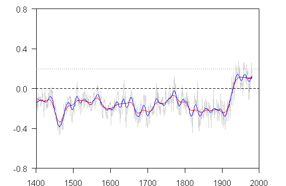
There is an interesting replication problem in the TAR spaghetti graph where I’d welcome ideas. Here’s the TAR spaghetti graph (their Figure 2-21). On the right is a blow-up of the right side, which I’ve shown before. In the blow-up, you’ll notice that the Briffa MXD series and two other dark-colored series come into the blade of the hockey stick, but only two series come out. Hey, it’s the Team and you have to watch the pea under the thimble. The Briffa MXD series in this graphic ends about 1960, In the citation (Briffa 2000), it continues on to 1994 with a very large divergence. But more on this on another occasion. I want to focus on a smaller problem right now.
The smoothing in these series was said to have been done using a 40-year Hamming filter with 25-years end-point padding. Briffa would have used a gaussian filter. The use of a Hamming filter indicates to me that the Maestro is in da house.
[Update Aug 29, 2014/ Jean S: Steve’s surmise was correct. The CG1 letter 0938108842.txt reveals that the figure below was plotted by Ian Macadam based on data prepared by Mann. Additionally, notice a small detail that went unnoticed at the time: although the full (black) and the latitude restricted (blue) versions of MBH9X are very similar, the full version has the Swindlesque S-curve (as termed in the next post) in the 20th century where as the latitude restricted version resembles more like an upside-down U. The reason is that the trick was not used for the latitude restricted version, and that curve is essentially showing how the end of the MBH99 smooth would look like without the trick.]
 |
 |
Figure 2-21 from IPCC TAR. Comparison of warm-season (Jones et al., 1998) and annual mean (Mann et al., 1998, 1999) multi-proxy-based and warm season tree-ring-based (Briffa, 2000) millennial Northern Hemisphere temperature reconstructions. The recent instrumental annual mean Northern Hemisphere temperature record to 1999 is shown for comparison. .. All series were smoothed with a 40-year Hamming-weights lowpass filter, with boundary constraints imposed by padding the series with its mean values during the first and last 25 years.
Below is a plot of the Jones 1998 and MBH99 series downloaded from WDCP MBH99 Jones98 using a 40-year Hamming filter (See script below) and 25-year end-period padding. I’ve used the native Jones 1998 centering as archived and re-leveled the MBH99 version by subtracting the difference between the MBH instrumental means between 1902-1980 (The native version ) and 1961-1990 (the IPCC version), a re-leveling of 0.165 deg C.
This results in a variety of small and medium-sized discrepancies:
1. the smooths of the Jones 1998 versions don’t match as the emulation is a little smoother than the IPCC version. For example, , if you look at the 19th century portion of the Jones series, there’s a little up-bump in the IPCC version in the 19th century that is smoothed in the emulation using Hamming 40-year smooth.
2. the smooths of the MBH99 versions don’t match, but in this case there’s an opposite discrepancy, as the emulation is a little smoothed than the IPCC version. In the 13th century, in my emulation, there are 3 bumps using a 40-year Hamming filter, while in the IPCC version, there are two bumps.
3. the MBH re-leveling using the instrumental mean differences doesn’t work. The late 11th century high is further from the zero line in the emulation than in the IPCC version.
4. But the most interesting difference is in the modern portion of the MBH series. In my emulation, the far right hand portion levels off with even a slight decline, while in the IPCC version, it has a high in the 1930s, a Swindle-esque decline in the 1960s and ends on an increase. Using the difference of means to re-level, the 0 mark isn’t reached by MBH. So their re-leveling amount was not equal to the difference in the instrumental means. If it’s not the difference of instrumental means, then what was it?
These replication difficulties are more good evidence that the Maestro is in da house.

Figure 2. 40-year Hamming filter applied to archived versions of MBH99 and Jones 98.
Through some experimentation, I can get a fairly close replication of the IPCC version of Jones 1998 by using a truncated 50-year truncated gauss filter, as shown below. The other mysteries remains. Ideas welcomed. Maybe Bob Ward can explain the provenance of this figure. The good part is going to be re-visiting the Briffa series.

Jones 1998 smoothed with 50-year truncated gauss filter; MBH99 with 40-year Hamming filter as before, re-leveled by 0.16 deg C).
UPDATE: The IPCC smooth is visually identical to the smooth in MBH99, which is shown below (the smooth is a little hard to read but it’s there and it visually matches the IPCC version). It’s described in MBH99 as a 40-year smooth with no further particulars.

Figure from MBH99.
Theres another version of this smooth on the NOAA website in connection with Mann et al 2000, shown below here. IT shows the smooth fairly clearly.

From NOAA website in connections with Mann et al 2000.
Here’s a straightforward implementation of a 40-year Hamming filter on the MBH data in the same format as the NOAA version (1400-1980 here which is a little easier to read,) Aside from the 20th century being a type of plateau to gentle decline – lacking the mid-century decline observable in the smoothed version, the replicated smooth does not reach the same values as shown in the MBH smooth. For example, their smooth ends at a value of 0.2, while the emulation levels off at 0.1, Here I’ve plotted actual MBH reconstruction values without swamping them with an instrumental overlay as in the MBH graphic. It’s very difficult to see how the reconstructed values can by themselves – regardless of filter – close at a value of 0.2 deg C. I experimented with a shorter filter to see if the characteristic shape of the MBH smooth could be replicated – nope, Also the level of the 20th century doesn’t reach the MBH smooth levels.
There was an exchange between Mann and Soon et al over end-point padding. Three of the most standard boundary methods for showing a smooth are: no padding; padding with mean over (Say) half the bandwidth; reflection. Mann has used a Mannian method in which he reflects vertically about the last value. In the graphic below, I’ve shown the Mannian method as well and it makes negligible difference in this case. You can barely see the tweak at the end. So end-period methodology has nothing to do with it.
Emulation of MBH smooth using 40-year Hamming filter (red); 20-year Hamming filter (blue)
As an experiment, I tried grafting the post-1980 instrumental record onto the reconstruction and see what that did to the smooth (through end-value influence.) (On an earlier occasion last year, we observed that MBH98 Figure 7 included a graft of the instrumental record onto the reconstruction, By doing this, I was able to get the closing value up to the level of the MBH smooth, but the shape of the 20th century record still didn’t match.

Experiment with graft of MBH99 1981-1998 instrumental values
So I tried one more variation: I grafted the instrumental record for 1902-1998 onto the reconstruction up to 1901. This further improved the replication of the MBH smooth version, but the exact topology of the MBH smooth version remains elusive.

Splicing instrumental record for 1902-1998 to reconstruction up to 1901.
As to whether Mann grafted the instrumental record onto the reconstruction in the calculation of the MBH smooth version illustrated in IPCC TAR, Mann himself commented on the more general issue of grafting instrumental records onto reconstructions as follows:
No researchers in this field have ever, to our knowledge, “grafted the thermometer record onto” any reconstruction. It is somewhat disappointing to find this specious claim (which we usually find originating from industry-funded climate disinformation websites) appearing in this forum.


66 Comments
hamming.filter= function(N) {
i<-0:(N-1)
w<-cos(2*pi*i/(N-1))
hamming.filter<-0.54 – 0.46 *w
hamming.filter<-hamming.filter/sum(hamming.filter)
hamming.filter
}
Steve M.
I am not an expert in Hamming filters, but it appears that it is just a cosine function, i.e. periodic in time and thus I assume based on Fourier analysis. What if the temporal data are not periodic in time? What impact does that have on the application of the filter to the data, i.e. the filter response?
Jerry
A Hamming filter looks very similar to the positive-half of a sinusoid.
Depending upon how they implement the filter, it could easily be non-causal, i.e. if they simply convolve the data with the filter response. That happens with periodic data as well, however.
Mark
There’s not much difference in weights between the HAmming and gaussian filters. I don’t think that it’s worth worrying about the properties of the filter given the many other problems with the data e.g. bristlecones etc. The main question for the MBH smooth is how you get the Swindle-esque up-and-down to the data at the end, rather than a leveling off. That’s nothing to do with HAmming or gaussian; it’s something else. MAybe Mann spliced the instrumental record.
Hmm, sounds like our old friend the pinning effect?
This GRL article by Soon, Legates and Baliunas might give you some information on what was done. They also had problems with replication. PDF article.
The up=and-under close is also in MBH99. The only way that I can get close to this is through splicing the instrumental record to the MBH98 reconstruction, which would be an interesting result. In the word style of a Bob Ward complaint, the IPCC version is :more closely resembled” the smoothing of a splice of reconstruction and instrumental records than it does the reconstruction itself.
Mark T. (#3),
If they convolve the Hamming filter with the data, that is equivalent to a multiplication of the Fourier transformed data with the Fourier transform of the filter in Fourier space (convolution theorem). But the data is not periodic. What impact does that have on applying the filter?
And for the lay person, what is the transform of the Hamming filter in Fourier space so that they can see what the filter is doing to the Fourier coefficients of the data?
Jerry
Didn’t Huybers use an 11-year filter in his first “hockey stick” GRL comment?
I’ve done some more experiments on this. I’ve traced the smooth to MBH99. The diagram in MBH98 has a 590year smooth but is a smudge and hard to discern details.
I’ve experimented with end-period effects and can advise bender and others that end-period effects do not appear to be what’s going on. The level of the reconstructed values don’t support the high close and the (almost) Swindle-esque rise and fall of values in the smooth.
The only way that I’ve been able to get anything close to the MBH smooth is by grafting instrumental records – and not just at the end of the record but from 1902 on!
I remain unable to replicate the precise details of the smooth using a 40-year Hamming filter as I’ve implemented it. In some cases, it’s too smooth and in other cases not smooth enough. Because this graphic occurs on the NOAA website, it’s possible that there may be some traction under the Data Quality Act to get details on the methodology that other venues have refused to provide.
#8. 8. Gerry, for the purposes of these smooths, one is simply taking away a gross impression of the curve and I see little difference in the take-away impression from different filter choices – even running means or decadal averages. I’ve got into the habit of using gaussian weights.
I’m going to be away for a couple of days, but want to preview the Briffa thing a little. I’ve previously observed the deletion of the last 34 years of the Briffa reconstruction to avoid showin an Inconvenient Divergence, but I didn’t consider the potential interaction of truncation and smoothing. The smooth Briffa version here looks more HS than the smoothed original. I think that they’ve first truncated the series to 1960 and then padded the end period – they say with an end-period mean over 25 years – with the padding being higher than the actual values. An interesting way to further enhance HS-ness if you have inconvenient divergence.
What would be truly amusing (although I don’t think that it happened – because the available things to crosscheck are so poorly available, this sort of thing takes a long time to check) is the following: Mannian end period padding does a flipped reflection around the last point in the series. It doesn’t just do a vertical axis reflection, as is common in time series padding, it does a horizontal flipping reflection so that any trend is extrapolated into the future for the purposes of smoothing. What would be truly beautiful would be a truncation in 1960 (thus deleting the inconvenient divergence), followed by Mannian end period padding so that the positive trend up to the point of truncation was extrapolated into the future. Now that would be an audacious combination worthy of the Maestro – something that could only be described as manndacious. The IPCC Briffa series is more HS than any published version, but I think that the concept here is limited – only end-period mean padding and it does not reflect the full potential of Mannian methods.
Mann’s statement that:
No researchers in this field have ever, to our knowledge, “grafted the thermometer record onto” any reconstruction.
He continues with:
the instrumental record (which extends to present) is shown along with the reconstructions,
There’s a difference between grafting and shown with? Either way, it is misleading to show data from 2 different methods as if they are identical in accuracy and responsiveness. Without the spike in the instrumental record tacked at the end, the graph would be non-impressive.
“Grafting”, “showing” … it’s easy to see why word parsers are attracted to this whole issue.
Steve M. (#11),
I asked for an explanation of convolutions and filters only for the lay person. That way the general reader can better understand the discussion. I am in complete agreement with you that massaging data using filters and other gimmicks without documentation and then making all kinds of claims is outrageous.
Jerry
A 11-year filter is fundamentally more natural, I think, because it uniformly averages the 11-year sunspot cycle variation.
In geologic data from drill holes, it is not uncommon for the hole to be stopped short and for a desire to arise to extrapolate. In my experience this is not done by reputable mathematicians. The reason is that one does not know the reality of the extrapolated values and therefore any result is a guess. I am shocked by the addition of dummy data toward the end of a smoothing run. The smoothing should be done only on measurements, not on assumptions. The ends problem is a problem as old as smoothing math and the mature approach is not to add dummy values. I also question the need for smoothing at all. The choice of an 11-year moving average is particularly suspect because of the approx 11 year sunspot cycle, which could be a paramater causing an effect on temperature. One does not use a smoothing filter length that coincides with an obvious periodicity. In the final analysis, the main purpose of smoothing is for visual presentation. This is best left to PR people while scientists use actual data.
Geoff (#17),
We are in agreement. The ends problem is serious and it has been ignored by many that do not understand its significance or prefer to ignore the problem for other reasons.
Jerry
Does anyone here have a source for a graph showing only reconstructed values with no instrument data what so ever? Is there tree ring chart for the last 1000 or 2000 years as well?
Steve M.,
Perhaps a stupid question or perhaps I don’t understand the problem, but is it possible that Mann et al. had reconstructed temperature records till 1998, applied padding for 1999 and beyond and then applied the filtering?
Re #16, 17:
Have you computed the frequency power spectrum of the temperature records and seen any evidence of an 11-year cycle?
re # 21
No. Power spectra work best when there are many cycles in the data. A few hundred years of 11-year sunspot cycles is not a good candidate. This is especially so when the looming exercise involves correlation with an even shorter data set.
I the late 1980s I trawled through many issues Scientific American to find long-term records of any type. From memory, there were some from Hudson Bay Company on fur yields, some from tomato production in California, some stock market records, some metal demand figures for several decades and a few other diverse parameters. I put these together with sunspot activity to test a method of correlation I was working up, making no assumptions about dependent and independent variables. In the course of that work I concluded that sunspot activity had possibly small but possibly far-reaching effects on the activities of people. It is known to have physical effects in the solar wind. It was not important or rigid research, it was just fun on the side. I did not compute power spectra because the data were too poor.
In terms of this post, I would prefer to assume that sunspot activity influences climate until I was convinced otherwise. It is pointless to do formal mathematics on any sunspot/temperature relationship until we have confidence in a universally accepted set of temperature figures, which must be reaching a nadir about now in terms of suspicion.
Newbie questions. Smoothing, filtering and applying different cycles to the data are important to this discussion. Could someone explain what they are and their value or lead me to a source that would?
Thanks
Re # 22: If there are any prominent cycles in the temperature record power spectra should be able to reveal them. Even if you use only direct temperature measurements which we have for about 150 years and not the reconstructed temperature records this should be enough to see something I think. I don’t understand why you don’t try it. Are you afraid to test your hypothesis?
#23
One definition for smoothing, filtering and prediction can be found here
http://en.wikipedia.org/wiki/Wiener_filter
But often these are mixed, to me it makes sense to say that ‘smoothing is non-causal filtering’; i.e. filter tries to separate signal and noise, and term smooth adds the information that it is post-processing operation.
Dan (#23),
There are theorems in basic calculus books discussing the convergence of Fourier series to functions, i.e. under what conditions the Fourier series will converge and what happens when there is a discontinuity in the function. If the Fourier series converges, then the function can be represented as an infinite series of sines and cosines in the independent variable (in this case t). For convenience the series can be written in
complex notation with each coefficient representing the amplitude and phase of the associated wave number (frequency) in time. If a filter is applied thru the convolution theorem in physical space, then the effect is to multiplyeach coefficient of the Fourier series in complex notation by the Fourier coefficient of the filter. Many times this is to isolate a particular part of the Fourier series, i.e. those coefficients with a particular frequency in time. Of course if the series converges, this can be done directly by expanding the function into a Fourier series using an FFT program and then looking at the Fourier coefficients.
A smoother has the impact of reducing the amplitudes of the high wave numbers (frequencies) and the resulting smooth data thus appear as a smoother version of noisy data.
These type of manipulations can have serious implications
on the conclusions that are drawn from data as Steve M. has pointed out.
Thus the manipulations must be carefully documented to ensure that they can be replicated and justified. Thus the seriousness of problems with the MBH claims.
Jerry
Yes, the Fourier transforms are multiplied in the frequency domain. However, saying “the data is not periodic” doesn’t really put things in the right perspective. Fourier showed that _all_ waveforms can be constructed as a sum of periodic components, even a line. Filtering, however, should be matched to the waveform, which is difficult to do for unknown spectral content (everything I ever filter has a known shape… easy to decide). In fact, it is not hard to construct other orthonormal basis functions that describe just about any phenomena (such as wavelets).
How do I do an image from my own computer? The Img tag wants a URL…
Mark
Oh, yeah, I suppose there are limits to what will and won’t be expressable by Fourier coefficients… I should have probably said “over a finite interval” in which case most functions can be considered periodic in a Fourier sense.
Mark
Off topic: Why hasn’t anybody blogged about the recent artic ice melt measurements, which were apparently off by 3x from what the models predicted, as reported by the IPCC? I would think this majorly undermines the credibility of model predictions… ?
Mark T. (#27),
You can post an image in gif format on imageshack and then post a
link to the image as I did for the plots under Exponential Growth in Physical Systems #1. If I recall correctly, the Fourier transform
of a Gaussian in physical space is a Gaussian in frequency space and thus
the filter acts to limit the frequencies that are being investigated?
If you Fourier transform a line, the Fourier series will converge to the midpoint of the discontinuity. The discontinuity also will have an impact on the decay rate of the spectrum. This is serious business, not to be
toyed with as some are want to do.
Jerry
Heres a video of the mann himself discussing temperature, the Hockeystick and statistics:-
http://www.liveleak.com/view?i=ed0_1179095569
While I agree, I think there is a problem with using Fourier relationships as a method of describing what happens to such data after filtering. E.g. there is no true Fourier series representation of a line for all time, so one won’t exist for the filtered output either.
I’ll see about getting an image of the response in later (don’t have time now).
Mark
Mark T. (#32),
We are in agreement. The Fourier integral transform can be used because the function (time series) has compact support for a fixed period of time.
As you mentioned a function can be expanded in any complete (spans the space) series, but that raises the question of what physical meaning do the coefficients have for different bases. Kreiss had partially addressed this question.
Jerry
I normalized this to unity gain. For those that don’t understand, the top window is the magnitude response and the bottom is phase. The x-axis is normalized to pi radians, which essentially means half of your sample rate. Therefore, the far right is pi radians or sample rate / 2. If you have yearly samples, then the far right represents half a year frequency.
Oh, this was generated with the following Matlab commands
win = hamming(40)/sum(hamming(40));
freqz(win);
Mark
Hmm… seems I don’t have the syntax correct. Try going here:
Mark
Uh, the far right represents once per two years in my example, or half a cycle per year… I stated that in a confusing manner.
Mark
Re #23
dan,
The topic of filtering, smoothing, etc. is broad and deep, and encompasses many fields of expertise. Acoordingly there’s no easy place to start. I suggest googling on phrases like ‘time series’, ‘signal processing’, and ‘digital signal processing’ to get you started, along with ‘tutorial’ or ‘introduction’.
UC sums it up pretty well in #25. You might also search for explanations as to causal vs. non-causal. To get a filtered result for a function f at time t for causal filtering you only need to know the values of f at times prior to and up to t. Non-causal filtering requires results for times after t so cannot be used in real-time processing. My explanation may not be very clear so please do see what tutorials exist.
Dan (#23)
I do not believe these things are that complicated. Most originated from
Fourier theory and the convolution theorem. Apply the concepts to simple functions of t and note the results in Fourier space.
How well they work in practice is another matter.
Jerry
Let’s see; I think this is made by padding with zeros, but 1981-1998 instrumental is grafted onto reconstruction:

(larger image here )
I used Mann’s lowpass.m , modified to pad with zeros instead of mean of the data,
out=lowpass0(data,1/40,0,0);
SM Update Aug 27, 2014: UC also loaded up the following zoom in May 2009:
UC, that’s an interesting find. At the time of this post, we hadn’t managed to pin down Mannian smoothing methods – bu we did so in Sept last year while considering Mann 2008.
If you’re right about the splice, it places an interesting light on Mann’s outburst at rc:
Chu’s recent use of this graphic adds a little piquancy to this find.
I tried with many options, I think this is the correct one.
Without instrumental, the slope would be downward, and that wont do:
How silly these pad_and_smooth methods are.. Anyway, remaining puzzle is the CI computation. Mann’s picture is a nice painting, but it has no scientific value 😉
Re: UC (#41),
don’t forget the other aspect to Mannian smoothing , whereby he reflects and flips data in the padding. Perhaps that’s in this as well.
Re: Steve McIntyre (#44),
I tried those options as well, but padding with zeros yields the best match.
For whatever reason, that’s a Mann-quote that has stood out in my mind for some time. How funny.
Good job, UC! I had forgotten about this thread. I remember it, however, because I remember reading Gerry’s paper.
Mark
I think I’m slowly beginning to understand the question raised in this thread — The introductory paragraphs about Hansen, Lebedeff and Briffa threw me off for some time.
Apparently the uptick at the end of the smoothed version of the HS in MBH99, TAR Figs. 1(b) and 2-21 and now Chu 2009 cannot be derived by smoothing the unsmoothed HS data. But this uptick does approximate what would happen if the instrumental data were grafted onto the unsmoothed HS and then smoothed. Yet all this is contrary to Mann’s vehement assertion that no researcher has ever done such a thing. Is this the idea?
(We now know that Al Gore spliced the instrumental data onto Mann’s HS to produce “Dr. Thompson’s Thermometer in AIT, but he’s not a researcher, and so this does not technically contradict Mann’s assertion by itself.)
RE UC #45, why doesn’t zero padding result in reversion to zero at the end? Maybe I don’t understand what you mean by zero padding. Do you mean truncation of the filter, in effect replacing its weights by zeros when they reach beyond the data and renormalizing? This is not unreasonable, but is very different from replacing the missing data with zeros, as seems to be implied.
Re: Hu McCulloch (#46),
those intro remarks were relevant at the time, but I’ll delete them. Thus, I’m deleting thefollowing:
Re: Hu McCulloch (#46),
Needless to say, there are other incidents of splicing and considerable evidence that Mann was aware of such incidents. For example, see discussion of a splice in Crowley and Lowery and Mann’s editing of a spaghetti graph replacing the spliced version:
http://www.climateaudit.org/?p=437 http://www.climateaudit.org/?p=438
Re: Hu McCulloch (#46), I think the best thing would be to write to Dr Chu (with FOI if req.) asking for the source of his graphic.
Re: Hu McCulloch (#46),
It does. That’s actually how I figured out the padding method, as values near year 1000 tend to zero. In the hockeystick painting, smoothed curve is shown only up to 1980. See the whole smooth:
and in text format here .
RE Curious #49,
As I note at http://www.climateaudit.org/?p=5870#comment-340191 on the thread “Spot the Hockey Stick #n”, Chu’s graph is obviously the MBH99 HS from TAR WG1 Fig 1(b), so there is no point in demanding its source.
The interesting question is why he is now resurrecting this long-discredited graph, but only a Congressional Committee could insist he answer that question.
Re: Hu McCulloch (#50), Yes, I realise that the graphic is identifiable as that but in the presentation I saw (linked elsewhere on CA I think) it was just an unreferenced slide. My reason for asking for confirmation of it’s origin is that (I think) under FOI this cannot be withheld. Therefore it will have to be explicitly identified and it can then legitimately have the shortcomings I’ve seen discussed here highlighted. This changes the question from “why has he used it?” to “what has he used?” followed by “does he know this is wrong with it?” – moving from “motives” to “material”. If I understand correctly these questions are legitimate uses of FOI for material that is beinng presented as part of Gov. literature. At the moment, for example, one explanation for it’s appearance could be that Dr Chu is new on the “brief” as energy sec. and he has not seen a need to doubt/audit the material etc etc. Despite his fumble on geology the guy has Nobel Prize in Physics – he can’t arm wave a properly based and specified science question/argument out the window like a politician can (as an aside watch Gore testifying – OTTOMH he is asked three dead straight questions and 15mins later as the gavel falls he still hasn’t answered one of them!). Lets face it they are at the start of term with a clean sheet and if these questions are asked now I’d say for someone who knows whats good for an administration he’d say “we better check this out”. But I’m no expert and I haven’t followed the politics or his track record closely – like I say, this is one for someone who knows their stuff! Sorry for lack of paragraphs – Time for bed – check out Ryan’s latest at tAV.
There’s an obvious question regarding this graphic: how were the confidence intervals calculated? Maybe Chu can find out; no one else has been able to.
RE UC #53,
If Mann was padding with zeros, it makes a big difference where “zero” is. In the Yellow and Red graph from MBH99, it passes under the dip circa 1960 at the dotted line, but in IPCC 2.21, zero just clips this dip in the black line. (Oddly, in IPCC 2.20 and 1(b) in Summary, which supposedly have the same 1961-1990 normal period, zero passes well over this dip, and just clips the peak circa 1940 instead.)
So does it look like Mann padded with zeros relative to his reference period, and then IPCC just shifted his whole smoothed curve, without resmoothing?
Also, in the IPCC 2-21 caption, it states
Do you take this to mean that it was padded at the end with its mean during the last 25 observed years, or that it was padded at the end by adding 25 years of values equal to the mean of the whole series? The latter would be equivalent to zero-padding, if the mean of the whole series had been normalized to 0, but not if a subperiod was taken as the reference period.
Re: Hu McCulloch (#54),
1961-1990 reference periods are used in IPCC TAR. He might well have recentered the proxy series from a 1902-1980 zero by (say) the CRU difference between 1902-1980 and 1960-1990 and then used that for padding.
Re: Hu McCulloch (#54),
Mann has a Matlab function called lowpassmeanpad.m which uses the former method. In his case, the function takes the mean of “1/2 filter width” of the values at a given end of the series and extends the series with three times as many repetitions of that calculated mean value. This is then repeated (using a new mean value) at the other end of the series.
My guess is that this method would be similarly applied here since using the overall mean at both ends wouldn’t make a lot of sense.
RE RomanM #56,
Zero-padding doesn’t make any sense to me either, so “making sense” isn’t necessarily a relevant criterion here! 😉
I was reading RomanM’s last comment and that was my thought, Hu, till you beat me to it! 🙂
It is hard to make sense out of anything when people refuse to tell you what they really did. It could be something as simple as them not knowing what they did any more, of course.
Mark
Re: Mark T (#58),
I actually self-snipped myself when I wrote that last sentence…
Mann’s realclimate coauthor, Rasmus, writes yesterday:
I guess realclimate authors would be able to give expert opinions on insufficient descriptions. Recent readers may be interested in an older post The Sayings of Rasmus including such insights as:
🙂 .. the devil, as they say, is in the details ..
I suppose there could be the filtfilt implementation again, but didn’t you look into that UC? Or was it Jean S? It seems like Mann was trying to get something similar out of his lowpass filter routines. We’ve had so many discussions about their filtering and smoothing I can’t keep track any more.
Mark
Re: Mark T (#62),
Very true. CA should be compiled to a book soon 🙂
http://www.climateaudit.org/?p=3504#comment-301058
http://www.climateaudit.org/?p=2541#comment-188580
http://www.climateaudit.org/?p=1681#comment-114062
http://www.climateaudit.org/?p=4038
+ more
( and http://signals.auditblogs.com/2008/09/25/moore-et-al-2005/
somewhat relevant )
I posted that, btw, as I was diagnosing a problem I was having with a CIC filter – a small DC offset is causing overflow in my gate array and the behavior is… different than I expected, which made it difficult to diagnose. I kept thinking “I’m glad they aren’t using one of these… or are they?” 🙂
Mark
I have downloaded all of the CRU emails and have begun putting them into a more readable format (eliminating the extraneous characters, getting them in chronological order). The scheme appears to have begun falling apart in late 2003 when the CRU made the mistake of attacking Steve McIntyre. I have read through roughly 25% of these emails, taking good notes and following the conversation as best I can. I do research in the area of physical medicine. I am not a climatologist. However, I can follow much of the conversation with regard to methodology. I would propose that the official name of the the likes of the CRU “researchers” should now be “Global Warming Alarmists.”
Darrell S,
Upon finishing that project, could you post it as an attachment or send it to a provided email?
Additionally,
I am currently working on a paper about religion/intellectuals/climatescare/integral human development. I have read most of this thread and looked at others, but unfortunately some of the content still alludes my understanding (esp. acronyms and their many references). Moreover, I am a neophyte when it comes to global climate science and am more interested in the metaphysical assumptions and the temporal (social/cultural/intellectual/policy) implications of the information and assumptions. Would anyone be able/willing to summarize the pertinent information in a coherent and quotable fashion? I would of course cite your responses in the paper appropriately.
9 Trackbacks
[…] 26 Nov 2009: May 2007: The Maestro is in da house […]
[…] smoothed series in their end years. The trick is more sophisticated, and was uncovered by UC over here. (Note: Try not to click this link now, CA is overloaded. Can’t even get to it myself to mirror […]
[…] But there is an interesting twist here: grafting the thermometer onto a reconstruction is not actually the original “Mike’s Nature trick”! Mann did not fully graft the thermometer on a reconstruction, but he stopped the smoothed series in their end years. The trick is more sophisticated, and was uncovered by UC over here. […]
[…] Date: 6 May 2006, UC […]
[…] Date: 6 May 2009, UC […]
[…] Date: 6 May 2009, UC […]
[…] smoothed series in their end years. The trick is more sophisticated, and was uncovered by UC over here. (Note: Try not to click this link now, CA is overloaded. Can’t even get to it myself to […]
[…] Nature Trick Mike’s Nature Trick was originally diagnosed by CA reader UC here and expounded in greater length (with Matlab code here and here and here ). It consists of the […]
[…] Nature Trick Mike’s Nature Trick was originally diagnosed by CA reader UC here and expounded in greater length (with Matlab code here and here and here ). It consists of the […]