I recommend that CA readers visit UC’s blog for some interesting discussion. (BTW UC visited Toronto recently and we had a nice dinner.) UC posted the following interesting figure on Unthreaded as follows:
BTW, got interesting result when I replaced Temperature PCs with solar in MBH98 algorithm. Similar RE values as in the original, and R2 goes down in the verification. I’d try this with 1980-present data, but the proxies are not yet updated.

This intrigued Pete H who inquired:
I wonder what other data series could be plugged in to good effect? We could create a nice quilt of hockey stick graphs. A great way to demonstrate the extreme confirmative value of todays influential real climate science.
I can give a pretty complete answer to this, drawing primarily on an early answer to this question, since many, if not most present readers, were not around a couple of years ago. This post discussed the regression phase of MBH98-99, which has its own place in the MBH little shop of horrors.
The figure below shows 6 “reconstructions” using different combinations of a Tech Stock PC1 or the MBH98 North American PC1 in combination with the other proxies in the MBH98 AD1400 network or white noise. For the purposes of “getting” a high RE statistic – the sole arbiter of Mannian success, it didn’t “matter” what combination you used. Other than the North American PC1 – essentially the bristlecones, it didn’t matter whether you used the other proxies or white noise. And it didn’t matter whether you used Tech Stocks or bristlecones.
Here’s the figure from the earlier post.
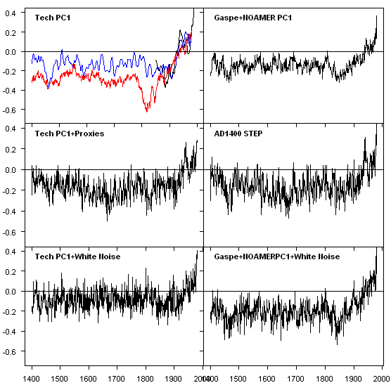
Figure 3. Left – Tech stocks; right – MBH. Top left – Tech PC1 (red), MBH recon (smoothed- blue). Top- Tech PC1 and Gaspé-NOAMER PC1 blend; Middle – plus network of actual proxies; Bottom – plus network of white noise.
I explained the experiments as follows:
To test the difference between MBH98 proxies and white noise, I tried the following experiments, illustrated in Figure 3 below (see explanation below the figure). I discuss RE results – the “preferred” metric for climatological reconstructions for each panel. As a benchmark, the RE statistic for the MBH98 AD1400 reconstruction (second right) is 0.46, said to be exceptionally significant.
Some time ago, I posted up the “Tech PC1”, which I obtained by replacing bristlecones with weekly tech stock prices, as an amusing illustration that Preisendorfer significance in a PC analysis did not prove that the PC was a temperature proxy. I re-cycled the Tech PC1 to compare its performance in climate reconstruction against that of the NOAMER PC1 (actually a blend of the NOAMER PC1 and Gaspé – the two “active ingredients” in the 15th century hockeystick.
In the top panels, I fitted both series against NH temperature in a 1902-1980 calibration period. The top right panel shows the Tech PC1 (red), together with MBH (smoothed- blue) and the CRU temperature (smoothed- black). The “Tech PC1″à actually a higher RE statistic (0.49) than the MBH98 reconstruction (0.46), but it does have a lower variance (in Huybers’ terms). The Tech PC1 has an RE of 0.49, slightly out-performing both the NOAMER PC1-Gaspé blend (RE: 0.46) and the MBH98 step itself (RE: 0.47). In the most simple-minded spurious significance terms, this should by itself evidence the possibility of spurious RE statistics. Both the Tech PC1 and the Gaspé-NOAMER blend have less variance than the target (and the MBH98 reconstruction itself.)
The second panesl show the effect of making up a proxy network with the other MBH98 proxies in the AD1400 network. In both cases, variance is added to the top panel series, in exactly the same way as in the examples with simulated PC1s. The RE for the Tech PC1 is lowered slightly (from 0.49 to 0.46) and remains virtually identical with the RE of the MBH98 reconstruction.
Now for some fun. The third panel shows the effect of using white noise in the network instead of actual MBH proxies. In each case, I did small simulations (100 iterations) to obtain RE distributions. For the “Tech PC1 reconstruction”, the median RE was 0.47 (99% – 0.59), while for the MBH98 case, using the NOAMER-Gaspé blend plus white noise proxies, the median RE was 0.48 (99% – 0.59). Thus, in a majority of runs, the RE statistic improves with the use of white noise instead of actual MBH98 proxies. The addition of variance using white noise is almost exactly identical to the addition of variance using actual MBH98 proxies.
The concluding comment was interesting and worth following up:
These results, which I find remarkable, tell me a lot about what is going on in the underlying structure of MBH98, which was, if you recall, a “novel” statistical methodology. Maybe the “novel” features should have been examined. (Of course, then they’d have had to say what they did.)
When I see the above figures, I am reminded of the following figure from Phillips [1998] , where Phillips observed that you can represent even smooth sine-generated curves by Wiener processes. The representation is not very efficient Phillips’ diagram required 125 Wiener terms to get the representation shown below.
Figure 4. Original Caption: The serieson
extended periodically.
Phillips’ Figure 2 is calculated using 1000 observations and 125 regressors. In the MBH98 regression-inversion step, the period being modeled is only 79 years, using 22 (!) different time series (a ratio of 4), increasing to use even more “proxies” in later periods. My suspicions right now is that the role of the “white noise proxies” in MBH98 works out as being equivalent to a “representation” of the NH temperature curve more or less like Figure 2 from Phillips. The role of the “active ingredients” is distinct and is more like a “classical” spurious regression. I find the combination to be pretty interesting.

Essentially what Mann did was to create a form of multivariate spurious regression. Traditional spurious regression – the type that you read about in Granger and Newbold 1974, Phillips 1986 – the type that econometricians are used to is univariate. Mannian spurious regression is a generalization of univariate spurious regression. You take one spurious regression (between Tech Stocks and NH temperature) between two unrelated trending series; and then insert this together with a large number of essentially white noise series (low-order red noise also works) in the Mannian multivariate method and bingo what have you got?
1) a high RE statistic
2) a negligible verification r2 statistic;
3) a high calibration r2 (and thus low standard errors in the calibration period)
4) seemingly narrow confidence intervals based on the low residuals in the calibration period.
It is, of course, a complete farce. The “no-PC” reconstruction bruited by Ammann and Wahl completely misunderstood the problems with the technique and carried it to an extreme that is almost a satire. Statistics by Monty Python, so to speak.


43 Comments
Steve, thanks for this post!
Can anyone explain me why the above described phenomenon (which IMHO is also appropriately called overfitting) seems to be so hard to understand to so many people (especially in relation to MBH)? Is it too technical, or is it simply that many otherwise skillful people want to believe in the results (talking about “denial”)?
On the lighter side, is there a method in John Langford’s Clever Methods of Overfitting-list that has not been (ab)used by the Team? 🙂
#1 – yes to both reasons. This also needs reduction in complexity to the the John Stossel “Give me a Break!” level of explanation (without it being totally sophomoric) for the statistically less-informed. I think most folks who get the gist of the argument just have a hard time solidifying the concepts behind it. Too many fuzzy areas and the brain gives up trying to put it together.
#1 – I like that list by John Langford! It’s almost like a team anthology.
Another way of looking at it, perhaps:
Steve: I notice that this chart points to the location of the Sheep Mountain bristlecones. Who knew?
Steve
May I respectfully request that your last sentence be used as the title of this article? I almost spewed my coffee reading that!
Note that MBH98 algorithm is robust in many ways, I changed the target (temperature to solar or number of nations), Steve changed responses (North A PC1 to tech stocks, others to white noise).
Steve — Please stop updating the bristlecone proxies. You’re going to cause the sun to go dim!
The trick would be to do a reconstruction with bogus series included. Then
when people ask for this mysterious series, you claim that it cannot be archived
because of “confidentiality agreements”
Once it passes peer review, you come clean with the fact that this bogus series
is the number of illegal aliens in the US.
You write the paper, I’ll put my name on it as the sole author. That way you pimp
the method and the peer review process in one fell swoop
Steve:
Could you, when you get a chance, look at the latest paper referenced by Rabett?
“A recent paper by Mathew Salzer and Malcolm Hughes in Quaternary Research 67 (2007) 5768 provides additional information. The paper has modest, but interesting goals.”
After RTFR, he zeros on one “point”:
“Looking at the tree ring index one can clearly see many large eruptions, the little ice age, but no European Warm Period, often called medieval.”
henry, that’s so old paper, Steve has already moved on 😉 Seriously, the paper was already noticed in CA in January:
http://www.climateaudit.org/?p=1094
Since Salzer&Hughes are finding “higher than expected correlation between Finnish pine and North American bristlecone”, I advice Eli to RWAFDAS (=”read what actually the Finnish dendro people are saying”). The web site is here:
http://lustiag.pp.fi/
Especially, see the latest poster Climate patterns in Northern Fennoscandia during the Last Millennium presented in the XVII INQUA Congress 2007. There is a nice bonus (a forecast!) in the bottom of the poster 😉
Sorry, hadn’t noticed that it was old, eli’s pushing it as “the newest thing”. It gave hiim a chance to push the “there’s no MWP here, move along…” story.
With permission, will adapt part of your reply to thread over there…
The question is, did Mann premedidate his selection of a generalization of univariate spurious regression? Did he begin with a specific outcome in mind? That is what inquiring minds want to know.
Was the malice aforethought, or only an afterthought?
==================================================
#12 — “The question is, did Mann premedidate his selection of a generalization of univariate spurious regression? Did he begin with a specific outcome in mind? That is what inquiring minds want to know.”
It doesn’t really matter, Steve. Mann is a trained physicist. Even if he was a bit negligent in his regression methods at first, he would quickly have figured out what he was doing well before he ever published anything.
[snip]
14, there were scientists who authored the SPM? I thought it was pretty much all NGOs and diplomatic types.
I’d like to see two series examined; world total mineral oil production and world synthetic surfactant. I bet they’d work if plugged in.
JF
I’d use the average weight of high school students and link global warming and obesity
(I thought I had posted this right before leaving for work, but apparently it didn’t make it…
To promote this, without getting nasty, perhaps one of the tech people would enjoy creating something like the Dilbert Mission Statement Generator but in this case, it would be a Hockey Stick generator. You could use the latest set of Google graphing tools to make it Very Cool.
Does anyone have access to other interesting data series that could help add to the quilt / matrix of graphs that demonstrate the amazing power of proxies to demonstrate AGW?
Some suggestions:
* Confirm the Nat’l Geographic “weighs the continents” theory: use Total number of National Geographic Magazines In Print as a proxy
* Use total # books in print
* Bring back the (divorce rate in UK?) classic example
Re #20
Some metrics come to mind, but I don’t know how many go back to 1900s…
1) Number of NGOs worldwide
2) Number of patents
3) Per annum presidential negative poll ratings
4) per annum presidential positive poll ratings
5) US Wheat Production ( see http://www.nass.usda.gov)
6) Ooh! Ooh! How about a hockey stick made of gold? Price of gold gives a nice double-bladed hockey stick.
It definitely would be fun to have a hockey stick generator! 🙂
Lovely..this is the best so far; it is plausable, uses established climate statistics methodology and demonstrates just how unprecedented… the recent rise in solar output has been.
Steve
I followed the link to Mann’s solar data and it is extremely interesting that he can reconstruct to three significant digits solar output based on proxy data when at the same time the acrim guys are pilloried for trying to fit overlapping measured data to two significant digits.
Re 10#, that forecast correlates with the 20th century US temperature record, and has us repeating the depths of the Little Ice Age from about 2035!
Chas,
That’s why they should update the proxies, and why divergence problem is an issue. Now we are in situation where temperature does not respond to sun from 1980 to present, but neither do proxies respond to 1980-present temperature (try to write this to RC and meet the delete button). One solution is to skip the temperature, tree rings respond to solar. But not with Mann’s MBH98 setup,
Ps. correct me if I’m wrong but: Doesn’t AR4 explicitly recognize they do practice
overfitting within climate models?. See page 596 section 8.1.3.1 of the tech. IPCC report (Pdf)
Click to access AR4WG1_Print_Ch08.pdf
best
Surely this whole thing is just “natural selection” in progress, a natural process. Proxies and statistics that fit, survive, others fall by the wayside.
We don’t need proxies, people, just like you and me, lived through this period, information on how and where they lived, what they grew, even what they wrote and illustrated is available. This will tell you more about climate change than any proxy.
Even the measurements can be interpreted to say whatever you want, or got wrong by mind numbing incompetence, as this site has pointed out.
Re; #10
Jean S,
Do you have a reference for the forecasting methodology for Figure 7?
Do you know how the tree rings were calibrated to temperature? Reference?
Thanks,
Mike
PS the Gleissberg Cycle jumps out of the smoothed data and the spectral analysis.
Re: 12, 14, 16
SteveM
Let’s try this again [my previous post was deleted].
Re: 14
Pat,
SteveS’ original question in #12 is very much to the point, indeed.
Your take on things ” he would quickly have figured out what he was doing well before he published anything” in fact contains the answer to the question. To publish something you know is false/incorrect/biased, etc., and stick handle it through “peer review” is a deliberate act, and is best described by the very terminology that our host does not wish to see on this blog [his perogative].
Re: 16
In the business world SteveS’ opening contention would be correct. Based on all available evidence in the Mann case, academe doesn’t seem to see it that way.
Steve,
I’m certain I have no idea what multivariate spurious regression is but I think I get the gist of this. Do you get hockey sticks with all series you try or could a series be fabricated that would not result in the hockey stick?
It’s more that there are a lot of unrelated series that you can find that will generate seemingly significant reconstructions – that’s what happens with “spurious regression” e.g. the classic relationship between Church of England marriages and alcoholism rates reported by Yule in 1927. Those were univariate spurious regressions.
In Yule’s example, Mann’s system would be more like attempting a proxy reconstruction UK alcoholism rates in which the predictors were Church of England marriages and 20 series of white noise (or noise like things like Morocco tree rings). In a Mannian reconstruction, you would get an alcoholism reconstruction with a high RE statistic. Different terminology but the same old spurious regression.
If you wanted a reconstruction of alcoholism in the England in the 15th century, I’m sure that bristlecones would give a model with an excellent RE statistic. Tihis would be along the lines of UC’s solar reconstruction or number of nations or any number of other amusing examples.
#26: Mike, unfortunately I do not know. I suppose you have to wait (or try e-mailing the authors if you’re in rush) for the paper referenced in the poster to be published.
Reading the poster I think the forecasting method is something simple like representing the index by the dominant Fourier series terms. The thing that makes the forecast IMO somewhat newsworthy is the length of the index (something like 7500 years). In other words, IF the model is of any good, it is likely estimated correctly and the forecast might be reasonable.
Yes, the correspondence to the solar cycles was something that came to my mind also.
#30 Jean S
I expect you are right about the Fourier forecasting, and as you say, the length of the data series gives credibility so long as the pattern is stable and consistent.
It would be interesting if they did C14 analysis of the wood to see if the solar ray variation matches the ring width variation. See Karlen and Kulenstierna did C14 analysis of pines above current tree line in Scandinavia The Holocene 6,3 (1996)pp 35 9-365 revealing a solar signal.
The forecast matches the ones based on forecasts of solar cycles 24 and 25, which will be much less active, perhaps as low as the Maunder Minimum, particularly 25 (there is disagreement over how much less 24 will be. Just google solar cycle 24 25 and you will find forecasts from NOAA, NASA and others.
See also the Archibald presentation posted in July at Warwick Hughes’blog.
Thanks to Jean S bringing our INQUA poster and a very important question into the forum. But one correction first: the Helama et al. paper does not include the forecast model; it will be published in another paper still in process and the author of this message (Mauri Timonen) responsible for that.
Please, dont count too much on the tentative forecast model that even has no confidence limits! It was meant for a poster discussion only and is subject to change as I and some of my colleagues continue the model development. We hope to introduce a working forecast of natural climate variation in northern Finland for the next 100 years.
I personally was earlier a bit shy to model climate periodicity, because there is almost always a problem to find a good explanation for the observed cycles. But now, having got much more familiar with the characteristics of our supralong climate sensitive, 7641 years long Scots pine chronology, I am much more convinced that there must be some specific cycles. The 80 95-yr cycle indeed seems to push through in different connections, not only in tree-rings. I got to know from my Finnish colleagues in geology that their 12000 years long lake sediment chronology also signals this cycle. Maybe the Gleissberg cycle has even a greater importance than by now believed!
As looking carefully at the FFT filtered tree-ring index cycles of the poster, some regular patterns can be identified both in the tree-ring index amplitudes and in the cycle lengths. The problem, however, is that the cycles tend to change by time. This makes forecasting based on long periods (>1000 years) puzzled. In the case of the discussed tentative model, it is actually based on the last 500 years(!) The cycles of this period are, like Mike says, enough stable for simple forecasting. If the regularity of the last five cycles continues (we of course have to filter out some disturbing factors like the active volcanic activity in the 1800s), there exists a very nice sine type cyclicity. If this rhythm continues, we are very strong to forecast the natural future climate! If not, then we just can spread our hands and explain: climates basic nature is just chaotic: we are switching from one stage to another… Thats the normal story in our chaotic climate, over history.
Anyway, we shall finish our forecast model, which might be working even splendidly in a stable condition. But as said before: it is as good as the previous stage of climate
If forecasting of natural climate variation based on tree-rings really works also after model verification + monitoring and climate also keeps stable, we are closer to answer the question, which role natural variation plays in our (Finnish) climate system.
– – –
By the way, our tree-ring data will be available at the latest by 2010, as we introduce our Finnish Tree-Ring data-metadatabase in the WorldDendro2010 meeting in Rovaniemi; check at http://lustiag.pp.fi/wd2010.htm.
Best Wishes, Mauri
For direct contacts:
Mauri Timonen +358 10211 4472
mauri.timonen@metla.fi
And: Do not forget to check the many topics of http://www.lustia.fi !!!
Mauri, thank you for a valuable comment and welcome to ClimateAudit!
I don’t know if you have tried, but there exist some methods which might be more appropriate to your situation than the classical Fourier analysis, see time-frequency analysis.
Can you point to a paper (to answer Mike’s question in #26) explaining how you calibrated the index to the temperature? What standardization method you used for the index? I somehow recall that you are not using the standard RCS, but you have developed an improved method (I might be completely wrong about this).
Mauri.
I love the site and the approach! Maybe SteveMc should link your site!
Re: 10,26,30,31,33,34
Jean S and Steven: Thanks for advising and encouraging me!
Here some references you requested:
About our RCS techniques (developed by Samuli Helama):
Helama, S., Timonen, M., Lindholm, M., Meriläinen, J. & Eronen, M. 2005. Extracting long-period climate fluctuations from tree-ring chronologies over timescales of centuries to millennia. International Journal of Climatology 25 (13): 1767-1779.
About our techniques to calibrate the index to the temperature:
Helama, S., Lindholm, M., Timonen, M., Eronen, M. & Meriläinen, J. 2002. Part 2: Interannual-to-centennial variability in summer temperatures in northern Fennoscandia during the last 7500 years extracted from tree-rings of Scots pine. The Holocene 12(6): 681-687
About building the supralong Scots pine chronology:
Eronen, M., Zetterberg, P., Briffa, K., Lindholm, M., Meriläinen, J. & Timonen M. 2002. Part 1: The supra-long Scots pine tree-ring record for northern Finnish Lapland; Chronology construction and initial inferences. The Holocene 12(6): 673-680.
Methodology Page:
We use several statistical approaches in our tree-ring chronology and climate constructions. Because of continuous interest in our Finnish tree-ring studies, I have decided to establish a separate theme page called Methodology Page on the Lustia website for describing our way of working with tree-rings. This concerns also the sampling techniques and the sample sizes that play an emphasized role in the case of tree-ring width analyses. Compared to ring width data sampling, isotope and density data sampling, for example, are much more consistent. Making comparisons with different proxies and trying to expose the best proxy variable as terms of the strongest climate signal, is not a very good idea for this reason. Generally, all proxies are important, because they tell about different aspects of climate.
Cheerleading from the peanut gallery… welcome from a fellow Finn! (I’m half Finnish — Wainionpaa 🙂 )
#35
Mauri,
Interesting article, short question: how did you calculate 95 % confidence limits in Figure 1 middle plot? Clearly something different than 2X sample std of calibration residuals.
“Tech PC1″, which I obtained by replacing bristlecones with weekly tech stock prices”
Reverse the chronological order of the stock prices and try again. It is possible that stock prices have tended to go up recently; see if the reversed order still produces a graph with a recent climb.
Re # 18 MrPete
An old one but a good one:
Storks Deliver Babies (p = 0.008) Robert Matthews
There is a highly statistically significant correlation between stork populations and human birth rates across Europe. While storks may not deliver babies, unthinking interpretation of correlation and p-values can certainly deliver unreliable conclusions.
Re $ 29 Steve
Univariate regression, C of E marriages and alcoholism. Possibly not.
The river waters of England were so polluted for centuries that death was a common result from drinking water. You cannot marry too easily when dead, though some wives accuse husbands of a similar state. The cure was firstly to add alcohol, which killed a number of bugs. Sci-Am once had an article which concluded that for some centuries the usual condition of the European populace was “inebriated”, even down to small children. It had population estimates of alcoholism.
Matters improved a bit when tea came from China before 1800, because boiling the water also killed nasties and tea left a clearer mind than alcohol. Next development was chlorination of public water supplies, which started in London in 1903. We presume that this also caused a lower reliance on grog, but then one has to make a Skill Judgement based on Experience and Undoubted Intelligence and Excellence in Chosen Field of Knowledge.
The question is, with fewer people sozzled, would this lead to more marriages (through people of marriage age being more prevalent and more presentable) or fewer marriages (because sober people might think twice before tying the knot). So, the marriage rate was not a constant – it was perturbed by known secondary effects, calling for multivariate stats.
The interesting question is why the Church of England was selected for the stats comparison, and not another Church. One can predict that the Methodist Church would have a systematic bias, as Methodists did not make love standing up. (Reason? It might encourage them to dance). The Catholic Church was over-represented by people of Irish descent and as a group they drank so much that they would not accurately recall or record if they were married or not, once or more, in sequence or simultaneously.
The closest answer I can give to the Choice of C of E was that they were sexy little devils, with the males well into the art of cherry picking before, during or after marriage.
See, nothing is really very simple in stats.
UC #35 November 4th, 2007: Interesting article, short question: how did you calculate 95 % confidence limits in Figure 1 middle plot? Clearly something different than 2X sample std of calibration residuals
Shamed for my over three-week delayed reply! But I, unfortinately, have not, during this period, had a possibility to recalculate our seven-year old data. But it still seems to me that the confidence limits are most probably properly calculated. But we used a simple tree-ring index to temperature conversion to create the modelled average temperature data. Deriving the confidence limits based on this approach, give more accurate results with more replications and vice versa. But if you have any better ideas how to deal with tree-ring based temperature estimate confidence limits, just let us know: we try to recalculate our old data based on your instructions – and also our new one, about 1.5 more replicated data! And if you also would like to try with our data, just let us know and we are ready to consider to cooperate! Cheers, Mauri
Cheers, Mauri!
UC #35 November 4th, 2007: Interesting article, short question: how did you calculate 95 % confidence limits in Figure 1 middle plot? Clearly something different than 2X sample std of calibration residuals
Sorry again for my learning to use this forum! My message was supposed to sound something like this:
Shamed for my over three-week delayed reply! But I, unfortinately, have not, during this period, had a possibility to recalculate our seven-year old data. It still seems to me that the confidence limits are most probably properly calculated. We used a simple tree-ring index to temperature conversion to create the modelled average temperature data. Deriving the confidence limits based on this approach, give more accurate results with more replications and vice versa. If you have any better ideas how to deal with tree-ring based temperature estimate confidence limits, just let us know: we try to recalculate our old data based on your instructions – and also our new one, about 1.5 more replicated data! And if you also would like to try with our data, just let us know, and we are ready to consider to cooperate!
Cheers, Mauri!
Mauri,
No worries, I just read your reply (remembered this because of discussion in more recent thread, http://www.climateaudit.org/?p=3348 ) 😉 .
I have some ideas, but first I’d like to see a reference where the conventional method is described thoroughly.
3 Trackbacks
[…] networks constructed to emulate the MBH98 network (Huybers #2 and Reply to Huybers) also here and I’ll try to tie these three different studies […]
[…] of white noise, you can achieve arbitrarily high correlations. (See an early CA post on this here discussing example from Phillips […]
[…] of white noise, you can achieve arbitrarily high correlations. (See an early CA post on this here discussing example from Phillips […]