We’ve all had enough experience with the merry adjusters to know that just because someone “adjusts” something doesn’t necessarily mean that the adjustment makes sense. A lot of the time, the adjuster arm waves through the documentation and justification of the adjustment. Today I’m going to work through aspects of one of the most problematic adjustments in this field: the MBH99 adjustment for CO2 fertilization – something that some of us have wondered about for a couple of years. In this particular case, there are a number of crossword puzzles and I’d welcome solutions to these puzzles, as I’ve pondered most of these issues for a long time and remain stumped. I’m not discussing here whether CO2 fertilization exists or not, but merely whether the Mannian approach is a reasonable approach to the issue, trying first merely to understand what the approach is.
I’m working towards assessing the impact of the new Abaneh Sheep Mountain data on the Mannian-style results – and the impact on the Mann and Jones 2003 PC1 (used by Osborn and Briffa 2006; IPCC AR4; etc.)
The MBH99 adjustment is explained as follows (and this discussion immediately precedes the log CO2 argument that I just posted on):
A number of the highest elevation chronologies in the western U.S. do appear, however, to have exhibited long-term growth increases that are more dramatic than can be explained by instrumental temperature trends in these regions. Graybill and Idso [1993] suggest that such high-elevation, CO2-limited trees, in moisture-stressed environments, should exhibit a growth response to increasing CO2 levels. Though ITRDB PC #1 shows signfi cant loadings among many of the 28 constituent series, the largest are indeed found on high-elevation western U.S. sites. The ITRDB PC#1 is shown along with that of the composite NT series, during their 1400-1980 period of overlap (Figure 1a). The low-frequency coherence of the ITRDB PC#1 series and composite NT series during the initial four centuries of overlap (1400-1800) is fairly remarkable, considering that the two series record variations in entirely different environments and regions. In the 19th century, however, the series diverge. As there is no a priori reason to expect the CO2 effect discussed above to apply to the NT series, and, furthermore, that series has been verified through cross-comparison with a variety of proxy series in nearby regions [Overpeck et al, 1997], it is plausible that the divergence of the two series, is related to a CO2 influence on the ITRDB PC #1 series.
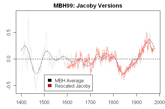
There are obviously other possible approaches to adjusting for CO2 fertilization if one is worried about that. One possible method would be to do a correlation of the growth pulse to CO2 and work with the residuals. This would be an approach consistent with age detrending methods in dendrochronology and you’d think that Mann might have tried something like this. (I’ll discuss this on another occasion.) Here is the Figure 1a from MBH99 showing the “target” Jacoby series, the PC1 in need of adjustment and the adjusted PC1.
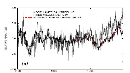
MBH99 Figure 1a. Comparison of ITRDB PC#1 and NT series. (a) composite NT series vs. ITRDB PC #1 series during AD 1400-1980 overlap. Thick curves indicate smoothed (75 year low-passed) versions of the series. The smoothed “corrected” ITRDB PC #1 series (see below) is shown for comparison.
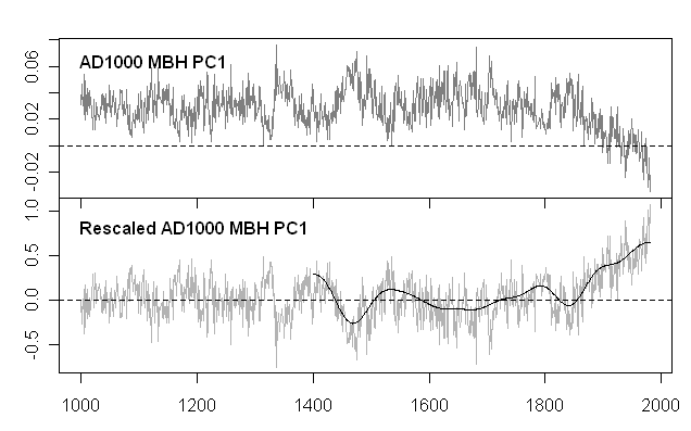
The above graphic is pretty muddy. Here is a re-drafting of the graphic to show the features a little more clearly. In making this graphic, I’ve used data versions stored at the former Virginia Mann FTP site. In the directory TREE/COMPARE, it contains nearly 100 versions of different series, which I visit from time to time to try to decode. I’ve made a little push recently (and thus the post before I forget.) The light blue series is a plot of a rescaled version of the AD1000 Mannomatic PC1 (together with a smooth); the grey series is a plot of an average of Jacoby chronologies (together with a smooth) and the red dashed line is the adjusted PC1 (in a smooth version). I can sort of mock up the rescaling of the PC1 but the rescaling principles remain a mystery as discussed below.
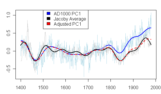
Figure 2. Re-drafting of MBH99 Figure 1a.
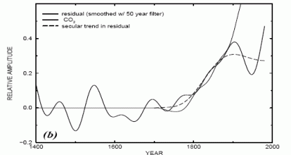
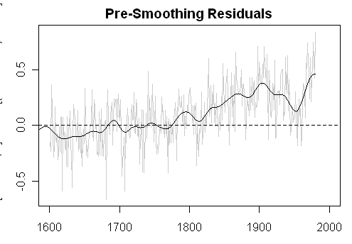
Continuing a quick overview of the adjustment before looking at the details, Mann deducts the smoothed Jacoby average from the smoothed Mannomatic PC1 to get a “residual”, shown in MBH98 Figure 1b (left panel below). He then carries out another smoothing operation on these already smoothed residuals to get a “secular trend” – which he compares to CO2 increases (already discussed.) This “secular trend” is then backed out of the Mannomatic PC1 to get what Mann calls a “fixed” PC1 – although I think that the term “adjusted” is more apt. In the right panel, as a short exercise, I’ve done a similar comparison between the incorrectly Mannomatic PC1 and the AD1000 correlation PC1. The AD1000 network is already heavily dominated by bristlecones, so the difference between the correlation PC1 (or covariance PC1) and the Mannomatic PC1 isn’t large for this network – an observation that we made in MM2005 (EE). (The difference is large for the AD1400 network, as has been endlessly discussed.) What’s intriguing here is that the “adjustment” required to reduce the Mannomatic PC1 to the correlation PC1 is almost exactly the same amount as the vaunted “CO2 adjustment” although it gets implemented in the 20th century rather than the 19th century.
 |
 |
The Jacoby “Target”
The most obvious question in this exercise is: why is the Jacoby series selected as a “target” against which to adjust for CO2 fertilization? If there were regional differences between California and northern Canada in the timing of emergence from the Little Ice Age, then spurious correlations might easily arise between low-frequency series. Wouldn’t it make more sense to use something like the Briffa et al 1992 temperature reconstruction (a reconstruction referred to in the Ababneh thesis)? What would be the impact of using some other target? I doubt that I’ll get to some of these analyses as the data from the Ababneh thesis is going to make some of these speculations very moot. From a statistical point of view, in assessing “confidence” for these calculations, it’s just that one has to remember that the Jacoby target has been selected from a larger population and was not selected randomly.
Next, there are some differences between the Jacoby target used in MBH99 and the reconstruction published by Jacoby and D’Arrigo (1989, 1992). The MBH Jacoby version goes 200 years earlier than the Jacoby-d’Arrigo reconstruction, which began only in 1601, not in 1400.) The figure below compares the Jacoby and d’Arrigo reconstruction (scaled to match the MBH99 version) and the MBH99 target (light grey).
Next, the Jacoby chronologies used in MBH99 were obsolete even at the time – a point made in MM03. For example, Mann used a TTHH chronology with values back to 1459 while the archived chronology goes back only to 1530. In the final archive, no chronology is presented for a period that does not contain at least 3 cores: Mann used an early version which included a period prior to 1513 where there was only one core. In MBH, Mann stated that they carried out quality control on their chronologies to ensure that there was a match between the measurement data and the chronology. In the case of one of the Jacoby chronologies (Churchill), there was negligible correlation according to this test. A couple of years ago, I wrote to Rosanne D’Arrigo observing that the Churchill chronology could not obtained from the archived measurement data. She said that the archived chronology was wrong and said that she would replace it at ITRDB; however, this has not taken place two years later.
In the 15th century portion of the Mann version, a very old Coppermine chronology is used (values from 1428-1977). I inspected the measurement data and determined that this data set only had one tree (two cores) with values prior to 1500. This portion of the chronology does not meet normal QC standards for the minimum number of trees to form a chronology (including standards said to have been applied in MBH – a minimum of 5). The only Jacoby chronology contributing to the earliest part of the 15th century is Gaspé – about which much has been said in the past. In the earliest portion of the Gaspé chronology, there is only one tree.
A more fundamental problem with the 11 Jacoby chronologies is the risk that the selection has been contaminated by cherrypicking. At the NAS Panel, D’Arrigo told an astonished panel: you have to pick cherries if you want to make cherry pie. In Jacoby and D’Arrigo 1989, they reported that they used (and archived) only the 10 most “temperature sensitive” treeline series (to which they added Gaspé known to have a pronounced HS shape.) If you take a network of 36 red noise series with relatively high autocorrelations (as Jacoby chronologies) and pick and average the 10 with the biggest 20th century trends, you’ll get something that looks like the Jacoby average. A proper evaluation of the statistical significance of “adjusting” the Mannomatic PC1 to such a target is needless to say not discussed in the underlying literature.
The Divergence Problem is also an issue. One of the series in the target Jacoby average is Twisted Tree Heartrot Hill (TTHH), which has been recently updated (but not archived). Davi et al (including D’Arrigo) observed a Divergence Problem at this site (see Jacoby category -scroll back).
In replication terms, it is possible to arithmetically calculate the MBH version of the Jacoby average and, in this case, the chronologies as used and the average were all digitally available at one point. The issues here pertain primarily to the significance and selection of the target for the coercion.
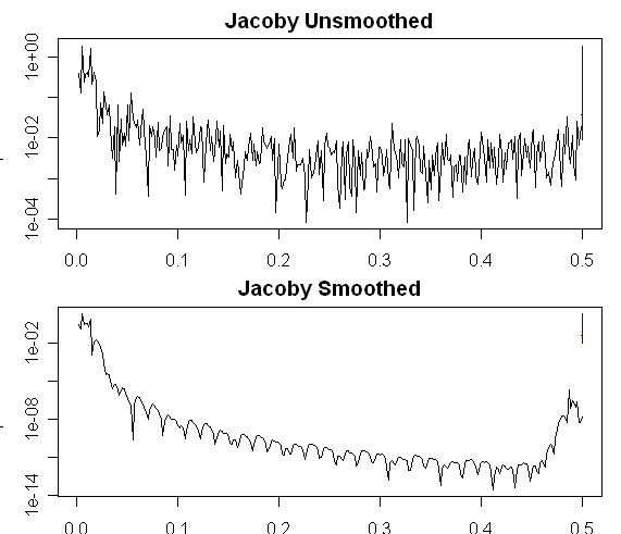
Smoothing the Jacoby Average
Now, a little Mannian puzzle. How is the smooth of the Jacoby average done? In this case, we have the input data and the output data, so it’s possible to see if we can match the result. In the caption to Figure 1b, Mann says that you used a “75 year low-passed” filter. In tree ring jargon, a “75 year” filter is often used to describe a filter with gaussian weights that is long enough to pass 50% of the variance through 75 years (see Meko’s notes on this). In the figure below, I tried a 75-year gaussian filter and get something that looks similar to the Mannian result, but not the same. I’ve experiment with other filters and other end period approaches – reflection padding and Mannomatic padding yield worse results. Lowess filters don’t improve things. So I don’t know. I’ve archived materials for people to test: see columns 1 and 2 in the data set. A smoothing point to bear in mind: why is the delta calculated after smoothing: does it matter if the deltas are calculated first and smoothing done later?
I also checked circular padding in the smooth – it was a little improved but didn’t resolve the problem.
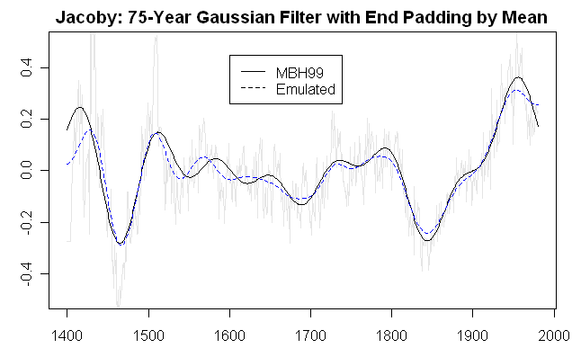
Figure . MBH Jacoby average: MBH smooth and smooth with 75-year gaussian filter with mean padding.
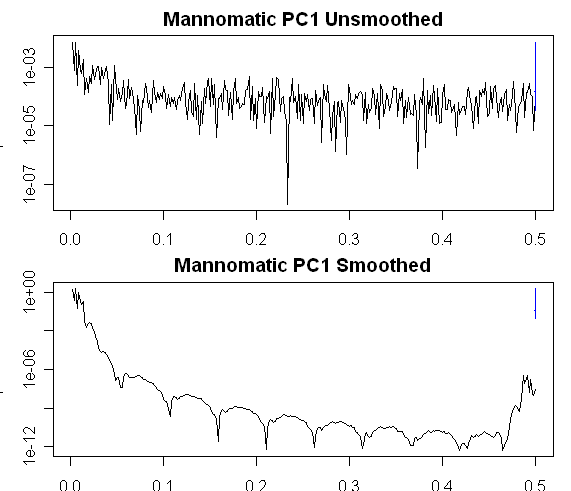
Smoothing the Rescaled Mannomatic PC1
There’s a tricky re-scaling step in the PC1 illustration, which is the next step in the logic, but before discussing it, I’m going to discuss the smoothing step for the Mannomatic PC1, just in case this helps decode the smoothing methods. Here the calculation starts with the Mannomatic PC1 (known to be “incorrectly” calculated – not that I believe that “correctly” calculated PC1 necessarily means anything.) Once again, I’ve tried a 75-year gaussian smooth and find that it is related to the archived version, but isn’t quite the same. I’ve provided materials (cols 3-4) for puzzle solvers.
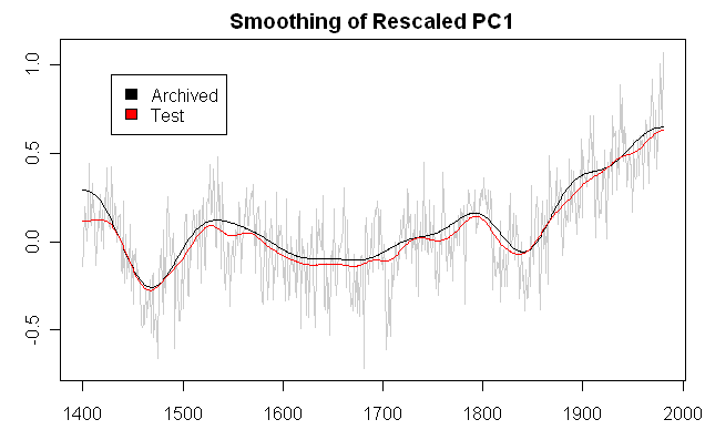
Figure. Smoothing the Mannomatic AD1000 PC1. Only the 1400-1980 period is shown.
While we’re thinking about Mannian smoothing, I’ll jump out of sequence and discuss smoothing of the “residuals” to yield a secular trend as discussed above. The legend to MBH99 Figure 1b says that the residuals have been smoothed with a 50-year filter (even though the two predecessor series had already been constructed with 75 year smooths.) The caption to MBH99 Figure 1b (perhaps inconsistently) says that the “secular trend” was calculated “retaining timescales longer than 150 years”. How was this smooth actually calculated? I don’t know. I’ve been able to replicate this result more closely than the other smooths by using a lowess smooth with f=0.3. I doubt that this is what Mann did. As noted previously, there is a big difference in interpretation between Mann’s conclusion that the supposed effect has “leveled” off in the 20th century based on one smooth and the continuing upward trend in the first smooth. Something else that some readers might wish to consider: is it possible that we’re a seeing some Slutsky effect here. (For non-econometricians, the Slutsky effect is a classic and elegant proof from the 1930s that repeated smoothing/averaging operations on time series will push them towards a sine curve.)
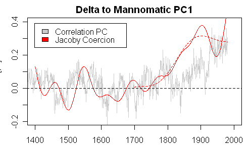
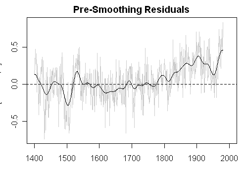
I’ve plotted the actual differences between the two series below (for whatever that’s worth) together with a 50-year smooth. I wouldn’t characterize this plot as showing a discrepancy arising in the 19th century and then leveling off in the 20th century. On the right, I’ve limited the plot to the period of the actual Jacoby-D’Arrigo chronology 1601-1980, to minimize the rhetorical effect of the 15th century where there are only 1-2 trees involved. In this case, one would surely characterize the plots not as showing remarkable similarity prior to 1800, but as the bristlecone PC1 gaining relative to the Jacoby reconstruction, with the relative gain reversed only during the HS-pulse of the Jacoby series in the early 20th century.
 |
 |
Re-scaling the AD1000 PC1
Now for a tricky part, that’s annoyed me greatly. In the log CO2 diagram, I’ve showed the mysterious appearance of arbitrary re-scaling with no explanation for what seems to be no more than rhetorical purposes.
In the top panel, I’ve shown the Mannian AD1000 PC1 as originally calculated. I can replicate this calculation from original chronologies (using the incorrect Mannian PC method.) The plot here is from the PC1 at the former Virginia Mann FTP site. It is inverted. PC series have no native orientation and the inversion here doesn’t trouble me. If you want to interpret the PC1 as a weighted average of the underlying chronologies (mostly bristlecones), then you can choose the orientation from positive weights as opposed to negative weights. A second point about the native series is that the PC series is calculated here from an svd algorithm and as a result the sum of squares adds to 1 i.e. the amplitude is very small. Occasionally one sees internet commentary purporting to find a flaw in the red noise simulations in MM (2005 GRL) on the basis that the amplitude of the PC series is “too small”; the amplitude of our simulations is exactly the same as the amplitude of the Mannian PC1 and the people who raise this argument don’t know what they’re talking about (not that that stops them.)
Aside from the inversion of the series, one can see both a rescaling and a recentering, which is not described and I’ve not been able to figure out at all. Another crossword puzzle.
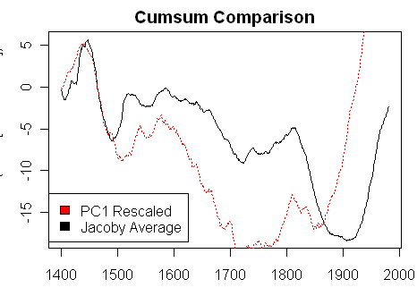
It looks as though the rescaled PC1 has been recentered on some portion of 1400-1900 so that it more or less matches the mean of the “target” Jacoby series in the 1400-1780? period. We’ve seen from the log CO2 diagram that these selections can be opportunistic. If the Jacoby series has been used as a target reference, then it should be possible to find some period over which the Rescaled PC1 mean is equal to the Jacoby mean. As a way of exploring for such a period, I plotted cusums for the rescaled PC1 and the Jacoby target as shown below: they cross for a period of about 1400-1865. Or maybe the reference period doesn’t start in 1400 but some other period. It’s hard to say. But it looks like something like this is going on. Of course, this sort of calculation presumes mathematical precision. Ideas are welcome.
A tougher problem occurs with the rescaling of the PC1. The sd of the PC1 (0.21) is higher over (say) the 1400-1865 period .than the sd of the Jacoby average (0.18). You can see this in the diagrams. So it’s not obvious how the PC1 has been rescaled. Is there some period over which the sd of the target matches the sd of the rescaled PC1? To test this, I did a “cumsd” calculation modeled on the cusum calculation for means. In this case, the two standard deviations match for a reference period of 1400-1600, which is round, but do not match for other periods. Did Mann re-center and re-scale on different periods? If so why? Or is there some other rescaling principle entirely? I have no idea how this rescaling was done and it bugs me.
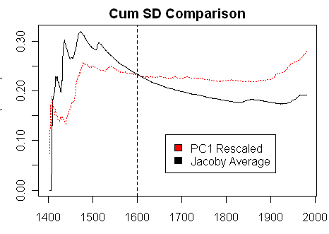
Black: Cumsd Jacoby NH; red – cumsd – pc1-rescaled. Looks like a round match at 1400-1600.
Data
I’ve collated the following series into a data file in case anyone can solve any of the smoothing or rescaling problems:
1- Year
2 – Jacoby average, unsmoothed
3 – Jacoby average – Mannian smooth
4 – Mannomatic PC1 – native unsmoothed
5 – Mannomatic PC1 – rescaled unsmoothed
6 – Mannomatic PC1 – smoothed 1400-1980
7 – Mannomatic PC1 – adjusted
8 – Smooth residuals
9 – Secular trend
7 – Mann CO2
8 – Mann log CO2 ratio
Aside from solving the various crossword puzzles, the more fundamental issue is: is this a valid way of adjusting the Mannian PC1? Does it make any sense to try to adjust the PC1 (as opposed to the individual chronologies)? What if the growth pulse in the bristlecones was not related to CO2 fertilization – an effect denied by other writers in the field?
In a subsequent post, I’m going to show the impact of the Ababneh Sheep Mountain chronology on the Mann and Jones 2003 PC1: it’s very dramatic raising some serious questions about exactly what, if anything, is accomplished in these Mannian adjustments.
UPDATE: Here are spectra showing impact of smoothings:


67 Comments
Given previous discussion about what exactly a PC is I would think that “adjusting” one makes little sense. See, the step of adjusting is based on the proposition that a precisely identifiable component of the PC is related to whatever one is adjusting for. But PCs are just orthogonal vectors chosen to fit a particular mathematical objective. PC1 is not a “temperature” component or a “CO2” component – it’s just the component that explains the most variation in the data. If you are going to adjust, you should at least do it rigorously with some sort of regression – and if you have omitted variables bias in a regression of PC1 on CO2 the result will be a mess. Perhaps, if one was trying for internal consistency, the “adjustment” should be to regress PC1 on CO2 and local temerature and whatever else might be relevant and then remove the CO2 component. But that papers over a multitude of sins.
But, assuming for the moment that we still want to go down the PC track, let’s think about the problem. We would like a PC series that is “orthogonal” to the CO2 signal. It would seem to make more sense to remove the CO2 signal prior to compiling the PCs than after. So, if you want to remove the CO2 signal you should, say, regress all your individual series on the CO2 series and then use the residuals to construct the PCs. This will ensure that all your PCs are orthogonal to the CO2 series. (There are ubdoubtedly more elegant and more efficient ways of doing this. I imagine that you could generate orthogonality to the CO2 series by some careful work in the PC generation step by choosing an appropriate rotation.) This will also “ensure” that there is no CO2 signal in other PCs.
So, to answer your question I think that adjustment of individual chronologies makes more sense (in this Bizzaro world where any of this makes sense). I also think that “adjustment” of a PC after the fact imposes a physical interpretation on what exactly the PC is – and that interpretation needs justification that seems to be somewhat lacking in this case.
Two quick points off the top of the head:
1. Fertilisation of vegetation changes yield in complex ways. Roughly, there are some 20 nutrient elements including hydrogen as pH, plus organic compounds like auxins, plus organisms like bacteria, etc that can interact. Most, if not all of these, do not act alone and in a linear manner. Some are monotonic, others have U shaped response, but the response changes as other nutrients change. One needs to do analysis of variance using several levels of each nutrient to merely start on an understanding. There is no magic basis that says that a change in CO2 alone will lead to growth in a certain manner that can be predicted without actual experiment.
2. There might be studies that show that tree rings change character with more/less of certain fertilisation regimes, but I have not seen any. (I’m rusty). It might be logical to infer that tree rings change in certain ways, but proof not inference is needed in each case. At least, that’s my understanding of rigour in Science.
Re: filtering
I bet they used ITRDB’s ARSTAN.
As in #3.
I bet Mann did not do the smoothing himself, but had some dendro do it for him, therefore he couldn’t accurately describe the process himself. ARSTAN is an arcane DOS-based program that is fairly opaque and does not even run on modern computers. You would have a tough time replicating what it does using LOWESS.
I don’t ask this question lightly: Is there a possibility that direct, post-processing manual modification of the output data sets has been performed?
If someone is up to the challenge, ARSTAN is available for Windows XP here
#6: Works as advertised!
FYI: I asked Dr. Mann directly about this adjustment at RC. Here’s how it went: http://www.realclimate.org/index.php?p=253#comment-8567
#4. Mann is big on smoothing. He did the smoothing himself.
BTW a few years ago, I did quite a bot of experimenting with ARSTAN. I was able to accurately replicate ARSTAN coefficients using the nls function in R and I have some R functions that do tree ring chronologies quite well. I haven’t done all the diagnostics but I could. There are some interesting numerical issues of a Bruce McCullough type. The math is pretty trivial in R.
I recall one intriguing error in the ARSTAN routine. If there were 20 cores, it always calculated the coefficients of the 1st core wrong, although the other ones were calculated OK. You can get somewhat different answers as well if you modify the number of iterations to reach convergence.
I’ll post up my emulator some time. I did this pre-blog.
Apologies for the temporary brain cramp, but ARSTAN is used for detrending, not smoothing. Doh. Too many late nights.
Re: the recentering and scaling step. Did he do this manually himself, or were these options chosen as part of the PC/SVD routine?
Steve: This has nothing to do with Mannian PCs.
Re: 5
Scott-in-WA
I would second that question, equally carefully. Suggestions, anyone?
#5. I know of one case where we firmly established manual post-processing of the data. Mann manually extended the Gaspe tree ring series from 1404 to 1400. The purpose of this extrapolation was to add the Gaspe series (with a big HS) to the AD1400 calculation step (which tends to run a bit warm with Mann’s proxies.) This is the only such extrapolation in the entire Mann corpus and was not reported.
Another manual change is discussed here:
Their processes for deleting sites from the various networks remains a mystery. They deleted a large number of Brubaker-Graumlich sites in Washington which seem as good or as bad as any other sites. Their explanation of the unreported deletions in the Corrigendum was false; I advised NAture of this prior to publication of the Corrigendum, but Nature didn’t care whether the explanation was correct or not.
Re # 8 nanny_govt_sucks
Looked up the rc link and a few posts down (on the subject of CO2 fertilisation) found
This for me was the last word from a discredited armwaver. Steve, when can this rubbish be acted upon through formal circles? It is taking up a lot of your time (and mine, I’m fascinated by your forensic skill) but there has to be an end point where there is a public admission and correction.
BTW, my first stats in 1964 were manual ANOV on plant nutrition experiments using Fisher’s method, pre-computers. I’ve forgotton a lot since, but can follow these threads but not be original. My apologies for being a generalist. It seems like a lot of the fundamental physics taught at the time, like Stefan-Botlzmann, Wein’s displacement, etc, need to be retaught to whizz kids.
RE: NO. 8 – nanny_govt asks Dr. Mann about adjustment for CO2 fertilization
“The vast scientific literature on this sort of stuff” can be located at:
http://www.co2science.org/scripts/CO2ScienceB2C/data/plant_growth/dry/dry_subject.jsp
The following recent paper may help assess Dr. Mann’s statement concerning stomatal evapotranspiration limitations:
Photosynthetic and Stomatal Conductance Responses of Plants to Atmospheric CO2 Enrichment by Ainsworth, E.A. and Rogers, A. 2007
Click to access Ainsworth_&_Rogers_2007.pdf
Take first difference of the adjustment,
diff(mannpc1_adj-mannpc1_resc)
and you’ll see that the adjustment is composed of 7 lines, exactly. See Jean’s comment,
Re # 15 Webster Hubble Telescope
Care to read the whole paper?
The Annals of Statistics 1984, 12, 2,pp 665-674
“On the Sinusoidal Limits of Stationary Time Series”
Kedem, Benjamin.
Part of introduction:
“In the Gaussian case, as we shall see, the Sinusoidal Limit Theory (SLT) of Slutsky is a natural consequence of relations between conspicuous visual features depicted by time series graphs…..”
Sure, this is a bit qualified, but it does not demand the response that you gave. I am a nice person, a scientist in the real world with an interest in the integrity of science. Can I ask you to please write with civility.
RE Mann’s response
“Response: Actually, not. It is well understood by those who study terrestrial ecosystem dynamics that there are multiple limiting factors on growth. For example, once a tree has essentially as much CO2 as it can use, other conditions such as soil nitrogen availability, will become limiting. In addition, the longer the stomates remain open (to try to take in the additional CO2), the more vulnerable the tree becomes to water loss through evapotranspiration. So one would only expect a significant impact of Co2 fertilization only until these other limiting factors kick in. Any subsequent increase in ambient CO2 concentrations would have little incremental value to the tree once this happens. A plateau in the observed response is the rule, not the exception. There is a vast scientific literature on this sort of stuff. Well leave it at that. – mike]”
What utter drivel- the main point being that elevated CO2 rsults in stomatal closure- which, in turn, raise water use efficiency.
The Mann is either ignorant, a liar, or both.
More iluminating stuff from RC–
“With all of these results graphed together, it is a little hard to read. However, several things I note:
1) Excluding the instrument data (which we cant use to compare to 1000 years of data, anyway) it is apparent that we have seen temperatures comparable to todays over the past 1000 years.
[Response:Untrue. Most of the reconstructions indicate late 20th century warmth that is unprecedented over the past 1000 years, without any consideration of the instrumental record. – mike]
Having the instrument data in black and covering the other trend lines, is, well, a little shady.
[Response:Watch the ad hom word choice. This is hardly shady. Most reconstructions have been calibrated against this target. It would be odd not to show how the predicted and observed values compare over the calibration period. Not showing that comparison might instead be considered innappropriate by some. – mike]”
Now what was that stuff the Mann said about not splicing records- or is “showing the comparison” Mannian code for splicing?
Re#15, Hubble:
Slutsky (slu:tske) is old and well respected family line of Eastern European (Russian, Ukrainian, Polish) Jews, among them Russian poet (and my distant relative) Boris Slutsky, mathematician and economist Eugen Slutsky (hence Slutsky effect), and many others scientists, artists, and even one member of Russian Duma. Novadays people bearing this family name could be found all over the world, especially in US and Israel.
Etymology of the name has nothing to do with English pronunciation.
http://en.wikipedia.org/wiki/Slutsky
I love it. The new ‘la la la’ is ‘go google’.
==========================================
Herewith is a comment about the experiences of auditors, at least as I have experienced it while the nuclear industry was in its post Three-Mile Island evolutionary mode:
First some references from this and other threads:
In every specific situation, one can often go a little deeper and discover obvious reasons why “they” didn’t want to believe it, or why “they” didn’t want the issues to be independently examined and validated in any reasonable level of detail, especially to be examined by those whose job it is to audit compliance with written policies and procedures.
For example, in the case of the Columbia space shuttle disaster, NASA’s engineers and NASA’s internal auditors didn’t want to risk losing their jobs by telling NASA management something they didn’t want to hear, i.e. that the foam debris being shed from the external fuel tank represented a serious danger to the shuttle.
Why didn’t NASA’s management want to hear this kind of news, adopting an attitude that no news is good news?
The primary reason was that such news would result in very expensive modifications to the shuttle’s external tank which they believed the program couldn’t afford. A secondary reason was that the problems with shedding of foam became drastically more serious in the mid 1990’s after the use of CFC’s in the foam application process was dropped because of environmental concerns over ozone depletion.
Maintaining a comfort zone where no bad news was heard, and being politically correct in the face of pressures from restrictive environmental policies was more important to NASA’s managers than either the lives of the astronauts or the long-term survival of the space shuttle program itself.
From my past experiences as a part-time auditor in the nuclear industry, this brings us to the kinds of criticisms one often encounters from various personnel in a department or an organization which is being audited to some written set of policies and procedures, and who are unhappy about being the target of an audit.
As an auditor, I have heard a variety of responses from staff members who were clearly subject to a set of policies and procedures; who were operating in blatant disregard of those policies and procedures; and who had nothing in the way of documented permission from their management chain that they were authorized to perform their work while in violation of these specific policies and procedures:
— Neither you nor your auditing team are technically qualified to audit my department.
— Neither you nor your auditing team are charted and authorized to audit my department.
— No one has told us that we need to follow these policies and procedures.
— We do not need to follow these policies and procedures since they do not apply to us as employees nor to the work that our department performs.
— Our work is much too important to be hindered by the kinds of burdensome rules and restrictions imposed by these policies and procedures.
— There is no money in our budget for following these policies and procedures.
— There is no time in our schedules for following these policies and procedures.
— These policies and procedures are poorly written and not easily understood. We will ignore them until some better ones are adopted. Come back in a few years and maybe we will talk to you again. In the meantime, leave us alone. We have important work to get done.
— These procedures are stupid! We will not follow these damn procedures! Period! End of story! Go take a hike, and take your silly book of procedures with you!
In a few rare cases, the management or staff of the department being audited will throw up some combination of these arguments like a wall of flak in front of the auditing team.
At least in the nuclear industry, when that kind of thing happens, a manager or employee who continues to take a totally non-responsive position to the results of a validated audit will eventually be fired.
I had a quick look at the jacoby and jacoby-smoothed series. There’s some weird stuff going on in the frequency domain of the smoothed series that makes me think the filtering was at least in part done here.
My original reverse-engineering attempted to take the Fourier Transform of both series, divide the FT(smoothed) by the FT(original), then inverse-FT. This should yield the filter coefficients if the filter was equivalent to a straight convolution (unfortunately, rarely the case with climate science oddball end-point shenanigans).
The resulting coefficients are a complete mess, but of more interest is that in frequency space, the first nine frequency bins from the DFT (both positive and negative) look “similar” in frequency and phase to the original, all other bins look nothing like the original, showing a smooth decaying exponential (probably sidelobes?) and virtually identical phase. [As an aside: there is also some peculiarities at the very highest frequencies, not sure what that is about].
So I suspect there are a couple of steps, and one of the steps seems likely to be “something like” zeroing out the data beyond the first 9 bins in the frequency domain. Looks like something else has been done in addition to this though, perhaps as a pre-process or post-process step.
Spence: I think you might be on the right track. Check if you can install this (I couldn’t): http://www.atmos.ucla.edu/tcd/ssa/
There is some indication that this type of frequency domain processing was used. Specifically, see the caption for Figure 1c) form the submission version of the MBH99:
Click to access 030399warming.pdf
I think figured out how the “correction” is obtained:
15, EE 1000? Wow, you must be a sooper-dooper PhD dood.
Secondary brain cramp: I take back what I said about ARSTAN only being used for detrending. It also gives you the trend line, so it essentially acts as a low-pass filter. So I wouldn’t discount the possibility that the series was ARSTAN-filtered as opposed to smoothed. Mann *is* using ARSTAN-like language.
Steve M, please verify the format of “adjustments.dat” for correctness. I see a lot of NA’s there and the years don’t collate with the observations. Am I the only one to encounter this problem?
#24 Sounds like the kind of thing ARSTAN would accomplish.
bender (about ARSTAN): Although possible, I think it is highly unlikely. The reason is that Mann seems to always use his own methods/programs, he has even invented his own language for MBH9X 🙂 I wouldn’t be surprised if he suddenly (re)invented the weel…
Hmmm, ok. But I’ll give it a shot anyways. Comparative methodology.
Check out this BBC story on Canadian global warming sceptics, with input from a Gavin Schmidt on the ‘sceptics top 10’.. Sorry – off topic.
http://news.bbc.co.uk/2/hi/science/nature/7081026.stm
I know I am commenting a lot these days, and I apologize for monopolizing bandwidth. But I have to say …
every time I read the phrase “Mannomatic” it takes minutes for the chuckling to subside.
The first 5 values of the Jacoby data are identical: ‘-0.277’. Is that the Gaspé ‘fix’?
Steve: Yes.
Re: Cherry picking
Is this so bad? Mental experiment: If I have a thermometer that does not work, i.e., does not accurately reflect temperature, then I will not use that thermometer. Now, replace “thermometer” will “temperature-proxy” and think tree in the dendrochronological sense. Why is this bad? The issue I have with these proxies is not the cherry picking, it’s the calibration. If you could find me a tree with a weather station in close proximity such that the instrumental record and growth trajectory of the tree overlap, and are well correlated, then I would have no problem using that as a proxy going back in time. And by overlap I mean a long continuous period of, say, 100 yrs with a tight corelation. But, to my knowledge these trees do not exist and the calibrations and detrending done seems more wishful thinking than useful proxy.
Re #25
Unfortunately, no. I have visited that website below, but I have no access at present to any of those operating systems. I used to have access to a SunOS 5 sparcstation, but that bit the dust many years ago 😦
I have a few further observations about the frequencies.
Firstly, my point about positive and negative frequencies in the first post is moot, since the data are all real – duh!
I’ve split the transformed components into a few different bits and addressed them separately:
The DC bin isn’t that interesting; it has shifted slightly, but this just constitutes an offset in the time domain (i.e. recentring), so is of no real interest to us at this stage.
In terms of bins 2-9, the imaginery component of these are virtually unchanged, with perhaps a slight taper (with greater attenuation in the latter bins).
The real component has changed significantly though; bins 2-7 have been increased. There seems to be no simple explanation for the increase; it is neither a simple additive or multiplicative relationship. Conversely, bins 8 and 9 show a distinct reduction in magnitude. Again, there is no obvious relationship here.
I can’t look at the web archive or upload plots from where I am, so I can’t share this stuff directly, sorry about that. I’ll take a closer look at the smoothing applied to the Mann PC1 to see if that shows a similar story.
Christopher,
The problem is that there are many things that affect how a tree grows. If you find a tree, whose growth rates closely match that of a nearby thermomenter for a couple of decades, all you have proven is that for a couple of decades, this tree in particular is temperature limited. You have not proven that this tree is temperature limited for it’s entire life. Nor have you proven that trees that grew in the same area, but died years ago, were also temperature limited.
By definition we are looking for a change in climate. We are focusing on temperature, but a change in temperature will by it’s nature force other changes as well.
What happens if a small increase in temperature results in a small shift in the jet stream, the result of which is, the area in question dries out substantially? In such a case, the tree shifts from being temperature limited to moisture limited.
And that doesn’t even get into the fact that trees can only record temperatures during their growing season. If the winter is warmer, but the summer is cooler, then a treemometer will record a cooling, when in fact, averaged over the year, there was no change.
There are so many variables that have to be untangled, so many side issues that must be resolved. The idea that it will EVER be possible to use trees as thermometers is just too ridiculous.
OK I’ve had a look at the MBH PC1 smoothing. Not much more light to shed unfortunately.
The top level behaviour looks similar to the Jacoby situation. DFT bins 1-9 are clearly somehow related to the original data, the other bins are completely unrelated, showing a smooth (and low) response.
There are no obvious clues to me in the data, though. Once again the DC bin has changed, indicating a re-centring.
The first few bins are a lot closer in the MBH PC1 case. DFT bins 2-5 are almost an exact match. In the real component, bins 6-8 are slightly amplified and bin 9 is attenuated. In the imaginary component, bins 6 and 7 are attenuated while bins 8 and 9 are amplified.
I wondered if there was any smoothing in frequency space (or similar) evident, but nothing really stacks up. I have a sneaking suspicion that Jean S is right and the SSA-MTM toolkit may hold the key.
bender, I agree with you that the data set from Steve’s post appears to be a bit confusing and neded some cleaning. I looked at the Jacoby data with and found something mildly odd about it. If the smoothed sequence is jacsm(t), form the variable dif1(t)=jacsm(t+1)-jacsm(t). This is the lag1 difference of the sequence. Now let dif2(t) = dif1(t+1)-dif1(t). The two differences combined are equivalent to a 3-point moving average with weights 1, -2, 1.
This tends to remove linear and other slowly moving effects from the from the sequence. If you plot the result, you get
If the image is not visible, try here for the R plot. Unfortunately, work calls, but I will try to look at it more later.
Steve: I’ve replotted this following the recipe, showing odd points in one color, even points in another. All odd points in dif2 are zero, which is implied in the first graph, but may be a little clearer here.
I should have mentioned. The plot seems to be some sort of sinusoidal curve alternating with a sequence of values that are almost 0 (by an order of several or more magnitudes)! I am not sure I understand why.
Re #34 – Cherry picking. If you have two thermometers – how do you know which one is “correct”? So when you have several sets of tree rings – how do you know which one is the best unless you already have an answer. So you “cherry pick” or as Mann said “throw out the “bad ones” or the ones which do not show the result you already have.
I will guarantee that if you go to any location about 6000ft in the Sierras adjacent mountain ranges and do tree cores you will find accelerated growth in the past 40 years. I have seen this numerous times in backpacking trips, both in the high sierra’s and the mountains near Las Vegas. Around the Sierra’s you can track the amount of snow by the records at mammoth mountain ski resort since 1968-69 to do a cross check on water vs carbon fertilization.
My earliest recollection of bristle cone pines was in a nature slide show around Bishop or Mammoth CA in 1970 or 71, just west of the White Mountains. I remember the speaker talking about how old they were and how they didn’t report the exact location of the oldest one, as to keep it undisturbed. Now reading about BCP’s on wiki and other sites it seems the same procedure is in place, however certainly you could find them if you were so inclined, certainly easier today than say in the eighties.
Now of course we all know to leave a light footprint when we go hiking, and keep everything undisturbed, particularly in such a special place, but it just seems obvious to me that a true tree hugger out exploring the damage done by evil mankind, couldn’t resist giving these poor distressed BCP’s a couple of shots of water from his or her canteen. ‘Certainly a little water couldn’t hurt them.’ Multiply that by several visitors over several years and perhaps these trees accustomed to living off of very little precipitation might have experienced a hockey stick shaped watering pattern, and commensurate growth.
As you might guess by my tone I am not much of a tree hugger so my suggestion is strictly conjecture. Perhaps current and reformed tree hugger’s here at CA, given their own perspective, could provide an honest assessment of that likelihood.
#8
“There is a vast scientific literature on this sort of stuff. Well leave it at that. – mike] That’s Mann replying… did you ever get a response on where to find “a vast scientific literature”?
RE: #42 – How about the impact of Mammoth and developments near it? Plus all the added road traffic up and down US-395. Another thought, how old is Crowley Lake? That had to have an effect. And then, there are often N or NE winds in the Whites. North of there, across the state line, scads of irrigated alfalfa operations. We’ve all seen the dust issues throughout the SW in ag areas. That dust definitely gets up into the Whites. So, fertilizer in powdered form, plus gaseous fertilizer (CO2, NOx, etc). Plus back packer water bottle and gorp “spillage,” LOL!
There is a lot more precipitation in the high sierra’s than most people think, especially in the summer. If you go to google earth and look in the Mammoth/Yosemite area in the high altitudes I have posted many pictures of the snowpack as it is in July. Most lakes above 10k ft altitude do not lose their ice until late June to mid July, depending on the year. I have been in the sierras most time of the year excepting the deep winter and have been rained on as well as snowed (sometimes both within a few hours) on many times in the middle of the summer. There is a lot more water up in the high country than many of these researchers would imply.
Also, there is extreme sensitivity of position relative to rain in the high Sierra. Rain intensity falls off as you go over the western ridges and it drops fairly dramatically after you cross the eastern ridge dropping back down toward highway 395. A good control on the whole precipitation vs carbon seeding idea would be to core similar age trees on the eastern slopes vs the mid range vs the western high slopes of the Sierra. I do know that rainfall varies quite dramatically within just a few miles as you go west to east across the Sierras.
I am putting forth on google earth many pictures taken during that time via my panarimo.com account so that you can get an idea of the conditions up there during the summer, at least over the past several years. I did not take digital pictures before that time and scanning is such a pain.
I’ve re-posted the Data collation. When I was inserting the years, I used the command Data= ts.union( ts(1000:1980),start=1980) ,… instead of start=1000,… Sorry bout that.
If any brainiacs are still here, a question re: the AD1000 MBH PC1 and Rescaled graphs above.
Steve: Is rescaling only a function of X times -1. Its been a while since I had hardcore stat in college, but this ‘rescaling’ looks like nothing more that reflecting the original in a mirror and calling it ‘rescaled.’ What don’t I get here.
C
#47. Yes, it’s reflected. but it’s also transformed y= a+ b*x – which I’ve called re-centering and re-scaling. How are these constants chosen? That’s the puzzle – I’m not arguing that the rescaling is improper, just that I can’t figure out what he’s done and I’ve tried pretty hard.
RE: #45 – you’re talking about the Sierra, but most of what matters is what’s happening in the Whites. The Whites get way less precip, including in Summer. Also, big differences between West and East of the Sierra crest, even within the Sierra.
Does Mann PC1 reflect tree ring width and Mann recentered reflect temperature anomaly?
RE: #49 – I meant to write “Also, big differences between West and East of the Sierra crest, even within the Sierra as you’ve noted.“
Re #23 (My re#25 above should read re#23, I guess some junk got red penned)
Finally got to look at that webarchive now I’m away from work (they think we might use that kinda thing to bypass the filters and look at pictures of naughty ladies). Ah yes, this is the money line:
In other words, rather than applying a simple filter, they used a horribly convoluted technique of frequency based filtering with a whole gamut of different window functions and use some messy constraints to come up with a graph, at the end of it all, which had no real material benefit over applying a simple filter.
Am I about right? 🙂
PS. for UC, thanks for the explanation on the other thread of the uncertainty intervals, much appreciated, some evidence of sanity still remaining, although trending downwards at a statistically significant rate!
I’ve inserted spectra comparing the smoothed and unsmoothed versions of the two series. The smoothing tends to leave very high-frequency power unchanged and have most of its impact in medium frequencies. Strange,
Steve,
Your spectra look a little different to mine. Not sure why. I worked with a straight DFT (no interp between frequency steps), in which the smooth results suggest someone else was working in exactly that domain; if your spectrum steps has values between the natural DFT bins, the sidelobe effects will make the results look “spikier”.
Secondly, the high-frequency power has some oddities in it, as noted above, but it is still way down on the original – check your scales.
There is a clear relationship in the first 9 bins if you overplot, but the rest seem quite unrelated.
Sending my 2c in kinda late. I am also betting Mann used SSA-MTM. I forgot it descended from Park & Lees, who Mann has worked with.
This kind of star constellation with a simple filter operation? Not possible. This is part of the game, adjust the data, release a verbal smoke screen, you won’t get caught.
Following on from #54, I’ve uploaded and attached my spectral plots. Note the smoothness in the sidelobes. This doesn’t happen by chance – the most probable explanation would be that someone has performed a block operation in the time domain causing the sin x/x function to appear in the frequency domain, which is aliasing perfectly into a smooth line. I’m assuming it doesn’t appear in Steve’s plots because the transform lengths are different. I don’t know about R, but many packages just zero-pad to extend the signal to fit a radix-2 FFT algorithm, whereas a DFT of exact length might yield more useful information. MATLAB is just plain showy and implements a mixed-radix FFT 🙂
Anyway, complete spectral plot overlaid; note the smooth sidelobes beyond the first 9 bins:
Zoomed in to show clear relationship between original and final in first 9 bins, followed by loss of relationship:
My guess is that, at some point, the bins 10 to end were zero’d, then some additional operation was applied in the time domain to cause the sidelobes. The first 9 bins are different, I would guess, because they are the product of the multi-taper method. This is all guesswork at the minute though 🙂
This stuff looks like it might interest insomniacs trying to make sense of Mannian verbiage.
#57. Impressive diagnosing.
It looks then like he did a Fourier transform – probably using the MTM method of his early work. Then reduced the high- and medium frequency coefficients according to the curve that you’ve shown which can probably be approximated by something smooth and then transformed back to time domain.
57
Try with middle parts of data, I guess there’s some end-point operation that is done separately
Re #58
That is pretty much the conclusion I came to – with one small difference. I don’t think the smooth curve is a reduction of the data at those frequencies – I think the mid-to-high frequencies have just been zero’d out. The smooth curve is just an artefact – probably spectral leakage either from a strong point in the data, or some post-processing operation on the data.
My evidence for this is looking at the phase angle of the complex result – the angle, much like the amplitude, is smooth. If it were just a magnitude reduction of the original data, it would have retained the phase. Phase angle plot below. Once again it tracks closely to the original data for the first 9 bins (imperfectly with no obvious simple relationship), then just follows a smooth curve. Here, though, the last ten bins show some curious results – so maybe there is something more in these; not sure what it is though. It doesn’t seem to be rounding error, as the magnitude is similar to those of the mid bins (see #57), so if it was rounding, they would be affected too.
Figure: complex angle plot of jacoby raw (blue) and smooth (red)
Re #59
I did consider doing a short-time fourier transform to investigate the end effects, but once I took the view that the filtering was done in the frequency domain, I started to investigate that more. I did try earlier a DFT on the centre half (which means bin alignment is closely related between the curves), but couldn’t see anything significantly different jumping out at me. The magnitude and angle of the first bins (reduced to 5 in this case) still didn’t really tell much of a story; they tracked, but frustratingly imperfectly, with no obvious relationship.
Steve #49
I agree that the White’s get less precip. Even further east though where I was living in 2004 on the eastern slopes of Mt. Charleston near Las Vegas, the tree rings there show dramatic increases in growth rates within the last 40-50 years. I have pictures of stumps cut in the summer of 04 where this is clearly shown at a location in Lee Canyon at about 8560 ft altitude. There are rain gauges up there as well with fairly long records of rain and snowfall, especially on Mt. Charleston. This should bracket the White mountains to give a measure of control studies over what happens up there. I’ll dump a couple of them into Google earth so that you can look at the rings. They did not show up very well but you should be able to get an indication of the recent growth spurt.
In this thread and the preceding one, I think you are giving MBH99 far too much credence, Steve. It took me a while to decipher the article, but in the end there is no CO2 adjustment made here, just a lot of maneuvering to give the appearance of a CO2 adjustment, plus some tinkering to give the reconstructed temperature curve what apparently was a more desirable (or desired) shape.
In the first thread, you waste a lot of time trying to figure out how they scale and shift their CO2 series, but in fact it doesn’t matter, since they don’t use its numerical value for anything. In fact, all they do is compare it visually to their “residual” and decide that the “residual” is a good proxy for CO2 fertilization. The scale of the CO2 graph is only relevant insofar as it allows the line to go off the top of the chart around 1900 (just when actual CO2 is starting to grow more quickly), thereby disguising how poorly the two series n fact fit one another. Anyway, the “secular trend residual” flattens out around 1900, which apparently serves their purposes better than any actual function of CO2.
Let y be the “unadjusted” PC1, and x be the Jacoby and D’Arrigo NT series. Let sy represent the filtered value of the series y using their 50-year filter s, whatever its details are, and sx represent the filtered value of the series x. They define their residual R = sy – sx, but since this is presumably a linear filter, this is equivalent to s(y-x), ie applying the filter s to the differences directly. They then apply a 50-year filter to R, and then a further trend extraction that retains timescales longer than 150 years after 1700 and simply flattens the series before 1700. Call the combined effect of these two filters S, so that the resulting adjustment is SR = Ss(y-x) = Ssy – Ssx. Their “adjusted” PC1 is then y* = y – SR = Ssx + (y – Ssy). In other words, after 1700 they just replace PC1 with the doubly smoothed NT series, and then add the high frequency variation in PC1 back in to make it look like PC1 even though it has the trend of NT. Before 1700 the procedure does nothing.
Note that they would get exactly the same result by applying the compound (triple, in fact) filter Ss directly, either to x and y individually or to their difference. The intermediate series sx and sy are just red herrings that complicate and obscure (one might say obfuscate) the calculation. In any event, the adjusted series has absolutely nothing to do with the numerical values of their CO2 series (whatever it is).
The precise result they get does depend on how they normalize the two series. From the fact that their “secular trend” dies out smoothly to exactly 0 at 1700, I would assume that they are taking 1700 as a breakpoint of sorts, and subtracting the mean of 1400-1700 from both series to give them the same (0) average there. Then they probably chose the vertical scale so as to equate their variances or some such.
Both series do in fact have interesting big synchronous dips around 1460 and 1820, plus some smaller ones. 1820 would be Tambora (Volcanic Explosivity Index level 7, 1815, dixit Wiki) and 1460 perhaps the smaller Kuwae explosion (VEI 6, 1452 or 53), so evidently they are both actually picking up some kind of signal. But is this signal temperature, or sunshine per se? It could be either.
Although this adjustment weakens the contrast between present and past temperatures, it apparently makes the adjusted series fit the instrumental data (which isn’t already on the rise in 1850 the way the raw PC1 is) better than the raw series, and so was cherry picked. However, it is pretty meaningless as a CO2 adjustment.
I have no problem with Mann’s contention that whetever fertilizing CO2 may have may saturate after some point. Using log(CO2) for starters, and then maybe trying even a nonlinear function of that (constrained to be monotonic, perhaps) would be reasonable. It would make sense to me to regress temperature on tree rings and CO2 (or its log and/or its square), and then reconstruct pre-instrumental temperature by inputing CO2 from ice cores. There might also be some way to pre-adjust the TR series for CO2 before running temperature on it by itself. If the effect is nonlinear, that is fine, but the possibility that it might be is no excuse for substituting thie “R” for CO2 itself.
This adjustment has a meaning. Without it you wouldn’t see any substantial secular peak (significant to red noise), related to astronomical forcing, which is thought to have driven long-term temperatures downward since the mid-Holocene. Dr. Thompson’s Thermometer verifies this pre-industrial cooling.
Re # 63 Hugh McCulloch
On the other hand, I have a huge problem. There is no measurement confirmation of it.
The anomaly, if it is real, could just as well be caused, for all we know, from selenium dust in the air generated from increased wear of Xerox drums pumping out copy papers on dendrothermometry.
In #63, I wrote,
I’ve since evolved (under UC’s influence on the subsequent UC on CCE thread) to think it’s a mistake to regress Temp on Treerings (“ICE”), since this unjustifiably flattens out the response. It’s better to regress Treerings (TR) on Temp and invert the relationship (“CCE”).
In order to adjust for CO2, one would then estimate something like
TR = c + a Temp + b CO2
during the calibration period, and see if b is significantly different
from 0. Then to estimate Temp’ from TR’ and CO2′ during the reconstruction period, solve (in the uniproxy case) for
Temp’ = (Tr’ – c – b CO2′)/a
The estimation error on b will somewhat increase the s.e. of Temp’, but that’s the way it goes when there’s multicorrelation. In the uniproxy case, at least, adding b and CO2 to the equation doesn’t conceptually complicate confidence intervals, since b CO2 just acts like an addition to c.
I spent quite a few hours (again) last weekend trying to figure that out. I did not succeed. Although it does not matter the slightest bit (the “fix” is arbitrary anyhow), it really annoys me also. Maybe some of the new readers here have better luck?
One Trackback
[…] this was done has been somewhat a mystery. Two years ago Steve wrote notes about the issue (here, here, and here). It is worth reviewing those before continuing reading this […]