As an innocent bystander to the climate debates a couple of years ago, I presumed that IPCC would provide a clear exposition of how doubled CO2 actually leads to 2.5-3 deg C. The exposition might involve considerable detail on infra-red radiation since that’s relevant to the problem, but I presumed that they would provide a self-contained exposition in which all the relevant details were encompassed in one document (as one sees in engineering feasibility studies.)
Having re-raised the issue in the context of AR4, Judith Curry has said that this sort of issue is not covered in AR4 since it’s baby food. She’s referred us back to the early IPCC reports without providing specific page references, mentioning IPCC 1990 in particular. In a later post, I’ll show that TAR and AR4, as Curry says, do not contain sought-for explanation. So let’s see what IPCC 1990 has to say on the matter.
IPCC AR1 (1990)
Section 2.2.4 of IPCC AR1 states that forcing due to increased CO2 can be expressed as a relationship between top-of-atmosphere “forcing” (in wm-2) and the logarithm of CO2 concentration as follows:
“2. Radiative Forcing of Climate:
(2.2.4, p 31) To estimate climate change using simple energy balance climate models (see Section 6) and in order to estimate the relative importance of different greenhouse gases in past, present and future atmospheres, it is necessary to express the radiative forcing for each particular gas in terms of its concentration change. This can be done inn terms of the changes in net radiative flux at the troposphere:
ΔF=f(C_0,C),
Where ΔF is the change in net flux (in wm-2) corresponding to a volumetric change from C_0 to C.
Direct-effect ΔF-ΔC relationships are calculated using detailed radiative transfer models. Such models simulate the complex variations of absorption and emission with wavelength for the gases included, and account for the overlap between absorption bands of the gases; the effects of clouds on the transfer of radiation are also accounted for.
As was discussed in Section 2.2.2, the forcing is given by the net flux at the tropopause. However, as is explained by Ramanathan et al. (1987) and Hansen et al, (1981), great care must be taken in the evaluation of this change. When absorber amount varies, not only does the flux at the tropopause respond, but also the overlying stratosphere is no longer in radiative equilibrium. For some gases, and in particular CO2, the concentration change acts to cool the stratosphere; for others, and in particulars the CFCs, the stratosphere warms (see e.g. Table 5 of Wang et al. (1990)). Calculations of the change in forcing at the tropopause should allow the stratosphere to come into a new equilibrium with this altered flux divergence while tropospheric temperatures are held constant. The consequent change in stratospheric temperature alters the downward emission at the tropopause and hence the forcing. The ΔF-ΔC relationships used here implicitly account for the stratospheric response. Allowing for the stratospheric adjustment means that the temperature response for the same flux change from different causes are in far closer agreement (Lacis, personal comm.)
The form of the ΔF-ΔC relationship depends primarily on the gas concentration. For low/moderate/high concentrations, the form is well approximated by a linear/square root/logarithmic dependence of ΔF on concentration. For ozone, the form follows none of these because of marked vertical variations in absorption and concentration. Vertical variations in concentration change for ozone make it even more difficult to relate ΔF to concentration in a simple way.
The actual relationships between forcing and concentration from detailed models can be used to develop simple equations (e.g. Wigley, 1987; Hansen et al 1988) which are then more easily used for a large number of calculations. Such simple expressions are used in this Section. The values adopted and their sources are given in Table 2.2. Values derived from Hansen et al. have been multiplied by 3.35 (Lacis, personal communication) to convert forcing as a temperature change to forcing in net flux at the tropopause after allowing for stratospheric temperature change. These expressions should be considered as global mean forcings: they implicitly include the radiative effects of global mean cloud cover.
These paragraphs may very well be revealed truth, but they don’t meet the standards that I expect in an engineering report (I preface this by saying that I’m not an engineer.) The logarithmic relationship reported here is not a law of nature; the relationship is not derived or explained in this report. The relationship relies on Wigley, 1987 and Hansen et al 1988, both then recent articles. As I recall, Wigley was an AR1 coauthor and not independent of this section [check].
IPCC AR1 goes on to discuss some uncertainties in the relationship, including the following:
(p. 53) Uncertainties in ΔF-ΔC relationships arise in three ways. First, there are still uncertainties in the basic spectroscopic data for many gases. Part of this uncertainty is related to the temperature dependence of the intensities, which is generally not known.
Second, uncertainties arise through details in the radiative transfer modeling. Intercomparisons made under the auspices of WCRP (Luther and Fouquart 1984) suggest that these uncertainties are around ±10% (although schemes used in climate models disagreed with detailed calculations by up to 25% for the flux change at the tropopause on doubling CO2). [SM Note: see Ellingson 1995 http://www.atmos.umd.edu/~bobe/word_html/spectre_032596_AMS_copy.html for a critique of radiation schemes in GCMs.]
Third, uncertainties arise through assumptions made in the radiative model with respect to the following:
….
(ii) the assumed or computed vertical profile of temperature and moisture.
(iiii) assumptions made with respect to cloudiness. Clear sky ΔF values are in general 20% greater than those using realistic cloudiness.
(iv) the assumed concentrations of other gases (usually present-day values are used). These are important because they determine the overall IR flux and because of overlap between the absorption lines of different gases.
…
TRACE GAS
RADIATIVE FORCING APPROXIMATION GIVING ΔF in Wm-2
COMMENTS
Carbon dioxide
ΔF=6.3 ln(C/C0) where C is CO2 in ppmv for C<1000 ppmv
Functional form from Wigley (1987); coefficient derived from Hansen et al. (1988)
I’ve bolded the uncertainty pertaining to the profile of atmospheric temperature, mostly because I’m interested in the handling of lapse rates and poleward transfer.
There is an interesting discussion of solar, which I’ll discuss on another occasion. The only other relevant section that I’ve been able to identify is the following:
3. Processes and Modelling
(p 77) As discussed in Section 2, the radiative forcing of the surface-atmosphere system. ΔQ is evaluated by holding all other climate parameters fixed with G= 4 Wm-2 for an instantaneous doubling of atmospheric CO2. It readily follows (Cess et al., 1989) that the change in surface climate, expressed as the change in global-mean surface temperature ΔTs, is related to the radiative forcing by ΔTs = λ ΔQ, where λ is the climate sensitivity parameterλ = 1/(ΔF/ΔTs – Δs/ΔTs)
where F and S denote respectively the global-mean emitted infrared and net downward solar fluxes t the Top of the Atmosphere (TOA). Thus ΔF and ΔS are the climate-change TOA responses to the radiative forcing ΔQ. An increase in λ thus represents an increased climate change due to a given radiative forcing ΔQ (=ΔF-ΔQ).
The definition of radiative forcing requires some clarification. Strictly speaking, it is defined as the change in net downward radiative flux at the tropopause, so that for an instantaneous doubling of CO2 this is approximately 4 Wm-2 and constitutes the radiative heating of the surface-troposphere system. If the stratosphere is allowed to respond to this forcing, while the climate parameters of the surface-troposphere system are held fixed, then this 4 Wm-2 flux change also applies at the top of the atmosphere. It is in this context that radiative forcing is used in this section.
As noted in connection with Annan, this definition is tautological. It may be a handy way of organizing information, but it is merely a definition. They go on to discuss feedbacks as follows:
A doubling of atmospheric CO2 serves to illustrate the use of λ for evaluating feedback mechanisms. Figure 3.2 schematically depicts the global radiation balance. Averaged over the year and over the globe, there is 340 Wm-2 of incident solar radiation at the TOA. Of this, roughly 30% or 100 Wm-2 is reflected by the surface-atmosphere system. Thus, the climate system absorbs 240 Wm-2 of solar radiation so that under equilibrium conditions it must emit 240 Wm-2 of infrared radiation. The CO2 radiative forcing constitutes a reduction in the emitted infrared radiation, since this 4 Wm-2 forcing represents a heating of the climate system. Thus, the CO2 doubling results in the climate system absorbing 4 Wm-2 more energy than it emits and global warming then occurs so as to increase the emitted radiation in order to re-establish the Earth-s radiation balance. If this warming produced no change in the climate system other than tempereature, then the system would return to its original radiation balane with 240 wm-2 both absorbed and emitted. In the absence of climate feedback mechanisms, ΔF/ΔTs – 3.3 wm-2 K<sup>-1</sup> (Cess et al 1989) while ΔS/ΔTs=0 so that λ ΔQ- 1.2 deg C. If it were not for the fact that this warming introduces numerous interactive feedback mechanisms, then ΔTs= 1.2 deg C would be quite a robust global mean quantity. Unfortunately such feedbacks introduce considerable uncertainties into ΔTs estimates. Three of the most commonly discussed feedback mechanisms are described in the following sub-sections.
3.3.2 Water Vapor Feedback
… an increase in one greenhouse gas (CO2) induces an increase in yet another greenhouse gas (water vapor) resulting in a positive feedback…To be more specific on this point, Raval and Ramanathan 1989 have recently employed satellite data to quantify the temperature dependence of the water vapor greenhouse effect. From their results, it readily follows (Cess, 1989) that water vapor feedback reduces ΔF/ΔTs from the prior value of 2.2 wm-2 K-1 to 2.3 wm-2 K-1. This in turn increases λ from 0.3 K m2 w-1 to 0.32 K m2 w-1 and thus increases the global warming from ΔTs= 1.2 deg C to 1.7 deg C.
There is yet a further amplification caused by the increased water vapor. Since water vapor also absorbs solar radiation, water vapor feedback leads to an additional heating of the climate system through enhanced absorption of solar radiation. In terms of ΔS/ΔTs as appears within the expression for λ, this results in ΔS/ΔTs = 0.2 wm-2 K-1 (Cess et al 1989) so that λ is now 0.48 Km2w-1 while ΔTs=1.9 deg C. The poinst is that water vapor feedback has amplified the initial global warming of 1.2 deg C to 1.9 deg C, an amplification factor of 1.6.
Again this are mere statements of results. I must confess that I’m presently baffled by why the absorption of inbound solar radiation increases warming if AGW is caused by the absorption of outbound infrared radiation, but perhaps Cess 1989 will explain things. Next there is a discussion of snow-ice albedo effect, which is citation-free:
3.3.3 Snow-Ice Albedo Effect
An additional well-known positive feedback mechanism is snow-ice albedo feedback, by which a warmer Earth has less snow and ice cover resulting in a less reflective planet which in turn absorbs more solar radiation. For simulations in which carbon dioxide concentration of the atmosphere is increased, general circulation models produce polar amplification of the warming in winter and this is at least partially ascribed to snow-ice albedo feedback. The real situation is probably more complex as, for example, the stability of the polar atmosphere in winter also plays a part. Illustrations of snow-ice albedo feedback, as produced by GCMs will be given in section 3.5. IT should be borne in mind that there is a need to diagnose the interactive nature of this feedback mechanism more fully.
I notice that there’s nothing here saying that polar amplification only operates in the Arctic. Finally, for cloud feedbacks, they state in Table 3.1 (without citations) that the net cloud radiative forcing is 31 wm-2 for longwave (infrared), -44 wm-2 for solar(shortwave) for a net CRF of -13 wm-2, i.e. clouds produce a net cooling. They hasten to observe:
Although clouds produce net cooling of the climate system, this must not be construed as a possible means of offsetting global warming due to increasing GHGs. As discussed in detail in Cess et al 1989, cloud feedback constitutes the change in net CRF associated with a change in climate. Choosing a hypothetical example, if climate warming caused by a doubling of O2 were to result in a change of net CRF from -13 wm-2 to -11 wm-2, this increase in net RF of 2 wm-2 would amplofy the initial 4wm-2 O2 radiative forcing and would so act as a positive feedback. IT is emphasized that this is a hypothetical example and there is no a priori means of determining the sign of loud feedback. To emphasize the complexity of the process, three contributory processes are summarized as follows.
They go on to discuss cloud amount, cloud altitude and cloud water content. This take me to page 80 of AR1 and unfortunately I missed page 80 when I copied this some time ago and will have to relocate the volume. They have a short section on paleo-analog calculations which I will discuss on another occasion.
Wigley(1987)
Wigley (1987) was published in Climate Monitor, an in-house CRU organ. This publication is not carried by the University of Toronto and I’ve been unable to locate any online versions. I’ve emailed Wigley for a copy this morning; he promptly answered, saying
I don’t have a copy of this. CRU library will have all back issues of C. Mon. so they may be able to send you a copy. Of course, this is way out of date.It may have been one of the first papers to look at multiple GHGs, but it is certainly not *the* first.
Hansen et al 1988
Hansen et al 1988 is an exposition of their GCM, which reports a sensitivity of 4.2 deg C for doubled CO2. The logarithmic relationship, which becomes so important in later discussions, is mentioned almost in passing in Appendix B: RADIATIVE FORCING as follows, where it is said to represent an approximation to the results from the 1-D model of Lacis, Hansen et al, 1981:
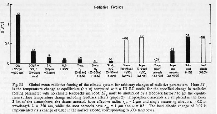
Radiative forcing of the climate system can be specified by the global surface air temperature change ΔT0 that would be required to maintain energy balance with space if no climate feedbacks occurred (paper 2). Radiative forcings for a variety of changes of climate boundary conditions are compared in Figure B1, based on calculations with a one-dimensional radiative-convective model (Lacis et al, 1981). The following formulas approximate the ΔT0 from the 1D RC model within about 1% for the indicated range of composition. The absolute accuracy of these forcings is of the order of 10% because of uncertainties in the absorption coefficients and approximations in the 1D calculations:
CO2:
where x_0=315 ppmv; X<1000 ppmv.


Their Figure B1 shows a ΔT of 1.2 K for a doubling of CO2 from 315 to 630 ppmv, together with corresponding amounts for other trace gases as shown below:
In any event, there’s nothing here which amounts to an engineerinq-quality statement. Hansen’s log formula takes us back to Lacis et al 1981, which I’ll try to locate, and the feedback discussions to Cess et al 1989. Again, I’m not saying that anything here is wrong; only that it’s quite a paper chase to try to find firm footings for the actual derivation of the formulae – something that would not occur in a proper presentation.
References:
Cess, R.D., G.L. Potter, J.P. Blanchet, G.J. Boer, A.D. Del Genio, M. Deque, V. Dymnikov, V. Galin, W.L. Gates, S.J. Ghan, J.T. Kiehl, A.A. Lacis, H. Le Treut, Z.-X. Li, X.-Z. Liang, B.J. McAvaney, V.P. Meleshko, J.F.B. Mitchell, J.-J. Morcrette, D.A. Randall, L. Rikus, E. Roeckner, J.F. Royer, U. Schlese, D.A. Sheinin, A. Slingo, A.P. Sokolov, K.E. Taylor, W.M. Washington, R.T. Wetherald, I. Yagai, and M.-H. Zhang, 1990: Intercomparison and interpretation of climate feedback processes in 19 atmospheric general circulation models. J. Geophys. Res., 95, 16601-16615, doi:10.1029/90JD01219. [I presume that this is Cess et al 1989 – check] Abstract
Hansen, J., D. Johnson, A. Lacis, S. Lebedeff, P. Lee, D. Rind, and G. Russell, 1981: Climate impact of increasing atmospheric carbon dioxide. Science, 213, 957-966, doi:10.1126/science.213.4511.957. url
Hansen, J., I. Fung, A. Lacis, D. Rind, S. Lebedeff, R. Ruedy, G. Russell, and P. Stone, 1988: Global climate changes as forecast by Goddard Institute for Space Studies 3-dimensional model. J. Geophys. Res., 93, 9341-9364. url
Lacis, A., J. Hansen, P. Lee, T. Mitchell and S. Lebedeff, 1981. Geophys. Res. Lett. 8, 1035-1038. Greenhouse effect of trace gases, 1970-80. Abstract
Luther and Y. Fouquart 1984. The intercomparison of radiation codes in climate models. World Climate Program Rep WCP-93. 37 pp
Ramanathan, V., L. Callis, R. Cess, J. Hansen, I. Isaksen, W. Kuhn, A. Lacis, F. Luther, J. Mahlman, R. Reck and M. Schlesinger, 1987: Climate-Chemical Interactions and Effects of Changing Atmospheric Trace Gases. Rev. of Geophy., 25: 1441-1482. Abstract [check ref]
Ramanathan, V., 1987: The Role of Earth Radiation Budget Studies in Climate and General Circulation Research. J. Geophys. Res. Atmospheres, 92:4075-4095. url
Wigley, T.M.L., 1987, Relative Contributions of Different Trace Gases to the Greenhouse Effect. Climate Monitor 16 14-29.


252 Comments
Once again a CS of 1.odd C and a bunch of hand waving.
It would appear that the 3C number comes from running the models against the paleoclimate reconstructions and is validated by the (odd man out) surface temps produced by Hansen. This is what the whole MWP, LIA, HO, yada yada yada fight is about. Protecting the catastrophich projections that come from the CS of 3C. Can you imagine the climbdown to a CS of 1C? No wonder nobody who has staked their messiah-hood on it can look rationally at the evidence.
Dear Steve, I would disagree with your statement that the logarithmic relationship is not a law of physics. I am convinced that it is an emergent law valid at high concentrations and it was derived back in 1896 or so by Svante Arrhenius, see e.g.
http://en.wikipedia.org/wiki/Svante_Arrhenius#Greenhouse_effect_as_cause_for_ice_ages
who also tried to use the greenhouse effect as an explanation of ice ages – which was incorrect.
I don’t think it is fair to demand all these things to be explained in a self-contained engineering way because the climate is somewhat more complicated than a wheel where an engineer only needs to know the value of pi, if I simplify a bit. 😉
The logarithmic dependence is essentially the inverse relationship of well-known laws of thermodynamics. If you have
Extra_energy = alpha ln(C/C0),
then you can also write it as
Extra_Energy/alpha = ln(C/C0)
exp(Extra_Energy/alpha) = C/C0
which is pretty much the Maxwell distribution. This “derivation” was a bit heuristic and anyway, Arrhenius’ original calculation using also Stefan’s law was flawed but I believe that the relationship is correct at high concentrations. For very low concentrations, the effect is linear (the logarithm would go to minus infinity, too bad) as can be seen by solid arguments. The square root for intermediate concentrations is just a phenomenological trick to interpolate the linear and logarithmic functions. There are other curve-fit functions being used.
The logarithmic profile is important because the greenhouse effects slows down as the concentration increases – tenth painting of your room doesn’t have much effect. See
http://motls.blogspot.com/2006/05/climate-sensitivity-and-editorial.html
We have already made about 1/2-3/4 of the temperature increase from the doubling even though we have only made 1/3 of the doubling of CO2 from 280 to 560 ppm.
By the way, I would still be interested in your comments about the vast differences between rankings of the warm years and trends according to different teams etc.
http://motls.blogspot.com/2008/01/2007-warmest-year-on-record-coldest-in.html
Ive become skeptical of the logarithmic relationship. Qualitatively it seems okay but It does not seem fundamental to me once I think about it further. As a side note, I dont like thinking about global warming as related to the net downward vs upward radiation because there are only two parameters that matter. How much power reaches earth, and how quickly that power is dissipated. For some reason it makes more scene to me to think in terms of resistances.
A resister amplifies a current to produce a voltage. It is a passive device and all it does is slow the flow of energy. Similarly the atmosphere impedes the radiative energy flow which results in a greater thermal potential difference between the earths surface and space. The gain with respect to solar forcing is proportional to the outward energy flux resistance and inversely proportional to the inward energy flux resistance.
Near the bottom of the atmosphere most energy is transferred though conduction and convection while near the top of the atmosphere most energy is transferred though radiation. These are almost parallel paths for energy flow. Resistances in parallel add as follows:
1/Req=1/R1+1/R2
For a moment lets only consider the radiative energy flow. The resitance is the inverse of the transmittance. The transmittens at a given frequency is given by:
Transmittence (lambda(f))=I/Io=1-exp(-lambda*x)
Where
x is the amount of gas the light travels thorough.
Lambda is the decay factor
I is the intensity after the light went though a quantity x of gas
Io is the intial intensity
Now if we want to consider how much light is absorbed over a single band we simply multiply by a distribution function and integrate from negative infinity to positive infinity.
For simplicity mathematical simplicity we can use a Gaussian distribution for lambda. Then the total tranmittence takes the form.
Transmittence=
Integral_{-00,00}(k(1-exp(-lambda*X))*exp(-(lambda-lambda_o)/sigma))d_lambda
If you combine the exponential terms then complete the square, you get a Gaussian distribution. The integral of a Gaussian distribution is known thus we can solve the above expression. Ill do it as an exercise later.
As a side not to be more precise we could also include the Stephan Boltzman distribution in the integral but if the band is narrow it will be roughly constant over the band.
It seems Nature is prepared to consider one other possibility..
http://www.nature.com/nature/journal/v451/n7174/full/nature06502.html
Lubo, the fact that the “law” doesn’t apply to ozone means that it isn’t a “law” as it stands. It also depends on the armospheric profile – I’ll tie this in to Houghton’s “the higher the colder” argument at some point.
I’ll take a look at your post tomorrow.
One more comment, about the feedbacks. The corrected version of Arrhenius’ calculation can be done properly today and if you neglect the effect of H2O in all forms on the atmosphere, the temperature increase from CO2 doubling is gonna be around 1 °C. Note that Arrhenius’ result was about 5-6 °C, about twice the IPCC value. 😉 But his numbers were completely wrong.
The increase from 1 °C to 3 °C or so as proposed by the IPCC is due to feedbacks and the primary positive feedback is water vapor as a greenhouse gas. With higher temperatures, you get more water vapor in the air, which also acts as greenhouse gas and causes extra warming. There are other feedbacks related to clouds and some of them are likely to be negative, version of the infrared iris effect. No one has a satisfactory calculation that would count all these possibly relevant feedbacks and got a convincing factor with a reasonably small error margin.
Moreover, there is one extra negative contribution. CO2 and H2O fight for the same spectral lines, so their mixture induces a smaller greenhouse effect than the sum of the two greenhouse effects that they would cause separately.
Roy Spencer et al., in his and their recent papers, argues that certain cloud-related feedbacks assumed to be positive are actually negative and the error was caused by an erroneous interchange of cause and effect in some observations of pairs of quantities.
At any rate, everything I’ve seen about arguments for a 3 °C sensitivity seems consistent with my statement that they first decide what the result should be and then they adjust all other arguments and ideas about what is known and what is unknown about various effects. That’s why some extreme people promote the 5 °C sensitivity even today – it’s about choosing unrealistic priors that cannot be removed by an inaccurate calculation. A realistic value is those 1.1 plus minus 0.5 °C, as calculated by Schwartz, and there are more solid ways to see it.
One of them is as observational as you can get. If you believe me for a while that I can justify those logarithms, then we have already made – since 1800 – around 1/2 of the warming expected from the CO2 doubling (and probably more once the precise function beyond the logarithm is considered and overlaps taken into account). By thermometers, it has led to 0.6 °C of warming, so the full effect of the doubling is simply around 1.2 °C. This is the most solid engineering calculation I can give you now. We will get an extra 0.6 °C from the CO2 greenhouse effect before we reach 560 ppm, probably around 2090.
We can’t know the sign of cloud feedback a priori, but don’t construe that to mean that it is possible the sign is negative.
Okay.
It seems to me that the above exposition leaves out the effect of thunderstorms/hurricanes/updrafts/typhoons in convecting heat directly into the upper atmosphere (30000 ft plus) which over-rides any effect of CO2 in keeping the heat in. Second, the behavior of clouds is so vaguely modeled that they really can’t discount Lindzen’s infrared iris theory (or Spencer’s recent result).
#7. Lubo, the fight for spectral lines is an issue that I’ve wondered about. It’s the type of thing that you’d see in an engineering study. The best article that I’ve seen on this is Clough JGR 1995, which was never cited by IPCC though Clough is not a fringe guy. I’d be interested in your thoughts on Clough online here (85 MB zipped) http://www.driveway.com/kjiye62695
Dear John and Steve,
I think no one says that the Arrhenius’ law is “fundamental” in the profound sense. The only fundamental laws are those of string theory – John A will surely forgive me 😉 – and even the Standard Model and Einstein’s equations of General Relativity are already derived and approximate! But climate science (and even other disciplines) is about a certain legitimate approximation that one can make.
It is not clear to me why the argument about ozone makes the law a non-law. If it’s valid at all, it’s valid under some simplified assumptions that are pretty well satisfied for CO2 in the atmosphere but not O3 in the atmosphere. The ozone is non-uniform, has properties that depend on the precise position in the thin ozone layer, and moreover its concentration is simply too small so that we’re not yet in the relevant logarithmic regime. O3 is very strong but there’s just a small amount of it.
But if you take e.g. the law pV=nRT for ideal gases, would you also argue it is not a law because it doesn’t hold for liquids? It is not supposed to hold for liquids. It is a law for ideal gases. The Arrhenius law is a law for gases that can be treated as uniform and that have a high concentration. It is a nice idealized law that is valid in nice idealized situations, much like all laws that physicists study. If a situation is not idealized like that, it is often an extra work for a physicist, not always a problem of a law.
Let me give you a better derivation of the logarithmic relationship, supporting why I think it is fundamental, in the next comment.
Best, Lubos
Re #7 (Motl):
You are assuming the warming can be 100% allocated to CO2 change, with no negative forcings (aerosols) included. You are also assuming the response to the CO2 increase is instantaneous, when we know that is wrong simply due to ocean heat capacity and numerous other slow responses that show Earth hasn’t yet adjusted to the change. Those issues make the increase so far consistent with a 2.5 to 3 K or more sensitivity to CO2 doubling. As is clear from reading IPCC AR4 – their numbers are at least self-consistent on this basic sort of issue.
6, Steve, in science and engineering, there are lots of “laws” that have limited scope. Ohm’s law, for example, doesn’t apply to transistors. But we still call them laws. Arrhenius’ law is every bit as general and rigorous as Ohm’s law, or Henry’s law, or 100 other “laws”.
they dont meet the standards that I expect in an engineering report … theres nothing here which amounts to an engineerinq-quality statement – it strikes me as very weird to demand an ‘engineering’ report in a field which is not engineering. Why is engineering your gold standard and how can this undefined standard be applied to other fields? Why not demand an ‘astrophysics-quality statement’ or the standards you expect in a ‘chemistry report’? Or, better – why not specify exactly what you are looking for, instead of the meaningless ‘engineering quality’?
Arthur Smith says:
That is what the GCMs say – take away CO2 and the temperature is flat. Are you arguing that the GCMs are wrong?
Why is the response to volcanic aerosols fast but the response to CO2 slow? I would expect them to be the same order of magnitude.
How did GCMs measure the effect of aerosols that they included? My understanding is they did not because there is no data available. They simply added enough aerosol forcing to make the numbers work out based on the assumption of a 3 degC sensitivity.
Lubo Motl wrote:
If a fraction of this 0.6°C warming was due to other factors, then the full effect of doubling will be less than 1.2°C. But now we’re getting near the curve fitting exercises that Hansen et al is doing.
Re Cess et al, 1989
Interpretation of Cloud-Climate Feedback as Produced by 14 Atmospheric General Circulation Models
R. D. CESS & 21 coauthors, Science 4 August 1989:
Vol. 245. no. 4917, pp. 513 – 516
DOI: 10.1126/science.245.4917.513
http://www.sciencemag.org/cgi/content/abstract/245/4917/513
I can’t find a free copy of this online. Could someone post the link, or email me a copy?
Thanx, PT pdtillmanATgmailDOTcom
Dear Steve, the overlap of the spectrum is surely an interesting aspect but still, the logarithmic relationship is kind of more fundamental. Here’s an explanation of it that should also make it obvious what one needs to assume for the law to be right.
Take Earth with CO2 only. The density of CO2 decreases exponentially with the height, being proportional to the Maxwell-Boltzmann factor exp(-height/height0) where height0 is something over 5 kilometers, I don’t know exactly, for CO2. The precise number doesn’t matter for the qualitative result.
This exponential decrease is standard result of college thermodynamics, coming from the maximization of entropy of a gas given a conserved energy. I can remind you about the derivation if you needed it. 😉
Now, if you increase the total concentration of CO2 e-times, the level where the concentration is equal to a reference value, say C0, increases exactly by height0 (up). I conveniently choose C0 to be a representative for the concentration above which the whole atmosphere may be considered transparent for the infrared radiation we consider, with some accuracy. The height where this concentration is C0 may be referred to as the tropopause, the boundary between the troposphere and the stratosphere above it. It is somewhat fuzzy but I can choose a convention about the percentage how transparent it should be, and then the tropopause will be a well-defined sharp shell.
The fun is that the behavior at the tropopause is pretty much universal, regardless of its height. The other assumption I need to use is a pretty much constant lapse rate – the decrease of the temperature with height above the Earth. This is another “law” I need to assume, with all disclaimers about its inaccuracy etc. The lapse rate law holds because it is a form of the adiabatic law. See lapse rate at Wikipedia.
So if the multiplication of the total CO2 volume by “e” lifted the tropopause by height0, the temperature at the tropopause dropped additively by the lapse_rate times height0. Because the lapse rate is about -5 °C per kilometer, you will get about 25 °C decrease of the tropopause temperature from multiplying CO2 by “e”.
A linear decrease of the temperature means that the radiation that is emitted by the tropopause decreases by a linear term, too.
Now, I must impose the overall equilibrium of incoming and outgoing energy. So if the tropopause radiation dropped by a certain amount E and the incoming solar radiation is unchanged, the radiation directly from the Earth surface must increase by E to compensate the drop from the tropopause, which means that the surface temperature must increase by a linear piece.
So if you combine all these things, you see that a geometric increase of the total CO2 volume – and I could have divided the “e” times increase to several smaller fixed percentage increases – means a linear increase of the surface temperature. This conclusion is valid assuming that various linear relationships mentioned above hold. So the lapse rate should be pretty well-defined i.e. constant between the old and new tropopause; the change of the percentage of energy emitted by the surface vs tropopause should be much smaller than 100%; the predicted change of the temperature should be much smaller than the absolute temperature of the surface, and that may be it. Then the linearizations mentioned above are legitimate.
With these assumptions, and they are pretty well satisfied for the doubling from 280 to 560 ppm of CO2, just check it (the temperature change about 3K is much smaller than the 300K absolute temperature, the percentages change from 90:10 to 91:9 or something like that), the Arrhenius’ law is a law. It is all about the Maxwell-Boltzmann distribution. A geometric/exponential increase of the concentration moves the physical phenomena linearly in altitude and makes standardized linear contributions to various terms.
Best wishes
Lubos
Re Lubos 3, 7, etc
Over at http://www.climateaudit.org/?p=2086 I asked
More and more, I think so. Be nice to know, eh?
Lubos, thanks for these thought-provoking posts.
Cheers — Pete
Raven, you are a good poster but I’m afraid that the statement that, when CO2 is taken away, temps are flat. If you subtract CO2 with a sensitivity of 3, you get cooling. This means that you haven’t removed the other anthropogenic effect: aerosols (some of them) and once that is removed, if it still trends down, you’ve done something wrong becuase the sign of the solar effect is positive. In fact, if it’s flat, it’s also wrong for that reason.
Oops, that should be, “temps are flat, is wrong“
Re: more homework
The WGNE Workshop on Systematic Errors in Climate and NWP Models (San Francisco, February, 2007) has a number of pertinent papers & prsentations that I don’t recall seeing discussed here:
http://www-pcmdi.llnl.gov/wgne2007/presentations/
The one I’m studying right now is right on-topic for here:
Bill Collins, Radiation errors in climate models
Click to access wgne_Collins_021207.pdf
–lotsa slik graphics, aimed at my level (ie low).
Enjoy! PT
Re: WGNE
Gotta love a group that doesn’t take itself too seriously:
Click to access mm_acronyms.pdf
PCMDI: Principal Cause of Modeler Diatribes and Incentives
PCMDI: Persons Culpable for Most Data Indigestion
PCMDI: Pretty Clever Methods for Dodgy Information
NCEP: National Center for ECMWF Predictions
ECMWF: Every Climate Model is Woefully Faulty
WGNE: Whats Good is Never Easy
WGNE: Weve Got Never-ending Enthusiasm
Thanks, Pete! I forgot to complete the calculation so that it has all the numbers and one actually ends up with the 1 °C sensitivity. 😉 First of all, fundamental physicists respect “e” and not “2” as the right base of exponentials 🙂 so the goal will be to show that multiplying CO2 volume by “e” will warm up Earth by a certain amount comparable to 1 °C / ln(2) = 1.44 °C. 😉 Let’s see how close to 1.44 °C for this e-normalized climate sensitivity we can get.
With the e-multiplication of CO2, the tropopause shifts by height0 = 5 km, the temperature at the tropopause drops by 25 °C. If the tropopause and the surface were emitting 50% of the radiation each, then the surface would have to warm up by 25 °C. That would be a pretty high e-sensitivity. 😉 Fortunately, the surface emits a vast majority of the radiation, so a small increase of the surface temperature is enough to compensate the small cooling at the tropopause.
Assuming the average percentage composition of the radiation from surface vs tropopause to be 94:6, you see that the Earth is 17 times more important than the tropopause for the energy budget. So you need to change the Earth surface temperature by 25 °C / 17 in the opposite direction to compensate them which is 1.47 °C. A pretty good agreement. OK, I cheated a bit but what is important is the framework of the calculation. You may try to put better numbers into it if you want to improve it. 😉
Re: 22, Bill Collins, Radiation errors in climate models
Click to access wgne_Collins_021207.pdf
THE slide for here is his #15, comparison of 12 current GCM’s CO2 forcing results. 3.67W/m2 ± 0.28, 5 to 95% CI is 3.2 -> 4.1. Source: IPCC AR4
Nice slides, Bill!
Cheers — PT
Arthur #12:
You are assuming that the lag due to oceans and such is more than a a couple of years.
You are also assuming that the value of 0.6C is not contaminated by UHI and microsite issues.
Ah, the usual matter of scattering all the information all over the various AR chapters and multiple literature sources.
How exactly does CO2 instantaneously double, consistitute the radiative heating, provide 4 Wm-2 (???) up and down, and exist with fixed surface-troposphere climate parameters? And what about all of these other factors?
What bearing upon reality could a forumula derived from such a bizare unnatural climate scenario have, even forgetting about clouds and water vapor and wind and lapse rates and….
You are also assuming that whatever the amount of warming, it is 100% due to CO2 and it’s direct feedbacks. Even the IPCC has admitted that up to 1/4th of that warming is due to the sun. (I personally believe the value is closer to twice that amount.)
I think the point is that the climate modellers (Hansen and Wigley) employ mostly linear mathematics without any reference to fundamental physics of the behaviour of gases (ie quantum theory). In this particular case, they both refer to their own previous guesses as justification for their assumptions.
Thus the explanations in AR1 are circular and not at all insightful.
Dear Arthur #12,
your concerns (and objections against my simple calculation of the sensitivity based on observed temperature increases) are easily seen to be irrelevant. First, aerosols have nothing whatsoever to do with the calculation of the CO2 sensitivity. CO2 sensitivity is about the contribution of CO2 changes to the energy budget and to the temperature while aerosols are a different, largely independent contribution to these quantities. So it is not clear why you mix them up.
Second, the effective time constant associated with upper oceans’ heat capacity is about 5 years. It means that the oceans can store most of the heat “in the pipeline” for 5 years or so, see e.g. Stephen Schwartz’s paper and its references and followups. According to others, it may be 10 years, but you simply won’t delay warming effects by 50 or 100 years. If there were 1 °C of warming “waiting in the pipeline” at least since 1998, I assure you that most of it, (1-exp(-2)) times the full amount, would have already occurred between 1998 and 2008. Because we didn’t see warming by 1 °C in the last ten years – in fact, 2008 was 0.41 °C cooler than 1998 according to RSS MSU (but the overall trend is about zero), your conjectured huge temperature increase waiting in the pipeline is in a very bad shape and I would say it is falsified.
Deeper oceans may cause longer delays but the heat exchange with deep ocean is so slow that it is negligible.
Deep ocean circulation takes 2000 years but after a few centuries, oceans are also able to absorb the extra CO2 and undo our addition of CO2 into the atmosphere which is why it makes no sense to think about heat storage of deeper layers of the ocean. You can’t kill my arguments in these very naive ways because the argument is very robust. Also, let me say in advance that it doesn’t matter whether we consider the bare sensitivity or the sensitivity including feedbacks. The logarithmic relationship applies in both situations as long as the feedbacks are proportional to the bare warming caused by CO2 which is a good approximation for water vapor and similar feedbacks.
Best
Lubos
Hello all – this has been a fun read the last few days. Quick question that I haven’t seen addressed elsewhere (if it is, please please send me a link so I can read and not disrupt this conversation by sidetracking it).
GCM’s predict X amount of warming given Y amount of CO2 concentrations. Since 2000 it seems the temperature anomalies have remained static regardless of what method the data was accumilated eg satellite or ground temps. (some are giving that static temperature as higher than others, but as a whole, all seem to be static). How long will the temperature anomalies have to remain static before AGW is seriously rethought? Or, will AGW activists simply state that a delay is to be expected? If so, what length of delay would “prove” the GCM’s incorrect? What would a noticeable sustained drop in temperature anomalies – say back to 1990-1997 levels – do?
An audit site seemed the only place to ask this.
AJ
I forgot to say. If you, Arthur #12, meant that the actual CO2 warming since the beginning of industrial revolution should have been more than 0.6 °C because the aerosols added cooling, then you are counting something that you shouldn’t be counting. Unlike CO2, man-made aerosols don’t survive in the atmosphere for decades or centuries. If the 1945-1979 warming is explained by aerosols, it’s OK but the aerosols from that time are already gone and their cooling has been undone.
We produced much smaller ratio aerosols/CO2 in the last 10 years than in the 1960s because the smoke is largely gone while CO2 production continues. Because we don’t produce so much aerosols, it also means that aerosols contribute much less to cooling than they did in the 1960s: they’re no longer in the air. In the 1960s, aerosols created roughly as much cooling as CO2 did warming, by assumption, and today it is much less – because our chimneys are cleaner – which justifies me to neglect the aerosol contribution between 1800 and 2007: their cooling has been mostly undone once we heavily reduced their production.
Numerically, you could change 0.6 or 0.7 to 0.8 °C from CO2 but you won’t change it to 1.5 °C by adding an aerosol story that you would need for a 3 °C sensitivity. Incidentally, your choice of aerosols is cherry-picking. We could also argue in the opposite way, that some of the 0.6 °C was caused by natural warming effects (e.g. solar), leading to an even smaller CO2 sensitivity. What I did in the simple calculation above was based on a neutral assumption that what we see is what we get by CO2 only. Unless proven by solid arguments, any other accounting is a form of bias.
The atmospheric impact of HOH is necessarily far more complex than CO2 simply because the presence of CO2 for most of the atmosphere exists only in the gaseous phase while HOH can exist in all 3 phases…gas, liquid and solid. Loehle (post #9)I believe correctly, points out that the presence of HOH as a prime contributor to, and an exploiter of, convection is thereby a direct transporter of heat from the surface to the tropopause. This is accomplished through the acquisition of latent heat through surface evaporation and the return of latent heat through condensation back to liquid, or condensation plus sublimation to ice at a range of altitudes which encompass the whole troposphere. HOH is also a self contained transporter of negative temperatures from the altitude of condensation and/or the initiation of precipitation, back to the surface.
If one logically assumes that the higher the surface temperature of bodies of liquid HOH at the Earth’s surface, the greater the overall cloud-cover and redistribution of heat through the lower atmosphere, then the lack of emphasis of HOH’s contribution to GW in deference to CO2’s almost totally radiative effects, are hard to reconcile.
The reason might be that atmospheric scientists in the public arena try to stay away from those processes they really don’t understand but can nevertheless promote through simplistic bafflegab. For AGW proponents, CO2 seems to provide their low-hanging fruit.
As an OT metaphor:
Have you ever seen a recent paper on ball lightning? The only things your read if you can find them, are discussions of whether the phenomenon exists or is an illusion. As with the current status of the MWP, there are ample, highly credible observations of the kugelblitz over the past several centuries, but few scientific papers acknowledging the phenomenon. And, as in the case of AGW, there are few coherent theories to provide a definitive and unequivocal understanding of this stmospheric electricity phenomenon.
Finally, science should be involved in solving physical mysteries and should refrain from altering the past to promote political and/or social agenda.
32, except that aerosols are also spatially limited. Europe and North America are producing a lot less aerosol per kg of CO2 than in the 1960s, but it’s still pretty bad in Asia (“Asian brown cloud”). You would expect that there would be a significant contrast in mean temperature between China and the ROW if aerosols are that significant a forcing.
Larry, I think you mean that China should have a less pronounced trend, right? Does anyone have a chart of this? We will have to be careful, of course, since the quality of the data may be suspect.
I think this is one:
I notice that the the Northeast US, Europe, and southeast China show less of a trend (or even cooling) versus than the surrounding areas. What do you make of it?
18, 24 Lubos
Very neat. As a theoretical physicist myself (solid state) I can appreciate the facility with which you work the numbers and agree with most of what you say.
However, I have a couple of issues:
– You say in 18: A linear decrease of the temperature means that the radiation that is emitted by the tropopause decreases by a linear term, too.
That is only true if we are talking about a small decrease in temperature. Did you intend to put in “small”?
– This one is more important, I think. You say in 24: the surface emits a vast majority of the radiation.I’m not sure whether you are talking about radiation in general or photons which escape absorption and carry energy off to the stratosphere, and away. If it’s the former, OK. If the latter, I disagree — I would suggest that photons leaving the surface are almost all absorbed by water-vapor (thermalized and re-emitted with different wave-numbers) before reaching the tropopause.
35, for the period of 1951-1980, there would be more aerosols in North America and Europe than China. I would expect that to be reversed now. The Asian brown cloud can be seen from space:
http://en.wikipedia.org/wiki/Asian_brown_cloud
There’s nothing subtle about it.
If the oceans are absorbing CO2 … its ppm are still rising … yes/no? As for natural causes, I am waiting for an engineering-based explanation for how they work — i.e., more than simply saying “sun warmer = observed warming.” Also, what’s good for the roses in a hot house aint necessarily so good for all of life on earth.
Okay Larry, but as far as trends go, what does that mean? What is the evidence for and against any significant effect from aerosols, and what is the expected magnitude and sign? I’m not sure we actually know, given the charts I’ve seen!
39, I think the spottiness in China simply indicates that their data is sparse. I don’t know that we have good enough information to draw any conclusions.
John A says: (January 4th, 2008 at 3:12 pm ) “they both refer to their own previous guesses as justification for their assumptions”.
Ah, yes. If you carefully follow the arguments in most of these discussions, that is exactly how the authors “prove” their point. I went back and reread a couple of Ramanathan’s papers and he is oh, so expert at it. I’m still looking for a definitive quantitative assay of CFCs in the stratosphere. Ramanathan starts by saying they might be there, and then calculates to great precision what their effect would be if they were there, and ends with those as THE results, never actually giving any reference to observation of existence of the CFCs or measurement of density. Look closely at the sleight of hand, where the original “let’s start here” proposition is eventually cited as proof. AR-1 is a minor example. They get better with practice.
Thanks Andrew,
As Lubos points out those aerosols shouldn’t be an issue any longer, if they ever were.
Anyone else care to give a possible explanation for the missing contribution expected if the postulated positive feedbacks are correct?
Because of the extra warmth there are more butterflies in the air blocking tne sun!
Eric
The group asking for trillions of dollars is the one who should provide the clear exposition. Advocates of solar TSI, cosmic rays, etc, are not asking to reach into my pocket, with the exception of the CLOUD experiment.
45. 3 days of testing over 1.6% of the worlds land mass and you want to draw conclusions?
Sorry I seem to have been involved in an OT excursion.
The 4 major non-water greenhouse gas charts all have the same basic shape. Leading me to believe it’s not CO2 making the other 3 go along, but rather they follow either temperature and/or water vapor. Or something else. Don’t let 33% more CO2 over 120 years scare ya.
Be that as it may.
Almost all of the anomaly trend is since 1980ish. Except for a few lower anomaly years here and there. Since around 1995 none of the monthly figures (GHCN 1880-11/2007 + SST: 1880-11/1981 HadISST1 12/1981-11/2007 Reynolds v2) are negative or even under 10 or so.
Something’s changed.
Re: Fig. B1., the Radiative Forcings, it seems the rating of HOH at only 4% of CO2 is low, considering there is so much more HOH, and I thought HOH had a relatively high heat capacity amoung natural substances.
re 53. Actually a standard of “beyond a resonable doubt” would be a good standard for
implementing any government policy including policies on Global warming.
Would you put somebody to death based on the quality of AGW evidence?
I wil be posting chapter 13 “Thermodynamic feedbacks in the climate system” from my text “Thermodynamics of Atmospheres and Oceans” on my website, hopefully this will be up on Monday, i will post the location once it has been uploaded. This is fodder for first year graduate students, so not exactly baby food.
Re #7
In a solid engineering calculation you’d actually get the math right although you’ve improved over what you had in your blog, if you do it right you come up with an additional 0.76 so overall about 1.36
re 62. Thanks Dr. Curry.
Re 60, 63 Papertiger
Have a look at Collins slide 5 at
Click to access wgne_Collins_021207.pdf
Energy in (from sun) = Energy out (from reradiation)
Cheers — Pete Tillman
Andrew says @January 4th, 2008 at 2:39 pm
Look at http://ipcc-wg1.ucar.edu/wg1/Report/AR4WG1_Print_Ch09.pdf Figure 9.5
You will notice that there is a mysterious step change down with the Angung volcano but after that the trend is basically flat or a very slight downward trend. From this graph you can the IPCC attributes a 0.75 degC rise due to CO2 since 1960.
I find this graph interesting because it seems to imply that we would be stuck in the LIA if we had not dumped CO2 into the atmosphere.
Re #6
That’s because Motl’s concept of the cause of the log relationship is not the actual cause.
The log relationship derives from the lineshape of the spectral lines (Voigt profile) when the centre of the line is saturated and the further increase in absorption due to increase in concentration is in the wings of the lines. That’s why not all species will show such a dependence (i.e. CO2 vs O3).
To expand on my point about convection, compare the predominant weather (when there is not a front passing) in the winter in the NH. Flat low clouds, no updrafts. As it gets warmer, you get updrafts, cumulus clouds and thundershowers. In the South in the summer it was common to get a shower every day at 5pm from these clouds. Is this not a negative feedback? How effective are these convection systems at pumping heat away from the earth? I am guessing that this is much too small scale for the GCMs to include. Judith?
Thanks Raven. As you can see earlier i said:
So this is a puzzler. How did they manage to get it to do that?
Additionally, I notice that they over estimate the effect of volcanoes on the climate. I know I’m not the first one to notice it, either. Nir had something about it:
#71 Craig Loehle
This vertical convection issue (in both atmosphere and ocean) is why I don’t understand how anyone could argue for 1D EBMs. The strongest negative feedback is going to come from things only a coupled AOGCM can give you. Forget the past. The future is not linear.
I am particularly interested in learning how the GCMs cope with ocean thermohaline upwelling. Deep ocean heat brought to the surface in Hurst-like pulses, and the effect this might have on ocean clouds. With an engineering-quality document I could turn to chapter X, page Y, Figure Z, Equation 1.4.2.2 and see for myself exactly how this issue is treated/ignored. It would make audit SO much easier.
Andrew,
From the IPCC report I linked to:
That seems to indicate that they choose only the simulation outputs that gave them the results they wanted to see given their assumption that CO2 is the major driver.
#66 Raven. This comes back, I believe, to Browning & Vonk, on convergence. There is no convergence in these models, so they choose sub-ensembles that make it appear as though there is convergence. Ultimately, I defer to an expert. My only reason for chiming in is to get this observation linked to “exponential growth in physical systems”.
There are algorithms based on observation-experimentation that are liable to know the real delta F, the real absorptivity, emissivity, total emittancy, etc. of carbon dioxide. I’ve applied many of them and found the radiative forcing proposed by the IPCC team is not real.
While I’m afraid I didn’t understand that, your assessment seems correct to me, Raven. Either way it’s obvious that there models of “natural” forcings only are either flawed, or include something I’m not aware of. I bank on the former.
Raven said:
1. If a model’s simulation was thrown out for having MORE than 0.2°C per century, were any thrown out because of a MIN (and what was the min?)
2. There were only 19 simulations chosen from the five models run. Before the purge, how many simulations were run (total). I guess what I’m asking, were more sim results over 0.2°C/century, or under?
3. Did they say what the “natural forcings” were? Their line has been the increase in CO2 is not “natural”, but man-caused.
Well, henry, I know they have an attribution to solar, and from what I can tell, they do include volcanoes (but over do it, see above)
I think I get it now Raven, they eliminated any models with a big variation. They hand picked a bad fit.
I think you do want to be a little careful possibly overinterpreting that ambiguous wording. When they say they censor the “control simulations” that show “excessive drift”, I think by “control” they mean the simulations that have CO2 absent. As in treatment vs. control. This is only a guess. But the logic would be that if the control runs drift, then the treatment runs would drift too, therefore eliminate them both. I am not at all certain of this. Merely highlighting the ambiguity, some possible misunderstanding, and need for audit.
I note, first, that “drift” is what you expect to happen in a Hurst-like world. Second, maybe THIS is why Gavin Schmidt insists the internal variaiblity in climate is “low”. They’ve artificially made it low in their model sub-ensembles, and they take their models as reality. Again, mere guesses.
#70 Phil,
That’s what I thought, but then isn’t it a bit more complicated than that? The CO2 spectrum is a mess, and the lines are pressure-broadened (so they’re likely to change width with altitude), in which case they’re gaussian, but that too is an approximation in the wings, and it’s the wings that count. Then there’s overlap with water vapor. All in all, is there an easy demonstration that the log relationship still holds apart from very simple situations? (Disclosure: as a laser physicist, I know a bit about spectroscopy, and actually did a Masters on Doppler-free nonlinear spectroscopy, so you can skip the basics if you reply).
#72-73 GCM’s used to drift a lot, and they used something called “flux adjustment” to eliminate that. Apparently more recent models do not use flux adjusments. But maybe they still drift. It’s sometimes hard to tell when you read the articles. In any case, from what I’ve seen, models never show the variability that is observed in the real world. A good example is albedo. Once measurements started to come in from satellites, they showed a variability that was unseen in all models, with equivalent forcing (fluctuation in radiative budget) larger than the entire CO2 post-industrial forcing. But, hey, the data must be wrong…
It’s also useful to remember that GCM’s dont know anything, apart from what we tell them. If the modeler tells the GCM that solar forcing is small, it will end up being small. The small value of solar forcing is not a “result” from the GCM, it’s an input. The input to all GCM’s tell them that CO2 is the most important forcing, so why would it be surprising that they can’t show any warming without CO2? No magic here. But that’s also why it’s important that past variability be as small as possible.
House of cards…
P.S. my previous post was a reply to post #62. Some posts disappeared while I was writing…
I’m glad you choose the term ‘house of cards’ Francois. I used that term a month or so to describe the AGW hypothesis – knowing how much attribution hinges on the GCMs – and got raked for it. But it is apt, in the sense of a complex structure contingent on the integrity of dozens of other substructures – many of them somewhat questionable.
The following link is very relevant to this topic:
http://brneurosci.org/co2.html
Note that hyperbolic functions and negative exponentials have been proposed as alternatives to the logarithmic function.
#64
If the “net solar is .5, and net aerosols = -2C, would not the absence of aerosols mean a warming of 2.5C caused by solar?
I mean … aerosols don’t cause cooling. Aerosols cause solar radiation to be reflected back to space which results in cooling.
Lots of extra sunshine since 1990 can account for all post 1990 warming if only 50% (or less) of the aerosols are being eliminated in the NH.
http://www.sciencemag.org/cgi/content/abstract/308/5723/847
I think the debate on weather solar or radiative forcing is more significant is misleading. Greenhouse gases amply solar forcing.
I noitced that there was a spectroscopy physics on this board. I found the following interesting:
http://www.john-daly.com/artifact.htm
What I would like to know is how much does limits of sampling in spectroscopy equipment effect our knowledge about the absorption band properties of CO2?
Re #73
Not at all.
Do you know where I can get a list of the CO2 infra-red absorption bands (in instantaneous transmittance per unit length) and the spectral width of each band. I’m googling radiative transfer codes but I would like something more basic for back of the envelop calculations.
Oh, these are the websites I’m looking at:
http://www.mathworks.com/matlabcentral/fileexchange/loadFile.do?objectId=7994
http://rtweb.aer.com/lblrtm_frame.html
Here is a fun experiment with Excel
Create a random series with this formula: C1+NORMDIST(RAND()*B2-B2/2, 0, B2/2, TRUE)*B2-B2/2
Where C1 is the previous value
B2 is the amplitude of random deviation.
Plot the result over 500+ samples and look at the trends – you should find lots of 20-30 sample periods with discernable trends.
In fact, I was able to frequently produce a plot that looked like the temperature variations over the last 500 years.
This silly experiment suggests that any temperature trends observed could be a result of a purely random process and that searching for a ’cause’ (human or natural) is a waste of time.
I screwed up on the normal distribution formula – I was trying create a random variation with a guassian distribution, however, the formula I posted does not do that. A simple linear random source (C22+RAND()*B23-B23/2) produces similar results but a guassian distribution would be a better reflection of the climate system if I can figure how to get excel to give me such a distribution.
Bender (#60),
I mentioned to Pat Frank that I have been considering reviewing a recent
“peer reviewed” manuscript by Williamson et al. on numerical convergence tests of various atmospheric model dynamical cores (i.e. no physics so closer to the runs I made on the exponential growth thread) for some “benchmark” cases. I would provide a review with pointed questions and remarks as seen by an applied mathematician and numerical analyst so that all of the flaws in the manuscript can be seen. If Steve M. would like to post the review on his blog so readers can see just how many manuscripts
get thru the peer review system without the essential scientific points being addressed (either intentionally or inadvertently),
you can ask him to make a copy of the manuscript available on his website
so that I can point to the problems line by line. I will include references
as I go to back up my comments and for further reading for those interested. If either of the coauthors want to respond to my review, I would be happy to engage them in further discussion if they answer the issues I raise by making some trivial additional runs.
Jerry
Dear Pat #36,
thanks for your insightful comment.
1) Absolutely, it was assumed that the change of the temperature is small compared to the absolute temperature so that one can linearize the problem. I think I wrote it but frankly, the log shape could be unaffected. For example, the log of a power of “x” is still a multiple of a log, after all.
2) I agree that when water is included, which I explicitly avoided, a part of the radiation from the surface is absorbed and reemitted. To be honest, I didn’t do the calculation with this effect of water re-emission included but my guess is that it won’t matter for the log shape. It may matter for some detailed numbers, but assuming a universal concentration of water, I believe that even with this effect included, the sensitivity will be around 1 degree C. Only when one adds the increased concentration of water vapor, it becomes those 2-4 degrees. Cirrus clouds etc. probably bring it back to 1 degree or less.
Dear Phil #55,
I agree that the broadening of the spectral lines also matters for discrete spectrum and probably leads to a log but have you actually evaluated how much it gives? It is pretty normal to obtain logs in something that is slowing down almost to zero but not quite. But it doesn’t mean that every effect that does so is important relatively to others.
Let me sketch why the broadening would contribute.
Spectral lines don’t have quite sharp frequencies when other effects are taken into account. The molecules of CO2 move, and by Doppler effect, the characteristic frequency they emit changes with velocity. Because the velocities of the molecules have the Maxwell-Boltzmann distribution (again) which is Gaussian (exp(-v^2)) in velocities, the Doppler broadening will have a Gaussian shape, too. It decreases very quickly as you go from the center.
Other effects create a different shape. For example, the spectral lines are emissions from metastable sources and they have a width. It leads to a Lorentzian shape, 1/(1+x^2), that decreases much slower for larger x. The Voigt profile you mentioned is the convolution of the Gaussian and Lorentzian shapes, a rather convoluted function. For large enough “x”, it is the Lorentzian feature that survives and dominates.
The middle of a line is saturated – CO2 absorbs nearly everything – while the “wings” are slowly saturated.
But the Voigt profile is an irrelevant concept in this case of the greenhouse effect because CO2 absorbs in whole bands, having many lines there.
The shape of the bands would be more relevant, and certain transitions have very small cross sections or decay rates.
I think that in order to disprove “my” effect, you would have to find an error in it, rather than just to say that it is “not the explanation”. Even if one is very rough, I think it has been demonstrated above that it leads to sensitivity that is comparable to a degree. You would have to show that “wings” can do it, too. Please, try to be more specific. But even if you explain your effect somewhat more quantitatively, it won’t remove mine.
Incidentally, for Steve, this 2007 paper argues that the effect of the overlap of the spectral lines is insignificant in the middle-lower troposphere.
http://www.springerlink.com/content/n876kv52n00jh542/
Best wishes
Lubos
Re: 13
A bit off topic.. but this statement seems incorrect to me.
“Ohms law, for example, doesnt apply to transistors.”
Are you sure about that? I=V/R. The change in a transistor’s current flow, as controlled by the base current flow, can be thought of as a change in resistance of the transistor, can it not?
Sorry, now back to our regularly scheduled program…
You know, I am somewhat skeptical of the above statement. I take measurements using wideband solar irradiance monitors for solar power systems. There is a website at the University of Nevada Las Vegas that has a lot of this data online. There is as much as a 100 watt per meter squared lowering of the received radiation at ground level on humid and or pollution laden days. This decrease below the nominal 1000 watts/m2 has a noticeable effect on the output of solar panels (10%) so this cannot be an instrumental error. I live here in the south where water vapor is quite prevalent in the air during the day and the same thing happens here.
I think that there are a lot of assumptions made about what water vapor does and does not do, without very much experimental evidence of what actually happens. Las Vegas is a great test case as the humidity is normally low and when there are increases in humidity or pollution you can peruse the data on a day by day basis and notice wide swings in the actual amount of wideband sunlight reaching the ground.
Data rules.
#81, I think the I-R profile of a transistor is like a diode in series with a resister. I diode behaves roughly like a voltage bias well a resister is like the derivative a the voltage with respect to current. Anyway, so in in conclusion I think V=IR applies for transistor but V is the voltage across the transistor minus the reverse voltage bias while R is the derivative of the voltage with respect to current.
Re #80
I’m afraid not, you’re relying on a cartoon version of the spectra, try looking here: http://www.agu.org/pubs/crossref/1997/97JD00405.shtml
Also CO2 has much of its effect in the upper troposphere and lower stratosphere where lines are narrower and the Lorentzian is likely to dominate.
I was looking though some of the LBLRTM files and I found this interesting:
http://ftp.aer.com/pub/anon_downloads/aer_lblrtm/
**** molec = 2 CO2
Summary for the molecule:
# lines min freq max freq min intensity max intensity
60805 442.00554 9648.00708 1.06000D-28 3.52500D-18
****** molec = 2 CO2
Summary for the molecule:
# lines min freq max freq min intensity max intensity
60805 442.00554 9648.00708 1.06000D-28 3.52500D-18
iso isotope # lines sum intensity f_wdth s_wdth #s_wdth abs_shft #shft #neg_epp # cpl
1 626 27124 1.10932D-16 0.0710 0.0898 27124 0.00284 34 0 25792
2 636 8838 1.13518D-18 0.0715 0.0912 8838 0.00284 34 0 8322
3 628 13313 4.46909D-19 0.0717 0.0916 13313 0.00284 68 0 0
4 627 6625 8.19650D-20 0.0717 0.0917 6625 0.00284 68 0 0
5 638 2312 4.71548D-21 0.0717 0.0912 2312 0.00284 68 0 0
6 637 1584 8.69966D-22 0.0724 0.0934 1584 0.00284 68 0 0
7 828 721 4.38235D-22 0.0718 0.0917 721 0.00284 34 0 0
8 728 288 1.41049D-22 0.0714 0.0902 288 0.00284 68 0 0
Total: 60805 1.12602D-16 0.0714 0.0908 60805 442 0 34114
Is the CO2 spectrum ever complex, 8 isotopes and 60805 spectral lines! Wow!
This NASA press release doesn’t seem to have reached the mainstream news yet,
–“there are substantial changes occurring in the sun’s surface and has concluded they will bring about the next climate change to one of a long lasting cold era” — “verified the accuracy of these cycles’ behaviour over the last 1,100 years to temperatures on Earth, to well over 90%” — “the general opinion of the SSRC’s scientists is that it could begin even sooner within three years with the next solar cycle 24” Which incidentally, appears to have started with a reversed polarity sunspot on the high latitude northern limb.
So they may have solved where the main heating came from, and we may soon be grateful for the CO2
OK http://.spaceandscience.net/id16.html
Dear Phil #84, the paper you linked to confirms what I wrote, namely that you can’t describe the spectrum as separate Voigt profiles. They assume that the discrete lines have Voigt profiles but study how important the line mixing is. Their result is that the line mixing is essential which means that one should better describe the spectrum in terms of bands and the Voigt shape doesn’t help at all to analyze the full absorption because it is only relevant for individual line not interacting with others too much.
It is true that with the assumption of the isolated lines, the Lorentz portion dominates for the questions of saturation but it is not your contribution to the discussion: I wrote it in comment #80.
Whether CO2 has most of its effect near the surface or the upper troposphere and stratosphere depends on whether you look at greenhouse models or reality. The warming observed in the real world that is hypothetically caused by CO2 occurs mostly near the surface. It may be a good idea to be more accurate when talking about these things – models and reality give contradictory answers about this issue.
Indeed, theoretically, the critical altitude for CO2 greenhouse effect is near the tropopause, see my comment #18.
Use of the term “positive feedback” kinda winds me up. Positive feedback is hopelessly unstable and rather boring in physical systems.
Take water vapour as an example. I could go along with the notion that atmospheric water vapour (“V”) is part of a genuine positive feedback process atmospheric temperature (“T”). But to leave it at that seems rather unphysical. This proposition suggests T and V will spiral upwards until something saturates.
At saturation, something else (call it “X”) comes into play and dominates physcal behaviour. The system will tend to resist change from the saturation point and you then have a negative feedback system where T and V are a function of X. T and V will only then act as a positive feedback response to changes in X. In physical systems, you then need to loof for things which alter the physical property X.
That does not to stop other factors from causing changes to T or V. An increase in T can result in an increase in V (to maintain the saturation). But it means the (claimed) positive feedback loop is no longer in play.
So let’s say a change in CO2 drives up T. And (for argument’s sake) the factor X is closure of the LW bands. Because T increases, V will respond to maintain the saturation. But there is no physical basis to argue that the change of V will amplify the change of T – you need a change of X for that (i.e. something which opens the closed bands).
That’s one reason why I feel skeptical about the claimed “stable positive feedback loop” which is used to effectively double the response of T to CO2.
re. 82 83 Julian Braggins.
It is NOT a NASA release. Please read Leif Svalgaards comment
in Svalgaard #2
Re # 90 Jordan
Well said.
There have been speculations as to whether certain responses are linear, logarithmic, exponential, hyperbolic or whatever seems fashionable. Sometimes it is postulated that a resonse can change from one category to another. Well, it can. Examples are the physics of ice/water/steam or the transition from laminar to turbulent flow. However, in the real world, such response shape changes are usually associated with an identifiable event such as a change of phase.
Can onyone provide an example from nature where a response curve changes gradually from one type of math to another? For example, do we have mercury thermometers with linear calibration at room temperature and exponential calibration near boiling point? I think not.
Such change of phase or similar has its own implications as you note, Jordan, regarding feedback.
In a column of atmosphere, it is hard to see the spectral absorption properties of a gas like CO2 undergoing a change of maths as above. Sure, a gas might freeze as it gets colder, but the model should note that. The shape of the response curve must have a basis in physics. A basis in measurement is insufficient. When one is dealing in high powers like T^4, tiny differences can become important. But all this is of little realism when albedo of earth is taken at 0.3, yet derivations from it use 3 significant figures. Mathemeticians, please intervene!
Absent sudden phase-like changes, we address questions like “why does ozone absortion differ from CO2 abdorption?” The answer is easy. CO2 stays as a relatively stable molecule, while ozone is highly reactive and reactions are commonly exothermic or endothermic.
Ozone is interesting, because it is mainly implicated in the question of why there is a cold region (tropopause) when heat radiating from the sun meets heat coming the other way from earth radiation. Heat + heat = cold? There is so little ozone that the reduction in temp, to something like minus 80 deg C, cannot be caused by ozone absorption. If ozone is implicated, it has to be by reactions that change it to another molecule. Where is the physical evidence (as opposed to whiteboard equations) of such reactions? How good have original ozone layer models and CFCs proven to be in the last 30 years?
As one goes higher above the tropopause, it warms up again. There are many model calculations of heat emission and absorption made in the vicinity of the tropoause, but why is the atmosphere above it neglected? It might be of low density, but it still has enough molecules to record a temperature and this temperature can be changed. I have not seen it mentioned in any models, but I have not studied all the models. It is important in polar regions if sunlight heats it, because calculations I have seen of solar irradiance take the radius of solid earth an an interceptor and neglect the gaseous layer around it.
I have yet to discover if models allow for radiation to occur on the night side of earth. If they do, it it treated as a disc or a hemisphere?
In similar vein, is irradiance from the sun from the disc alone, or from the corona as well?
One could go on and on.
First get the postulated theory tight, then confirm or deny by measurement, then draw deductions and consequences. That is the right order for science. It is not being used when the IPCC prints FAQs then Orders for Policy Makers before presenting the science. What a circus.
re 3:
I wrote that wiki chapter. The logatithmic law was not derived by Arrhenius it emperically concluded from his (uncorrect) least squares fit to infrared measurements by Frank Very and Samuel Langley
http://home.casema.nl/errenwijlens/co2/langleyrevdraft2.htm
The complete statement of Arrhenius is:
http://web.lemoyne.edu/~giunta/Arrhenius.html
The logarithmic relationship of CO2 IR absorption, however, can be emperically demonstrated from CO2 spectra due to increasing side lobe absorption:

Julian Ref 86
Here is the link to Leif’s comment 223
Dear Hans #93,
historically speaking, I agree that he didn’t derive the log in that paper. In a footnote of the 1896 paper that is available (!) here
Click to access Arrhenius.pdf
on page 238, he says that a formula including logs was the best one to fit the experimental data.
Best
Lubos
Thanks for the link Lubos but please RFTR! The footnote is about “selective reflexion” of incoming sunlight: UV penetrates less than visible light. Which has nothing to do with CO2 band absorption. Note also that wavelengths in the table on page 238 are from 0.358 to 2.59 micron, i.e visible violet to near infrared.
Does anyone know the distribution of CO2 in the upper atmosphere, w.r.t. water droplets and ice particles? If CO2 partitions into droplets, the the Beer-Lambert law does not hold. We know that CO2 is found in ice at the poles, does a significant proportion partition into atmospheric ice?
CO2 solidifies at -78 Celsuis at one atmosphere pressure, at lower pressures the temperature is even lower:
Can anyone at all answer #31 for me please. Or at least address it. Following this topic from start to finish it seems a valid question and still hasn’t been addressed. Thanks in advance
AJ
81 83
You don’t have to go to transistors to see violations of Ohm’s Law. A piece of semi-insulator will give a very non-Ohmic I/V if it is short enough so that the transit time for carriers is shorter than their lifetime. The process is called double-injection, and often causes a negative-resistance region in the I/V curve.
(P.N.Keating, Phys.Rev. 135 A1407 (1964)).
Going by the CO2 IR absorption charts shown above, (some described as cartoonish while others such as the one linked by Hans Erren above appears to be based on empirical data – which is what is really needed here) …
… there appears to be a significant IR window for CO2 around 13 microns (where H20 only absorbs about 50% of the IR and CO2 absorption rises rapidly with increasing concentration) and also around 4 microns (where H20 IR absorption is inefficient.)
It seems to me that empirical experiment-based studies should be able to quantify the climate sensitivity to CO2 doubling question using this kind of analysis. Why hasn’t this been done to date in an satisfactory way? I would be swayed by this kind of analysis and I think the case could be “proved” either way.
98 Al
You are asking for a judgement-call prediction, which is why you haven’t had an answer. This site is more into data than judgement calls.
The aerosol excuse is wearing thin, now. My guess is that some activists will have to be dragged kicking and screaming for a long time — into the next Ice-age? However, scientists tend to be iconoclastic, and the present PC position will be assailed within the next 5-10 years, I think.
Pat.
“This site is more about data than judgment calls” doesn’t hold water to my question. I’m not asking anyone their judgment on weather AGW exists, or if GCM’s are correct or incorrect. My question is data driven and simple and should be addressed in any audit. If a business where to claim that profitability should have a rise of X % over the next ten years because of XYZ variables how long into that ten years would we have to go before that prediction could be shown wrong? This is a statistics question more than anything else.
Again. GCM’s all show a sustained increase of temperatures due to a predicted CO2 concentration increase. We have seen the steady CO2 increase. The question is how long in time do we have to go before these predictions would be proven correct or incorrect? The question stems from looking at the raw data since 2000 and noticing that temperature anomalies, when graphed, have remained flat over that time, and have actually decreased over the last 36 months (which isn’t statistically significant). What processes are in place with NOAA and NASA to address this? What time frame would have to elapse? Are we on the clock or not? These aren’t judgment questions.
“On the Influence of Carbonic Acid in the Air upon the Temperature of the Ground”
http://books.google.co.uk/books?hl=en&lr=&id=g-dBljfKBDUC&oi=fnd&pg=PA11&dq=langley+Temperature+of+the+Moon+plate+5.&ots=uByzaaIKMn&sig=057D9v9nCHLsb9VaR9iZcfc9VRw#PPA14,M1
See end of penultimate para page 14.
Arrenhuis seems to have edited the raw data to fit his theory.
An observationally based estimate of the climate sensitivity
Dear Hans #95, thanks for your patience. In that case, I don’t see the log law in the paper – although I haven’t read it in full. Could you tell me where he ends up with the log in that paper? Or is it a different paper?
I thought that just like Arrhenius could have derived his equation in chemistry, one that can also be written in terms of logs, he could have done it with the “carbonic acid”, too. At any rate, the paper looks pretty modern if you realize that it is more than 100 years old. But I don’t dream about reading this mess in detail! 🙂
So please replace all “Arrhenius’ derivation” above by “Motl’s derivation”. 🙂
AJ (#98 and #31) – it is only in this most recent IPCC report, after 150 years of temperature records, that they state (at 90% confidence) that we are definitely seeing signs of anthropogenic warming. The reason is, global mean temperature (such as it is – perhaps not the best measure of the effects) randomly varies up and down from year to year, and sometimes with a long memory as people have been discussing elsewhere on this site. That variation is often as large as 0.2 K, which is as much warming as is expected in a decade anyway from current trends. So any given decade could, with not much lower probability, see a decline in temperatures from start to finish, rather than an increase, even under the current warming. If you saw *two decades* of temperature decline, that would start to show up above the noise. Three decades of consistent decline, or decline in any one decade of more than 0.2 K, would probably be enough to counter the evidence of warming so far. Of course if we knew some other cause for the decline (like a huge sunshade – or indeed, measured increases in aerosol emisisons) we’d need a longer time series or more data to determine the true pattern.
As CO2 levels continue to rise, the rate of warming should accelerate, and the time over which you’d be likely to see any decline with random yearly fluctuations would diminish. If it was warming at an average rate of 0.2 K per year (not in anybody’s projections I hope!), then 3 years of decline would have about the same significance as 3 decades of decline does now.
Jordan (#89) – a positive feedback response does *not* imply a runaway. It’s a perfectly stable system, as long as the first-order feedback is less than the forcing (the total feedback after doing the math may be larger than the forcing, but it’s still stable). There is no need for any “saturation ‘X'” – and there isn’t, the physics is straightforward and discussed endlessly here.
104,
The argument is this. First assign all temp increases to CO2, then derive the climate sensitivity based on that assumption.
This presupposes as flat climate absent CO2. I don’t know where we have ever seen a flat climate before. Also, as has been pointed out many times, if the paper is correct, what would the response of 19th century humanity have been had it known that it could continue LIA conditions by doing nothing, or bring back MWP conditions by venting fossil CO2 to the atmosphere? If you think the answer is continue LIA conditions, you should read some history on the subject or reconsider your implicit position that it is better to starve large numbers of humans in order to leave the polar bears undisturbed.
Arthur Smith
That begins to answer my question. 2 decades of static temperatures would be above the noise, or a significant decrease in temperatures, say back to averages pre 1990’s. If 2008 is as predicted, not above 2005 levels then we’ll have seen our first full decade of static, or depending on what 2008 brings, slightly declining temperatures. Your comment is a decade would be within random variation (although still statistically significant). I beg to differ with your next statement that we would need to see a decline though. We’d only need to see a plateau as that would signify a significant variation from what GWM’s models predict, and 20 years worth of it would surely be above any noise statistically (it wouldn’t be above noise if a plateau was predicted, which it isn’t)
Your comments about sunshade or increased aerosols are a tad disconcerting because they imply that, instead of rethinking AGW as a whole should hard data turn out to yield significant unexpected data, AGW supporters would instead still be looking to explanations supporting their initial hypothesis. That seems a blatant CYA maneuver instead of yielding to the fact that data suggests a flawed hypothesis. My comment is obviously saying that there isn’t a rather obvious explanation such as unusual volcanic activity or large meteor/comet collision.
What you didn’t really address is does NOAA and NASA have a specific policy in place? Is the policy, as you suggest, to simply teak models to make them fit observations (look for possible man caused negative forcings) thus perpetuating the hypothesis, or instead do they have a policy in place that says after X amount of years if we don’t see the expected results we need to look at the situation again from a fresh perspective? The problem with the first policy should be obvious to any engineer or scientist as to tends to lengthen the time it takes to actually discover and correct errors.
policy in place that says after X amount of years if we dont see the expected results we need to look at the situation again from a fresh perspective?
Sure. Find some way to take credit for it. “Look it’s working !!! We all just need to try a little harder !!!”
Atopical nitpick: Transistors normally operate as current devices (source or sink).
The simplest current device is an open circuit (zero current at any voltage).
The simplest voltage device is a short circuit (zero voltage at any current).
It follows that current devices are very high resistance and voltage devices are very low.
*** The FET can also operate as voltage controlled resistance, although that mode is more constrained and only linear for small signals.
#91 Geoff,
There are plenty of physical ‘natural’ systems where we use a linear model with great aplomb… yet the “math gradually shifts” as you move regimes. The simplest is where we’re just using a linear model because we either don’t know any better or don’t have sufficient data to definitively say “Hey, there’s a curve in there!”
An exponential can look awfully flat if you are restricting yourself to a relatively narrow range of one parameter. In fact, there’s another area in which Arrhenius was involved that has this tendency. The Arrhenius equation is a great first-order approximation. But you actually use the modified Arrhenius equation – or something more complex – if you are able to study the reaction rate of a chemical over a wide temperature range.
(This particular example is only “linear” when you rearrange the terms to make it linear, but it is an example of “changing” from one math regime to another.)
Arthur
You suggest that positive feedback can be stable …
This seems to be a common mistake in discussion of AGW. You seem to be talking about a recusive equation with a feedback coefficient whose magnitude is less than unity. But that’s negative feedback.
Positive feedback maps onto recursive equations with a feedback coefficient greater than unity (have a look at the bilinear z transform http://en.wikipedia.org/wiki/Bilinear_transform). Here’s what it (correctly) says about stability:
I’ll stick to my guns … positive feedback is unstable.
102 Al
But such an exercise would probably be a waste of time. In your business example, what if you had the expectation that another as yet unknown variable Z’ would be thrown into the forecast process next year?
When a “divergence” occurs, the climate models are adjusted to explain it. The temperature didn’t go up to match the significant rise in CO2 over recent years. So it was decided a posterior that it was because the models didn’t account for the aerosols that had been removed from the air. So they were added in to the models in such a way as to remove the divergence.
Can you do that in your business example?
Re: Jordan says:
January 5th, 2008 at 12:26 pm
You seem to be talking about a recusive equation with a feedback coefficient whose magnitude is less than unity. But thats negative feedback.
Feedback has both a magnitude and a phase. It is the phase that determines whether or not a feedback is positive or negative, meaning that feedbacks that are “in phase” with the input are positive feedbacks and feedbacks that are “out of phase” with the input are negative feedbacks. These are independent of magnitude.
The criteria for oscillation (“instability” in this case)is that the feedback has both a magnitude greater than or equal to one and a phase equal to zero degrees. If the magnitude is exactly equal to one (with a phase of zero) then the peak to peak excursions of the oscillating output will be constant.
If the magnitude is greater than one then the peak to peak excursion will increase with each oscillation.
If the magnitude of the feedback is slightly less than one then the output may be stable but it will tend to greatly magnify any input including noise.
(when I said “phase equals zero” I actually mean that the phase is equal to 360 degrees since there is no way that an output can instantaneously be transmitted to the input)
To take a simple example of a stable positive feedback consider the following:
Let’s say that a temperature increase of one degree will, by virtue of a positive feedback, increase the temperature an additional one half degree. The total is now one and one half degrees. The one half degree increase also has feedback and this results in an additional one quarter degree.
Continue this and the final temperature will be two degrees higher than initially. The result is stable.
However as the feedback moves in magnitude from .5 to just under 1.0 then any value of temperature can be obtained. Small changes in the magnitude of the feedback result in enormous changes in the output.
That’s how I first got interested in AGW. I read statements by proponents of AGW that implied that they had little, if any, understanding of feedback.
#70, Creighton, http://brneurosci.org/co2.html
This site is currently under discussion (and audit) at http://www.climateaudit.org/?p=2528, #326 (latest) and upthread. To his credit, Nelson is addressing the criticisms.
Best, Pete Tillman
Pat,
I’m not making an argument about it either way, I’m asking a question which Arthur began to explain, but also begs the other question. Do, as you just pointed out, AGW advocates keep tweaking the models to force the models to match results after the fact and how long is that allowed to continue?
Yes you have unknowns in business that can cause unexpected results that force a model to be tweaked. 911 would be an example. You can also have expected unknown variables as well. The unknown price of crude for example.
What I’m not clear in as why it’s a waste of time to ask that question and nothing in your response clarifies that. How many hindsight adjustments are allowed? If there isn’t a set expectation then the argument could literally continue forever. To put it simply, what would prove the case against AGW if not a set time without warming, or cooling? I don’t need to ask what would prove the case for AGW, because that answer seems intuitive.
Arthur Smith says:
Why is a 30 year trend significant but a 10 year trend is not? What science backs up that assertion? I tried playing around with random auto-correlating series and had no problem producing significant trends that lasted 30+ years so I am not convinced that a 30 trend is significant.
Question for anyone: is it possible to mathematically determine the probability of a trend of x years over a period of y years if the temperature varies by a small random amount each year? If a 20 year trend is a quite probable feature of a random process then it is possible that the warming from 79-98 was a statistical fluke. I assume that this issue has been thought about and discussed before – I would just like to know what sciences was used to come up with the answer.
Raven, 77, silly experiment
Your point is well illustrated in Howard Wainer’s fine article “The Most Dangerous Equation” http://stat.wharton.upenn.edu/~hwainer%2F2007-05Wainer_rev.pdf
(Amer Scientist, 5-07)
Wainer picks de Moivres equation, [sorry, LaTex-challenged]
— the variance of sample means increase as the sample size decreases.
Wainer goes on to describe
Pretty clearly, Kyoto et seq could be the champ…
Sadly, PT
AJ Abrams #31 and after,
I think it was Daniel Klein asked this same question here at CA and also of Gavin Schmidt at RC. Gavin gave an interesting reply. I won’t paraphrase (in part because I don’t have time). Search around a bit in the archives. This was within the last two weeks. No doubt you will have some follow-up questions.
115 AJ
Yes.
Actually, no — the boy crying “wolf!” lost his credibility, but not through formal expectation-setting.
You should look at history, perhaps. Look back and see how the Cooling Scare of the early 70s lost its credibility.
PT — Great article, well worth the read, and Lubos should enjoy it from his Harvard connection. Anyone see how it might apply to AR1?
re 105:
Lubos, it’s not in a formula it’s in text:
http://en.wikipedia.org/wiki/Geometric_progression
http://en.wikipedia.org/wiki/Arithmetic_progression
Bob Meyer – you seem to be stuck in the frequency domain. In any case, it is innacurate to say:
You can take any continuous system (so I’m not talking about a recursive equation here) and feedback the output with a positive sign (i.e. the response of the output is positively added back to further increase the input). Give a kick and you will get an unbounded response (at least, in theory). If the roots are real, your response will be straight exponential growth (no oscillation there), or if there are complex roots you will get oscillation with exponentially increasing amplitude.
In practical unstable systems, you will either get saturation or a limit cycle.
A popular illustration of positive feedback is a steel ball sitting at the top of an upturned smooth bowl. The most you can hope for is that the ball is balanced on the bowl and stays still. The ball rolls off (with no oscillations in this example).
It is possible to have closed loop stability in a linear continuous system, even when the open loop gain is greater than unity. The crucual critera for stability are: (1) feedback is negative when the loop is closed and (2) the gain must recede to less than unity before the resonant frequency. (The critical point is the resonant frequency in the frequency domain – this is where the phase lag reaches 180 degrees and has the effect of reversing the sign of negative feedback.)
Just to mention, another common mistake in AGW debate is the assumption that negative feedback is “good” or stable. Not so …. just keep this in mind:
positive feedback: unconditionally unstable
negative feedback: conditionally unstable
Please forgive the typos (e.g. “crucual”) and I meant to say “if disturbed, the ball rolls off”).
(With a little time think about it, I might post some thoughts about the implications of negative feedback and amplification in the closed loop.)
pps Bob meyer:
You are describing a negative feeddback loop. The jump you have failed to notice is that your example is expressed as a recursion (that pesky unit circle in the z-domain).
If you take a continuous system an start adding 50% of the output back to the input, it’s gonna run away.
#124 I’ll agree that for a system with poles on the imagine axis that positive derivative feedback is unstable. If the system has no poles then positive feedback is stable as long as the feedback gain is less then one. There are various types of feedback, these include proportional, integral and derivative. The feedback function can also be a complex transfer function which some people alluded to here as having gain and phase. In such cases the stability of they system can be explored with a Nyquist plot.
In the case of earth the we generally don’t consider it to have poles on the imaginary axis because we consider the black body emission as part of the earth without feedbacks. The feedbacks are then considered to be such thins as clouds, CO2, convection, etc.
Re #124
Until it stabilizes at a new point! If the US recycles 50% of its aluminum production do we get run away to an infinite supply?
Bender,
I thought I’d read everything in the last 3 weeks and idea of what the main topic was to help me find it?
Pat,
The global cooling “scare” wasn’t as pervasive as what we are experiencing now. My comment about forever, was obviously not to be taken literal. My point was that time right now isn’t a luxury, and not because the world is doomed, but because the monetary resources aren’t there to be pumped into what might be ,and to be clear, what I think most certainly is, a folly. An analogy would that we are talking about spending a trillion dollars a year on a wolf fence because of that boy crying wolf. How long before we make sure there are actually wolves in the area?
If temps stay static, or go down, then the delta between actual temperatures and what was is derived by GCM’s gets greater with every passing year. What delta is too great for an unknown man made negative forcing to be the cause? It would have to be a man made negative forcing because if it’s natural then the whole GW issue is a moot point. A delta of .5C? Is it .75C? At what point would we we all have to concede that there are natural variations going on that we either underestimated or overlooked such as solar influences, negative feedback loops from clouds, natural thermal cycles of the oceans or what not. Does anyone know if this has been discussed at NASA or NOAA?
Phil #126
Great point and something I keep asking myself. Runaway loops like that aren’t usually possible. There is always a limiting factor.
PT says:
So I simply observed one manifestation of the discussion over error bars and uncertainty?
I looked into this because of the GCM runs that the IPCC did to ‘confirm’ the effect of CO2. In these runs they specifically excluded any runs with a trend exeeding 0.2 degC/century because they showed excessive drift. I suspect the choose this range because they felt that random variations should not cause a trend greater than 0.2 degC/century – an assumption that would be valid with a large set of samples. However, this assumption may not be valid for a relatively short period of time like 30 years. If that assumption is wrong then the case for attributing the temperature rise to CO2 is a lot weaker (no where near 95%).
More importantly, this issue calls into question the principal argument of warmers: CO2 must be the cause because no other forcings are large enough to explain the rise in temperature. If random variations can cause trends over 30 years then there is no need to find a cause. Is it possible to quantify the errors and calculate the probability that random variations would produce a trend?
Jordan,
I gave my description of positive feedback which is the one used by engineers who design linear continuous feedback loops and oscillators.
If you wish to use a different definition of positive feedback, one where the magnitude must always be greater than one for the feedback to be considered positive, then do so. However, don’t be surprised if people who design power supplies, temperature control systems and oscillators for a living don’t immediately understand what you’re talking about.
Phil. says:
January 5th, 2008 at 4:10 pm
You’re right, with a feedback less than one the system will stabilize eventually. If the feedback is exactly one half then the final value will be twice the input. (1 + 1/2 + 1/4 + 1/8 + … = 2).
Re MarkR’s link on
‘An observationally based estimate of the climate sensitivity’
I think James Annan’s paper on this is very interesting:
“Using multiple observationally-based constraints to
estimate climate sensitivity”
Click to access GRL_sensitivity.pdf
Re #131
Right it ain’t gonna run away!
Ok, the discussion here on feedbacks indicates one of the dangers of delving outside fields you are familiar with in science: terminology differs between fields.
In climate studies, the term “feedback” means simply a response, positive or negative, to a change in surface temperature or other climate factor related to a change in the SW/LW radiation balance. It’s a response in a static sense: the original input does not get fed back in a loop, only the increment, ad infinitum.
In a control-system feedback loop, like the familiar audio speaker/microphone situation, both the response and the original input go into the second round of the loop, multiplying both, etc.
So for the climate feedback, response to perturbation ‘a’ with feedback ‘f’ is:
first-order: f*a
second-order: f*f*a
third-order: f^3*a
etc.
For the audio feedback, response to signal ‘a’ with feedback ‘f’ is:
first-oder: f*a
second-order: f*(a + f*a)
third-order: f*(a + f*a)^2
etc.
For the climate system, total change is a * (1 + f + f^2 + f^3 + …) = a/(1-f) if |f| 0, and shrinks exponentially if f
Looks like “less-than” signs messed up my last comment – anyway, hopefully you get the picture…
Re #119:
The 70s “cooling scare” was supported by some fairly influencial atmospheric scientists. See National Geographic April 1972 Issue, in which the founder of NCAR, Walter Orr Roberts, writes;
The scare collapsed in part due to some much-needed controls placed on smokestack particulates which significantly reduced industrial pollution. These reductions were augmented by the conversion of homeheating from coal to oil, gas or electric heat (which was well underway since the mid 1940s). But another component was the lack of serious economic interest generated by nascent environmental groups in response to the scare.
#124 your giving the recursive solution for the gain as a function of feedback. You can solve directly without applying the geometric series.
Re #136
Although a representative scientific opinion of the time was given in the summary by H.H. Lamb in his book “Climatic
History and the Future”, which states:
“It is to be noted here that there is no necessary contradiction between
forecast expectations of (a) some renewed (or continuation of) slight cooling
of world climate for a few decades to come, e.g., from volcanic or solar
activity variations: (b) an abrupt warming due to the effect of increasing
carbon dioxide, lasting some centuries until fossil fuels are exhausted
and a while thereafter; and this followed in turn by (c) a glaciation
lasting (like the previous ones) for many thousands of years.”
124
Jordan, you don’t know what you’re talking about. Bob Meyer is correct in his statements.
The gain for a system with open-loop gain of g and positive feedback a is g/(1-a*g). As long as a*g is less than one, the system is stable, though it gets flukey as it approaches 1.
AJ
Perhaps not, but it was pretty pervasive.
I think actually that the AGW alarmists are probably thinking that they have lost the battle. They have tried everything, scaring the populace with all sorts of crazy catastrophe claims, but the cities are still lit up as brightly as ever, people still buy SUVs, and few are clamoring for action.
If I were an alarmist, I would be depressed right now — what other catastrophes can they invoke now? What’s left?
Re 134, Arthur, Feedback in climatology
This doesn’t appear to be universal — see “Some considerations of the concept of climate feedback”, J. R. Bates, Quarterly Journal of the Royal Meteorological Society, Volume 133, Issue 624 , Pages 545 – 560
Published Online: 21 May 2007
http://www3.interscience.wiley.com/cgi-bin/abstract/114263467/ABSTRACT
— but you & Bates agree, it’s certainly a source of confusion.
Cheers — Pete Tillman, who’s easily confused
That’s in large part because people were too busy in the 1970s being scared by Superfund sites, the threat of global nuclear war, overpopulation, etc. And there were no major motion picture release propoganda films done on global cooling. If one wanted to make a political statement on film, it was done with a fictional tale.
82:
Amen.
Phil (#138)
I have that book sitting next to me. In contrast to what some people do to dismiss the 1970’s global cooling scare, Lamb’s book had extensive annotated research on the subject. It was far more than a Time Magazine article.
Also, here is an interesting link from the University of California San Diego regarding the trigger for the last four ice ages. Leif S take note.
Dear Sirs,
Let me go OT here, to promote a soil technology that could more than compensate for any space weather effects.
I thought you might be interested in the current news and links on Terra Preta (TP)soils and closed-loop pyrolysis of Biomass, this integrated virtuous cycle could sequester 100s of Billions of tons of carbon to the soils.
Terra Preta Soils Technology To Master the Carbon Cycle
This technology represents the most comprehensive, low cost, and productive approach to long term stewardship and sustainability.Terra Preta Soils a process for Carbon Negative Bio fuels, massive Carbon sequestration, 1/3 Lower CH4 & N2O soil emissions, and 3X Fertility Too.
UN Climate Change Conference: Biochar present at the Bali Conference
http://terrapreta.bioenergylists.org/steinerbalinov2107
SCIAM Article May 15 07;
http://www.sciam.com/article.cfm?articleID=5670236C-E7F2-99DF-3E2163B9FB144E40
After many years of reviewing solutions to anthropogenic global warming (AGW) I believe this technology can manage Carbon for the greatest collective benefit at the lowest economic price, on vast scales. It just needs to be seen by ethical globally minded companies.
Could you please consider looking for a champion for this orphaned Terra Preta Carbon Soil Technology.
The main hurtle now is to change the current perspective held by the IPCC that the soil carbon cycle is a wash, to one in which soil can be used as a massive and ubiquitous Carbon sink via Charcoal. Below are the first concrete steps in that direction;
S.1884 The Salazar Harvesting Energy Act of 2007
A Summary of Biochar Provisions in S.1884:
Carbon-Negative Biomass Energy and Soil Quality Initiative
for the 2007 Farm Bill
http://www.biochar-international.org/newinformationevents/newlegislation.html
Tackling Climate Change in the U.S.
Potential Carbon Emissions Reductions from Biomass by 2030by Ralph P. Overend, Ph.D. and Anelia Milbrandt
National Renewable Energy Laboratory
Click to access 07_biomass.pdf
The organization 25×25 (see 25x’25 – Home) released it’s (first-ever, 55-page )”Action Plan” ; see; http://www.25×25.org/storage/25×25/documents/IP%20Documents/ActionPlanFinalWEB_04-19-07.pdf
On page 29 , as one of four foci for recommended RD&D, the plan lists: “The development of biochar, animal agriculture residues and other non-fossil fuel based fertilizers, toward the end of integrating energy production with enhanced soil quality and carbon sequestration.”
and on p 32, recommended as part of an expanded database aspect of infrastructure: “Information on the application of carbon as fertilizer and existing carbon credit trading systems.”
I feel 25×25 is now the premier US advocacy organization for all forms of renewable energy, but way out in front on biomass topics.
There are 24 billion tons of carbon controlled by man in his agriculture and waste stream, all that farm & cellulose waste which is now dumped to rot or digested or combusted and ultimately returned to the atmosphere as GHG should be returned to the Soil.
Even with all the big corporations coming to the GHG negotiation table, like Exxon, Alcoa, .etc, we still need to keep watch as they try to influence how carbon management is legislated in the USA. Carbon must have a fair price, that fair price and the changes in the view of how the soil carbon cycle now can be used as a massive sink verses it now being viewed as a wash, will be of particular value to farmers and a global cool breath of fresh air for us all.
If you have any other questions please feel free to call me or visit the TP web site I’ve been drafted to co-administer. http://terrapreta.bioenergylists.org/?q=node
It has been immensely gratifying to see all the major players join the mail list , Cornell folks, T. Beer of Kings Ford Charcoal (Clorox), Novozyne the M-Roots guys(fungus), chemical engineers, Dr. Danny Day of EPRIDA , Dr. Antal of U. of H., Virginia Tech folks and probably many others who’s back round I don’t know have joined.
Also Here is the Latest BIG Terra Preta Soil news;
The Honolulu Advertiser: The nation’s leading manufacturer of charcoal has licensed a University of Hawai’i process for turning green waste into barbecue briquets.
See: http://www.honoluluadvertiser.com/apps/pbcs.dll/article?AID=2007707280348
ConocoPhillips Establishes $22.5 Million Pyrolysis Program at Iowa State 04/10/07
Glomalin, the recently discovered soil protien, may be the secret to to TP soils productivity;
http://www.ars.usda.gov/is/pr/2003/030205.htm
Woops, link did not show up.
http://ucsdnews.ucsd.edu/newsrel/science/08-07OIceAgeTriggerRM-.asp
A lot of people talk about albedo changes related to climate change and it all seems to point in the direction of warming. However here is a picture that I took on an airline flight from Europe that clearly shows a big increase in albedo over a large area due to farming in Canada. This was taken in midwinter and the areas that are darker are forests and it is obvious which parts are farmland. I have mapped it approximately so that you can look at the google maps version and then do your own thought experiment about how much of Canada’s albedo is effected by farming.
144 (Dennis): I did take note, and I’m a firm believer in the Milankovich theory. But note, that those variations are not intrinsic to the Sun, just like the difference between night and day and summer and winter.
Radiative forcing DOES proceed logarithmically. That is, it takes more and more radiant energy to raise an objects temperature degree by degree. Thats a fact. As for the presumed ability of CO2 to force anything, however, it has just so many frequencies that it absorbs and thereby radiates. You can double, triple, septuple – go to any multiple of CO2 concentration, and its limited frequency response wont change but only get a little broader as its density grows. In point of fact, then, CO2 forcing CANNOT proceed logarithmically, since you cant get it progressively to absorb more and more frequencies of the spectrum, just a few. And when it reaches 100% absorption of a frequency, similarly it reaches 100% emission. It cant go beyond that.
Some have compared CO2 multiplying to painting a wall, where the first coat does most of the work, the second coat does far less, and the third far less still. But its more like painting prison bars: youll never close the gaps. Thus terrestrial heat will always find a way out.
Bottom line: logarithmic radiative forcing is real, logarithmic CO2 forcing is imagined. There are no fixed standards for how CO2 actually accomplishes its forcing because, I suspect, CO2 just doesnt. Tracking the supposed radiative forcing power of CO2 is a wild goose chase.
#149 there are more functions then just logarithmic functions that will have this characteristic. The functions only needs to fulfill three requirements. They are at: 0 cot concentration the function is zero and for all values of CO2 concentration: the first derivative is zero and the second derivative is negative.
Re #149
Really, wouldn’t that require a specific heat that decreases with temperature?
#151 Specific heat doesnt determine the equilibrium temperature it only determines the response time. Some limiting factors are the t^4 Stephan boltzman law and the effect of parallel modes of energy dissipation such as convection.
Re #152
Read what he posted!
Re: 151
Surely you understand. A globular object (think planet) absorbing about 6 watts per square meter on its surface reaches a temperature of 100 degrees Kelvin. Absorbing 91, it reaches 200 K. And at 459, 300 K. So it takes more and more energy to obtain the next temperature increment. Its a logarithmic progression. By the same token, since the earth absorbs about 240 watts per square meter, the rules say that its temperature should be 255 K. Since its actual average temperature (near-surface) is around 288, the total radiative forcing supposedly provided by the greenhouse effect is easy to derive: it amounts to a second sun adding another 150 watts per square meter, 390 in all.
#154 I’m pretty sure the function you are describing is a fourth root function. Regardless it is the CO2 forcing that is assumed to be logarithmic not the temperature response.
Re: 155
Forcing means changing an objects temperature via radiant energy. Radiative forcing follows a logarithmic function. Temperature rises less for each added increment of energy. But as I indicated earlier, it doesn’t follow that CO2 concentrations can be compared to an addition of radiant energy. Apples and oranges. CO2s radiative forcing function is merely conjectural. And always has been.
Re #156
I think you need to read up on what energy is, hint it’s measured in Joules!
#156 to me forcing is a system input or a system feedback. To me the inputs should have units of power and not temperature.
Re: 157
Tell that to the IPCC, which measures radiative forcing in watts per square meter. From that one can derive the consequent temperature change. But no more pearls for you, smug one.
Anyway, lets get back to topic. I claim that the tail effects should be proportional to the square root of a logarithm of the CO2 concentration for a guasin distributed absorption band. I also claim that the forcing should be proportional to only the square root of the CO2 concentration for a band with a cuachy distribution.
Dear Hans Erren, the logarithmic law you mentioned is on the top of 267 of his paper. I could have known you would never have told me the location.
Click to access Arrhenius.pdf
Indeed, he only heuristically deduces it from some tables there.
Re #159
Yes but you’re the one who said: ” it takes more and more radiant energy to raise an objects temperature degree by degree. Thats a fact.”
Of course the energy required to raise the temperature one degree is Mass x specific heat, to raise it two degrees is Mass x specific heat x 2,
unless as I said the specific heat decreases with temperature what you said is untrue. W/m^2 is a measure of power not energy.
I have kind of a derivation for my claim in response 160. If Steve likes it maybe he’ll headline it. We’ll see.
Dear AJ Abrams #31, #98,
there is no objective “critical point” in which a theory can be refuted by deviating from the data but there are certain statistical conventions.
If one claims that the CO2 produced nowadays – let’s assume that its increase will be unchanged because it probably will – should raise the temperature e.g. by 0.14 °C per decade and 0.14 °C is also, for example, the typical fluctuation or error with which the temperature is measured, you need to accumulate an error of 3 sigma (modest statistics) or 5 sigma (particle physics standard) of deviation from the prediction to falsify it. In these particular numbers I randomly wrote, you would need 30 or 50 years without warming, respectively.
But both numbers and the methodology chosen above are non-canonical. Quite generally, people would abandon a hypothesis if the graphs “visibly” deviated from the predicted ones – if the deviation was kind of qualitatively higher than the normal deviations from the past considered to be noise. The absence of warming since 1998 is suggestive but it is not statistically sufficient to refute the warming trend because it is something like 1 sigma refutation only – such a temporary absence of a trend can occur by chance. Get 20 years of no warming and people will seriously think about it. For 30 years, many people will start to say that the trend is almost certainly gone. Get 50 years of no warming trend and any hypothesis with warming trend will be gone at high particle physics standards. That’s my guess.
Best
Lubos
Problem: is recycling Aluminium in the US a case of positive feedback?
Let’s say dy/dt is the rate of clean aluminium entering production in the US. To keep it simple, let’s also say the US only recycles aluminium (no replacement production to complicate this example – that’s good enough for purpose). The continuous equation describing the flow of aluminium into US production is:
dy(t)/dt = k y(t)
The solution to this equation is y(t) = Aexp(kt), where t>=0 and A is the starting amount of aluminium when t=0.
You can immediately see that it is important for k to be less than zero, otherwise the amount of aluminium in the US will grow exponentially.
Let’s say that 7% of US aluminium is scrapped (a point I think the above posts have missed) and 50% of that is recycled. The value of k is -0.07*0.5. Phew! – our model does not predict the unphysical scenario of millions of tonnes of unwanted material coming from nowhere and swamping the US.
Conclusion: As k is less than zero, this is an example of negative feedback.
Arthur:
These are good points and I agree with you.
However, calling something positive feedback does not alter the fact that it is negative feedback. The climate is a continuous system – climatologists should not lose sight of that because they are dealing with recursive models.
I have had time to think about what negative feedback means for the claimed water vapour feedback. I think there could be a problem and if Steve will allow, I hope post later today to throw it into the ring for discussion.
From Steve Reynolds post/link
Using multiple observationally-based constraints to estimate climate sensitivity
AJ,
I have been thinking about the question of the number of times when a data point falls below expectation before you are reasonably certain that there is an error. Look at statistical process control for an answer. If you think of the climate as a statistical process, and the GCMs are your model of that process, then there are specific rules for knowing when you process does not meet you model and the confidences have been calculated. In the case of climate, the situation is the opposite of manufacturing, in that the process is always correct, but you model is wrong. Instead of correcting the process, you have to correct your control chart plots (GCM output)
Read this with an open mind to the possibilies
Control Charts
Statistical Process Control
I see Lubos answered you in a general way making the same point, but anyway, the links above give you an introduction to the methods.
“ECMWF: Every Climate Model is Woefully Faulty”
I believe at the UK Met Office they also expand this one as “Early Closing, Mondays, Wednesdays, Fridays”…
The probablity that any of these outcomes occur by random chance is 0.3 %
Rule 1: Any single data point falls outside the 3-sigma limit from the centerline (i.e., any point falls outside Zone A, beyond either the upper or lower control limit);
Rule 2: Two out of three consecutive points fall beyond the 2-sigma limit (in zone A or beyond), on the same side of the centerline;
Rule 3: Four out of five consecutive points fall beyond the 1-sigma limit (in Zone B or beyond), on the same side of the centerline;
Rule 4: Nine consecutive points fall on the same side of the centerline (in Zone C or beyond);
Wikipedia
” Alan Siddons says:
A globular object (think planet) absorbing about 6 watts per square meter on its surface reaches a temperature of 100 degrees Kelvin. Absorbing 91, it reaches 200 K. And at 459, 300 K.”
Let us take a planet made of rock and CO2, getting an “average” of 150 watts per square meter, covered with CO2. The body is rotating. During the day, the energy of the sun light converts solid CO2 to gas, energy is converted to latent heat. During the night, CO2 solidifies excreating CO2.
If you have to deal with phase transitions the energy to temperature curve is hard to calculate.
What will the average temperature be?
A doubling of CO2 will raise the surface temperature by about 1C, other things being equal. (James Annan)
&
deltaT = deltaT2x * (ln (new pCO2 / orig.pCO2))/ln(2) deltaT2x= deltaT for a co2 doubling
I assume this mean there must be an initial phase where deltaT2x is close to 1, but when did this initial phase end?
There was not much warming before 1980. With the co2 concentration of 1900 and 1980:
deltaT= 1 * (ln (340/300))/ln(2) = 0,18 deg C
But isn’t 0,18 well within the natural variation and unable to trigger all these powerful feedbacks supposed to increase deltaT2x to 3 (or 4 or 5). Otherwise they would have kicked in several times throughout history.
And this is the equilibrium temperature reached after hundreds of years.
I am doing research on lunar temperature anomalies and look what cropped up!
http://www.agu.org/pubs/crossref/2001/2001JA900089.shtml
The gist of the paper is that at solar minimum there is a pronounced temperature drop (Equatorial Temperature Anomaly or ETA) associated with the Equatorial Ionization Anomaly (EIA) that has been recorded by satellite data. I have not seen any reference to this anywhere.
I am going to cross post this to our ongoing solar thread but would this not have a direct influence on radiative heat transfer that is directly solar related?
I wonder what Erl thinks of that cite, DW.
========================
Lubos,
Thanks for that. I’ve now heard 30 years twice, but your follow up about people abandoning things early is really what I was looking for.
Yorick,
It was system control processes themselves that made me ask that question. Because it is a reverse situation it made me wonder if anyone had an answer to what delta is too much? As was talked about ad nauseum the other day, this isn’t engineering (USF environmental engineering 1996).
It’s good to know that the people involved are already taking a look at it. I understood that a decade wasn’t going to be statistically significant overall because it’s a blink of any eye, but the very fact that AGW advocates use the only a hundred year measure to base much of what they know led me to believe that out T value ranges have been greatly reduced. Given that the models are predicting out about 100 years, 10 years itself IS significant to those models and any ten year deviation should have a marked effect. It’s like we are talking about two formulas. One with T values range of millions of years, and the GCM’s with a T value of 200 years (the past 100 years and predicting out the next 100 years). If we are to say that 10 years isn’t statistically significant because the it might be a fluctuation, and is only 1 sigma, then you have to say the entire AGW argument isn’t statistically significant because the last 100 years is well below a 1 sigma value for T ranges of 200 million years or so. What am I missing here?
Here is an entire AGU conference dedicated to upper atmosphere/ionospheric responses to CO2.
Link Here.
I do not think the analysis presented in #170 applies for the weakly regulated random walk, which is the null model that I would (naively) use to represent an atmosphere. For a weakly regulated random walk you expect more Hurst-like autoregressive variability, with points frequently following one another somewhat closely, and frequently falling as outliers as the system fluctuates away from equilibrium before ultimately being brought back to equilibrium. The huge numbers of degrees of freedom in the coupled OA means that the system can spend quite a bit of time doing something that looks like a trend, when it is really just a “temporary” excursion from equilibrium. How long can these “temporary” excursions last, and how far can they stray? I think that is a good question – one of the questions we ought to be asking these GCMs. One of the things that ought to be in the engineering-quality report.
#170, 175. Yorick, that would be for independent errors. Where there is persistence,
like global temperature, a more appropriate indication might be distribution of
successive differences. Eg, n successive 1 sigma falls in temperature. Just look at your graphs
as successive differences in temperature and I think you would have something better
approximating a worthwhile test.
I have mentioned something that troubles me regarding the closed loop system in the temperature sensitivity model. It makes me wonder whether the climate models are having a free lunch in this respect.
I understand climate sensitivity would be about 1C (per CO2 doubling) in the absence of natural feedback mechanisms. When a number of feedbacks are brought into the model, the sensitivity is doubled or more. Im interested in probing the conditions which must be met for a stable closed loop system to have a closed loop gain of 2 (or more – Ill stick with 2.)
Please note that mapping from real world (continuous) systems to recursive equations is not trivial (as we have discussed above). To be clear, Im talking about the real (continuous) world, not recursive equations. And when I say negative feedback, I mean the mathematical / engineering definition.
First an example.
Lets say you are designing an electronic amplifier with a gain of 2 . Thats pretty easy with active silicon components. But silicon is prone to drift and your design will not tolerate the degree of drift expected from silicon.
You can solve this using negative feedback. Choose an amplifier with large open loop gain G (lets say 1000). The output signal is then split using a couple of resistors so that 50% feeds back to offset the input signal. The (steady state) closed loop gain is given by G/(1+GH). With the above feed-forward gain and feedback factor, you can express this as 1/(0.001+0.5). For all intents and purposes, thats a gain of 2 and its only sensitive to the drift in the resistors.
To sum up, the closed loop gain is less than the (open loop) feed-forward gain.
Skipping back to climate processes we are looking for real physical temperature processes with a steady-state closed loop gain of 2. But heres the rub – I think this implies a physical system with an open loop gain (G) in excess of 2. That is the condition required for G/(1+GH) > 2.
For example if all your feedbacks are combined to give (in effect) H=0.4, G would need to be 5 (a climate sensitivity of 5C for an input of 1C from the carbon/radiative model). (You might also notice that H0 and H>0. If you allow one of these to be less than zero you will be creating a positive feedback loop (of the definitely unstable variety).
Also, a recursive equation like x(t) = y(t) 0.5x(t-1) maps onto a physical process with negative feedback and a closed loop gain of 2. I think discussion of this type of equation is unlikely to answer my question.
I was thinking that maybe successive sunspot cycles would make appropriate steps for time. As has been pointed out, autocorrelation means that there will be excursions that will last years that may not mean anything.
So I guess I am saying that if model predictions are high for three decades…
My last post seems to have suffered from use of inequality symbols. Let me have another go at finishing off…
Skipping back to climate processes we are looking for real physical temperature processes with a steady-state closed loop gain of 2. But heres the rub – I think this implies a physical system with an open loop gain (G) in excess of 2. That is the condition required for G/(1+GH) greater than 2.
For example if all your feedbacks are combined to give (in effect) H=0.4, G would need to be 5 (a climate sensitivity of 5C for an input of 1C from the carbon/radiative model). (You might also notice that H must be less than 0.5 in this example, but that’s only a consequence of our target closed loop gain of 2.)
Has anybody addressed this issue? It is a genuine question – I’m not trying to make a bold assertion. If you can spot the flaw, I will acknowledge with gratitude.
A couple of things to keep in mind.
Please stick to G greater than 0 and H greater than 0. If you allow one of these to be less than zero you will be creating a positive feedback loop (of the definitely unstable variety).
Also, a recursive equation like x(t) = y(t) 0.5x(t-1) maps onto a physical process with negative feedback and a closed loop gain of 2. I think discussion of this type of equation is unlikely to answer my question.
#82, Dennis Wingo: Water Vapor in Las Vegas
Your observation that increased humidity reduces the amount of solar radiation incident at ground level should not lead you to conclude that more water vapor will not have an increased impact on the greenhouse effect.
The fact that the additional water vapor is blocking the IR from the Sun also means that it will cause more scattering of the IR photons thermally radiated from the Earth. This does lead to an increased GHE.
I took the point of DW’s #82 post to be …
More an expression of skepticism for accuracy of WV modeling.
#179 writes
Your wrong. For instance let:
G(s)=1/(1+s)
H(s)=k
The closed loop gain is given by
G(s)/(1+G(s)H(s))
The poles are the roots of:
(1+s+k)
The system will have poles in the left hand plane as long as k
Last sentence for above post.
The system will have poles in the left hand plane as long as k is less then one.
I don’t think that the thermal IR makes up for a 10% decline in the visible light radiation that is several times more energetic than thermal IR. If you fly across the U.S. as much as I do you can tell how the reflectance increases on humid days over the desert.
I don’t know what the balance is but what I do know is that it is largely ignored and I can measure it. We are adding bolometers to our large solar installations and we will add temperature sensors as well so that we can see if there is a correlation between this decrease and temperature.
Data rules.
#186, Dennis Wingo
– If you are talking about visible radiation, this should not be an effect of water vapor. I don’t think water vapor absorbs in the visible, does it?
– If you are talking about the IR incident from the sun: It is still getting caught up in the atmosphere, so it will still be contributing to the radiation input to the earth. What else do you think would be happening with it?
179 Jordan
The way I see it is that the open loop gain is 1 and the positive feedback coefficient a is 0.6. In this case,
g/(1-g*a) = 1/(1-0.6) = 2.5
The 1C goes to 2.5C.
>> In climate studies, the term feedback means simply a response, positive or negative
Except that you don’t get to invent new definitions for words. They can’t invent a climate-study-specific control system science, like they tried to invent a new statistics for climate studies, a new thermo, etc.
>> The gain for a system with open-loop gain of g and positive feedback a is g/(1-a*g).
Pat, it’s late for me, but Jordan seems to make sense to me. However, it seems like a big semantic waste of bandwidth. Both sides are right about some things, but this whole discussion of positive or negative feedback is mostly about a semantic disconnect.
For example, the normal reference for the feedback signal is negative. Automatic Control Systems fifth edition B.C. Kuo. On page 7, figure 1-1: output/input = G / (1 + GH).
While in this overly simplistic case, having GH = -1 would be bad, any real system is far more complicated than this with hundreds of interrelated terms. I once attempted an analytical solution for the behaviour of a mechanical governor, and covered multiple blueprint size sheets of paper with the equations. And you folks talk about the transfer function of the climate as if it’s a simple G/(1+GH). It’s certainly not a simple matter of saying that one positive gain coefficient would lead to instability.
One aspect of complex arguments is that the participants sometimes switch sides, forgetting who argued what. In this particular argument, it seems like AGWers argue that there is no instability in the AGW scenario, and anti-AGWers argue that there would be. However, in the overall AGW argument, AGWers argue that the climate IS unstable, and that an extremely small change in a very trace atmospheric element can cause catastrophic climate change.
This claim can and should be dismissed out of hand because the reality is
1) there is no historical observation to support the claim of instability
2) there is no scientific evidence, ie experimental data to support the claim
>> The feedback function can also be a complex transfer function which some people alluded to here as having gain and phase.
You imply that this is merely possible, but it’s 100% for sure.
>> In such cases the stability of they system can be explored with a Nyquist plot.
No, actually, we can’t explore it with Nyquist. Neither can we use Routh-Hurwitz, Root Locus, or a Bode diagram. All of these methods require that have the transfer function, which we don’t.
>> In the case of earth the we generally dont consider it to have poles on the imaginary axis because we consider the black body emission as part of the earth without feedbacks.
This doesn’t make sense.
>> the rules say that its temperature should be 255 K. Since its actual average temperature (near-surface) is around 288,
Didn’t you catch Pat’s brilliant observation that the alleged missing 33 degrees is caused by a simple mistake: It’s not the temperature at the surface that matters, since the earth is not radiating to space from there. It’s the average altitude where photons have a decent chance of escaping that matters. At that altitude, the temperature is about 255. I didn’t see a counter argument to this.
#179, 181. Jordan, great postings. You’re making a lot of sense to this old EE.
John Creighton:
I agree with you. You will see (further up) that I said that negative feedback is conditionally stable. But you haven’t answered my question by showing that negative feedback can be unstable.
Pat – the negative sign in the denominator. That’s positive feedback (of the useless variety).
Gunnar – thanks for your support.
I acknowledge that the climate is complex. But let’s not use that to hide a (possibly) fundamental fault. If we get the simple stuff right, there is a chance that the complicated could be right too.
Here’s another way to think about this. If you want to have a closed loop gain greater than “x”, you cannot do that with an open loop gain less than “x” (where is the amplifcation coming from in order to get the closed loop up to “x”?). It seems like a pretty basic fact of life to me (but I’m ready to be proved wrong).
Therefore I would like to know what exists in the atmospheric system which would (absent the attenuating effects of feedback) have an even greater sensitivity than (say) 2C per 1C (the latter being caused by the proposed radiative CO2 effect). If we cannot identify that mechanism, there is serious cause for doubting the claimed total sensitivity.
Positive feedback is not necessarily useless. In the days when a lot of amplification was difficult to get, positive feedback was used to goose up the gain a bit.
However, I agree that in general negative feedback is generally the most useful, as you imply.
Gunnar–
No, you didn’t see a counter argument, but I’m not sure Pat is entirely correct. I haven’t done loads of heat transfer problems involving items in the great outdoors, but I think when calculating night time radiant heat loss from surfaces exposed to the sky, we assume clear skies are pretty much at 0C, not 255K. In contrast, low clouds do radiate back at some higher temperature.
I could be wrong on this though. (I don’t have an ASHREA handbook.)
Whatever radiation is emanating directly from molecules in the tropopause, it ought to travel both toward the earth and away from the planet. Right? (This is where I would need a sketch. I may scan one in to discuss this, and maybe with luck, we can interest both Pat and Phil to elaborate a bit. They both talked about this in the thread on my blog when I was doing shots of cold medicine, and I really wasn’t feeling inclined to get detailed answers to question I had for both.
>> If you want to have a closed loop gain greater than x, you cannot do that with an open loop gain less than x
You are absolutely, profoundly right.
192, I think you meant 0 K, no?
lucia, yes, but I think the insight is that it’s the effective external surface that is what’s radiating outwards. In retrospect, it’s quite obvious. We know that a radiative scan of the ocean only reveals the surface temperature. The atmosphere is more transparent, but the same is basically true. In the troposphere, convection dominates. It’s only at altitude that radiation is alone effective. It’s the temperature at that altitude that must be considered.
Bender #177
I agree. Yorick’s example in #170 assumes iid normal. For autocorrelated data (violation of the first “i” in “iid”), the probabilities listed in #170 aren’t correct.
@Larry– Yes. I meant to use K on both temperatures.
@Gunnar– But that still leaves the question “So why is the surface warmer than the tropopause”? I’ve been flipping through a little climate change primer that starts with ridiculously over-simplified models and progresses to over-simplified models. In the chapter on radiative-convective models, they do identify the effective temperature at outer layers of the planets atmosphere (they don’t specify which layer), but then they discuss the effect of absorption by greenhouse gases in between the the upper atmoshere and the surface, and describe why that results in a temperature difference between the surface and the upper atmosphere.
They also discuss why convection matters when you want to estimate the temperature rise.
197, the standard explanation for the tropospheric lapse rate appears to be adiabatic expansion; i.e. if the surface temperature is fixed, and there’s convection, the temperature will drop due to expansion, but will be in adiabatic equilibrium. Conversely, the cold air from above will return to close to surface temperature as it descends and compresses. It’s not at temperature equilibrium, but it’s at enthalpy equilibrium.
At first blush, it strikes me as illogical Pat. If your are saying that there is not enough gain in the system, there must be more gain in order for positive feedback to make any difference.
A good example would be helpful – we could then try to work out where the extra gain is really coming from (need to conserve energy).
Thanks again for your support Gunnar.
>> But that still leaves the question So why is the surface warmer than the tropopause?
Isn’t that just a simple matter of being closer to the heat source, and further away from the heat sink (the icy blackness of space)? The surface is a heat source because 1) the earth is a big sphere of molten rock, and 2) most of the solar radiation is absorbed by the ocean and crust.
The other reason is air density. The higher the colder, pv=nRT etc.
So, how can it not be warmer at the surface? Any materials in the atmosphere that absorb radiation better don’t serve to increase the surface temps, because the net heat transfer is going outwards. Imagine a dirt hill with soccer balls on top, rolling down on a regular basis. If you planted grass on the hill, the soccer balls would slow down on their way down, but this would not affect the number of soccer balls on top.
Or more plainly, the presence of GHG only affects the steepness of the temperature gradiant, not the steady state surface temperature.
200,
I think what you’re looking for is P1V1^gamma = P2V2^gamma.
Like I said, one has to choose time periods with care. Certainly day to day would not work. Year to year either, but at some point, either you can pick a time interval, my suggestion was 11 yrs, for sunspot cycles, for example, where the probabilities become meaningful, or you admit that the problem is hopelessly intractible and one can never know whether the GCMs are “even wrong.”
I would be interested to know what method that you would use to judge if, over time, the GCMs are so wrong that they have been falsified to a 90% confidence, for example. One could theoretically account for autocorrelation by slicing the time into segments that are not autocorrelated. Average the individual months over a Sunspot cycle, and use the twelve averages to compare to the GCMs, but I doubt that eliminating autocorrelation would be really possible in terms of climate. The GCM proponents are the ones that claim the noise in the flat climate (Mann98) is essentially white. So you could say, based on their assumptions, that they have been falsified. I don’t really know.
Orbital forcings ensure that century to century we are constantly experiencing novel patterns of insolation combined with existing trends so that there is never a repeat of a particular pattern to set a meaningful baseline. If you go back far enough and find the pattern of forcings that match, it is likely that the continents were in a different allignment. I doubt that one could even find a time when the forcings would match since the moon is falling away from Earth, affecting the obliquity, as it has been since the collision of Earth with a Mars sized planet, billions of years ago, whish formed the ring, which formed the Moon. We are on a non-repeating journey where no trip around the Sun is exactly like the last.
I guess I would use the median of each monthly series for each sunspot cylce, and hope that that beyond that, if a GCM has not captured the autocorrelation in the climate, that the GCM is therefore wrong.
In fact, the implicit assumption is that the GCMs are capturing the autocorrelations, therefore if they exist, and are not reflected in the GCM output, then the invalidating condition regarding the red noise goes away because missing them is an error. I would think.
#200, Gunnar
The temperature certainly falls with altitude in the troposphere, for the adiabatic-lapse-rate/convection issues described earlier.
However, the temperature goes back up in the stratosphere. To be honest, I’m not exactly sure why the convection dynamic doesn’t mix the higher-temperature gas (heated, as mentioned before, by ozone absorbing UV) down to the troposphere; I don’t know enough about atmospheric structure to know what sets the tropopause at the level it’s at.
But to return to your point, GHG should not affect the temperature gradient. What they affect is the altitude of the photosphere, the temperature of which determines the radiative imbalance. The imbalance goes away when the ground-level temperature has risen to the extent that the photosphere temperature is pushed up to what it was during the steady-state.
@Gunnar– That counter argument begs the question. 🙂
Any argument that the surface is warmer because the surface is closer to the heat source only works if the atmosphere separating the surface from the tropopause presents some resistance to heat transfer.
So, now I’ll just rephrase the original question: What property of the atmosphere holds in the heat, thereby the tropopause to be different from the temperature at the bottom in the presence of a non-zero heat flux?
It’s this resistance to heat flux by the atmosphere that is has been dubbed the greenhouse effect. (Bad name, but that’s what it means.)
But doesn’t the Earth hold in heat? Isn’t that the same basic ‘effect’ (regardless of mechanisms or specifics)? Probably just a matter of semantics. So it’s convection versus radiation loss. Whatever.
Anyway, my understanding is that the change in lapse rate/direction in the tropopause basically separates the troposphere and stratosphere in a number of ways at a number of degrees of efficiency (or inefficiency).
Convetive-Latent, Radiative-Convective; whatever it takes.
%lucia, I see what you mean and it’s a good point.
>> What property of the atmosphere holds in the heat, thereby the tropopause to be different from the temperature at the bottom in the presence of a non-zero heat flux?
1) it has mass
2) it is in the way
3) there is water, which is always changing state, reducing heat transfer
Note that if these are the 3 main reasons, then adding an extremely small qty of c02 doesn’t change any of these 3 in any significant way.
What’s more, the bottom line is that the effect of C02 is limited to changing the temperature of the tropopause, not the surface.
>> Its this resistance to heat flux by the atmosphere that is has been dubbed the greenhouse effect
Ok, then that’s a really bad name, since it’s basically calling anything that slows heat transfer the GHE. Why do we insulate our houses? Because R14 insulation enhances the GHE and keeps us warm…
>> Im not exactly sure why the convection dynamic doesnt mix the higher-temperature gas
I think it’s because the air is too thin to support convection. My EE understanding is that convection works by air being heated, expands, thus is lighter per unit volume, and floats upwards, and vice versa. Gravity is the key to making it work. As you move away from earth, gravity becomes less, reducing the rising and falling. Also, the lack of water would greatly affect this.
RE: #86 – Although the source is a bit suspect, yes, I would agree that there are significant downsides to futures which might involve a long cold period. It is highly recommended that contingency planning via the use of risk assessment techniques and adaptation strategies alluded to by Pielke Sr.
Huh? Water is probably the primary vehicle of heat transfer in the troposphere. Refer to M. Simon’s “heat pipe” analogy.
>> Water is probably the primary vehicle of heat transfer in the troposphere. Refer to M. Simons heat pipe analogy.
Agreed, but in the absence of water, heat transfer is faster. Clear skies are more extreme in temps than humid, rainy ones. Primary Vehicle is not contradictory to Slower.
RE: “I think its because the air is too thin to support convection. My EE understanding is that convection works by air being heated, expands, thus is lighter per unit volume, and floats upwards, and vice versa. Gravity is the key to making it work. As you move away from earth, gravity becomes less, reducing the rising and falling. Also, the lack of water would greatly affect this.”
The higher one observes the stratosphere, the more space weather processes impinge. The stratosphere warms with elevation due to increased ionization levels. Yet, the density decreases with elevation. It is a stable structure, from a potential energy / density gradient perspective, therefore, there is no convection possible. An interesting side bar – while the tropopause constitutes somewhat of a well defined boundary, the stratosphere – ionosphere one is more of a judgment call and more variable. The main yardstick is, the ionosphere begins where the density has decreased to such an extent that even the increase in incident ionizing radiation with altitude is not capable of causing temp rise with altitude. It is clear that above the tropopause, space weather is a key consideration, and that, at a given extremely high altitude, forms a sort of set of boundary conditions.
Gunnar, lucia, Sam U.:
– I think Gunnar is right wrt why the temperature is going to be hotter at ground level: That’s where the sunlight is being absorbed, so that’s nearly all of what gets heated. Because heat is escaping, other parts of the system must be colder. The troposphere fits into “other parts”.
– I don’t like Gunnar’s explanation for the lack of convection: At distances of interest, the reduction of gravity is tiny. It could have to do with the lower density, however, which may speak to what you were thinking about. It would be nice to have a nice crisp understanding of what physically defines the tropopause.
– What the lapse rate does is to put an upper limit on the temperature gradient: If the gradient gets any steeper, the rise of hot air would be encouraged, so the resulting turbulence mixes the air faster and reduces the temperature gradient.
Gunnar (#189) – you claim:
You’re attacking a straw man; “AGWers” at least are not switching sides! The issue of positive “feedback”, as used by James Annan in his brief discussion here and as generally used on climate, has two regimes: total “feedback” less than 1, which is stable, and total “feedback” greater than 1, which leads to runaway. The “AGWers” who talk about instability are implying that there may be some long-term responses (like ice-albedo, tundra methane, methane clathrates, ocean circulation changes or other natural emitters of CO2 under warmer conditions) that could move that marker above the instability point. But you won’t find that discussed much in the IPCC reports because those sorts of responses are not included in the climate models at all; the GCM’s almost universally predict stability, with moderate feedbacks (mostly from water vapor).
The subject is discussed a bit in AR4 WG1 Chapter 10 – see FAQ 10.2, with reference to past abrupt changes that suggest things aren’t as naturally stable as we think:
Rather than control theory (with which I can’t say I’m very familiar anyway), the analogy I would make is to the “dressed” particles you see in physics. In the solid state, the effective particles that move around may have the same charge as electrons, but they behave quite differently because of their interaction with the atoms around them. They form energy “bands” that have upper and lower energy ranges and energy levels that correspond to effective electron masses that may be close to the mass of an electron (for weak interaction) or may be very different – higher or lower, depending on the system. Or even negative (“holes”, which are important to semiconductor physics).
You can get those effective masses in a computational model by starting from a bare electron with the standard free electron mass and adding the interactions as perturbations – but then the changed effective mass (and other properties) acts back on the system so you need to solve a set of self-consistency equations to get a theoretical number.
Same here – you’re starting with a raw effect (temperature increase from some original source) and calculating the response and interactions to get a self-consistent number. The term “self-consistent response” may be clearer than talking about “feedback” if people are getting hung up on the “positive feedback means instability” issue – because a positive self-consistent response in climate does *not* imply instability, as long as you can get to self-consistency.
Sunlight:
Absorbed, in quantities and qualities depending on what’s in the way, and then heating the surface in various ways, whatever that surface happens to be. Then re-emitted, to be absorbed by various quantities and qualities, depending on what’s in the way. Repeat as needed. Negative feedbacks bring the system back to starting equilibrium, positive feedbacks taking it to a new equilibrium. In various ways in various places, all fairly infinite 3D data points, which are also affected by external forces such as wind and rain.
Should be easy to model with a few lines of BASIC on a TRS-80 model one or equivalent.
>> At distances of interest, the reduction of gravity is tiny. It could have to do with the lower density
Yes, f=ma. Although A (gravity) has not changed by more than 1% at 30,000 meters, the air is a lot less mass, so the rising and falling forces are less. However, I agree with you. It’s a bad explanation. SteveSadlov is more robust in #211, but seems to explain day better than night. During the day, the upper atmosphere is greatly warmed by the sun. Heat on top is stable, since warm expanded air is still heavier than the air above it. However, at night, the upper atmosphere temps presumably collapse, yet it remains stable. And maybe that’s when mass/gravity comes in?
As I have explained before, the tropopause is defined by the ultraviolet light absorption dynamics and resulting higher temperature and lower air pressure which maks it an inversion layer. Being a major inversion layer, the lower stratospheric boundary at the tropopause tends to ride atop the colder and denser convecting air masses below and impedes their further ascent. Unless the tropospheric air mass is warm enough and/or ascending with enough kinetic energy to intrude into the warmer and lighter lower stratospheric air mass, the bubble of colder and denser tropospheric air tends to deflect along and across the base of the warmer and lighter stratospheric air mass until it loses heat energy and becomes cold enough to sink lower into the troposphere again.
#188 Neal
Water does absorb in one near IR band at 1.2 microns, which is a much more energetic band than the 10 micron CO2 line. It is an interesting point though. It is quite clear from measurements that humidity in the air diminishes longer wave radiation. Here in the south we are always warned that just because it is a hazy day, it does not mean that the ultraviolet rays are affected. Maybe the absorption lines broaden due to the dramatic increase in concentrations, which is what the CO2 argument is about far smaller concentrations. I think that the sunlight may be scattered more than absorbed at shorter wavelengths as this is what clouds do in a much more organized way. In fact that is probably the mechanism.
>> AGWers at least are not switching sides!
Your response is a perfect example of arguing both sides, ie having your cake and eating it too. If it’s stable, then there is no reason to act, since catastrophe is not imminent. Our ability to terraform our home will be orders of magnitude greater 100 years from now.
>> past abrupt changes
abrubt is a relative term. Man is so adaptive that abrubt changes on geological time scales are certainly no problem.
@Neil–
Gunnar is only saying 0 ≤ ΔT if q ≠0. Where T is a temperature and q is a heat flux.
Yes, but in a radiation context, if the atmosphere is perfectly transparent (τ=1 ) the resistance to radiation is zero, and all the heat radiated from the surface escapes.
If the atmosphere were absolutely transparent to radiation, the temperature gradient δT/δy in the atmosphere would approach zero. The Tropopause would be the same temperature as the earth. Convection would wouldn’t really happen.
The non zero value of the temperature gradient from the surface toward the tropopause is explained by the slight lack of transparency of the atmosphere, which is due to absorptivity of some of the gaseous components.
Conductivity and convection can’t create this temperature gradient by themselves. All they can do is reduce magnitude of this temperature gradient by providing additional paths for heat transfer.
RE: #211- oops, I sort of screwed that up. Temp inversion in the stratosphere is due to ozone radiation absorption. Then, adiabatic lapse in the lower ionosphere, with an inversion in the remainder of the ionosphere. At the ionosphere – exosphere boundary, the temp stops rising as discussed. Comments about space weather increasingly important with rising elevation stand.
Gunnar (#218) says:
The working-group 2 report is all about consequences; none of them involve instability or “catastrophe”, yet they are considered important enough to act to prevent the worst of them. That’s the whole point. Have you folks all been arguing against the wrong premise, that “AGW” means global warming is an “imminent catastrophe” of runaway temperatures? That’s not the IPCC stance, or the stance of people at realclimate, for instance, at all, as far as I can tell.
Even Al Gore doesn’t talk about imminent catastrophe. He talks about a frog boiled in a pot, not a frog struck by a hammer.
You’re the one who is being alarmist about what IPCC conclusions are, not the people who work on them!
The problem is not imminence, it’s slow inevitability: the longer we continue to put CO2 into the atmosphere, the more we’ll see the consequences in future decades, and those consequences are almost uniformly negative. But still far from catastrophic, in the runaway terms you seem to be attributing.
Anyway, this all stems from confusion about “feedbacks” – do you find my term “self-consistent response” more accurate? Do you have another suggestion? There really is no prediction of runaway effects from present changes (except perhaps by James Lovelock – not a climate scientist).
You haven’t read any of Hansen’s deranged pdf rants about tipping points, have you?
Photon Absorption and Emission at High Altitudes
More carbon dioxide produces cooling at high altitudes
I have recently been having a problem with accepting Real Climates Saturated Gassy Argument. As far as I can see, it is incomplete and so it is also misleading.
Please consider the following.
Let C = total number of carbon dioxide molecules in the pre-industrial atmosphere at 280ppmv
k = the increase factor in CO2 concentration relative to pre-industrial conc. of 280ppmv.
s = proportion of emitted photons escaping to space
win = total number of photons escaping to space through the window per unit time
For CO2 increase factor k, let
b = proportion of carbon dioxide molecules excited by absorption of photons, and
intermolecular collisions
Then, number of CO2 molecules excited by absorption/collision = kbC
All these molecules emit photons.
Let the following expressions apply for unit time, where p is the appropriate constant of proportionality.
Then in general, we have:
Number of photons escaping to space = pskbC + win .. (Eqn 1)
Now consider the case of the pre-industrial atmosphere.
We can put k = 1 and b = b1.
Then, number of photons escaping to space = psb1.C + win …..(Eqn 2)
Now in energy balance conditions, the number of photons escaping to space must be constant.
Therefore, from Eqn (1) and Eqn (2), we have pskbC + win = psb1.C + win
Hence, kb = b1
But b1 is a constant.
So as k increases, b must decrease for this relationship to be satisfied and energy balance to be maintained. That is, as the amount of carbon dioxide is increased, the proportion of the number of CO2 molecules participating in the process is reduced. This requirement can be accommodated by a fall in temperature from the pre-industrial value at high altitudes.
This means that increased CO2 produces extra COOLING at high altitudes.
What happens in the atmosphere?
In general,
Number of photons returning to the atmosphere = p(1 s )kbC …. (Eqn 3)
And for the case of the pre-industrial atmosphere, k = 1 and b = b1, as before.
So, the number of photons returning to the pre-industrial atmosphere = p(1 s )b1.C ..(Eqn 4)
Therefore, the change in photons returning to the atmosphere = p(1 s )kbC p(1 s )b1.C
= p(1 s )C(kb b1)
But, in energy equilibrium, kb = b1.
Therefore, the change in the number of photons returning to the atmosphere = 0
This means that there is no change in the temperature of the atmosphere due to increasing the amount of CO2 present.
>> is all about consequences; none of them involve instability or catastrophe … those consequences are almost uniformly negative
You should check with your marketing department. Consequences? They are all good.
>> Thats not the IPCC stance, or the stance of people at realclimate
the AGW science department is just failing to deliver the goods. A lot of sound and fury, signifying nothing.
>> The problem is not imminence, its slow inevitability
Slow is soo easy for man to adapt to. Small and stable temp change? No problem.
D. Patterson, Dennis Wingo: Don’t forget the atmospheric differences between NH and SH, as well as heights between levels at equator and poles (and along the way between), and the variation between N and S poles due to surfaces etc.
Arthur Smith: Unless of course the global mean temperature anomaly doesn’t accurately reflect anything meaningful, or if it does, that CO2 is not the primary (or even a) driver of any change, and if it is, that any of the effects will pan out in the first place, or if they do and not be mitigated or adapted to, they’ll be mostly negative in outcome.
———–
That aside, I would probably categorize this as being at least fairly alarmist TAR WG II table SPM-1
Or this gem from another section:
What is it about them which prompted your comment, Sam? I was commenting on what defines the tropopause, the UV induced inversion layer in the stratosphere, whose lower boundaries vary.
Absolutely not! There is enough confusion in the terminology being banded about. If anything, climatology should be striving to get back to the type of feedback that is routinely taught in university maths, engineering and science departments.
We should be prepared to talk about feedback because climatologists talk about feedback. And feedback is part of the GCMs (including the CO2 sensitivity model).
I suspect the model has equations of the form x(k)=y(k)+a.x(k-1) for dynamic response, or constant parameters of the form 1/(1-a) for a steady state closed loop gain (sensitivity). We ought to be given a well reasoned explanation of the natural climate phenomena which explain the use of these equations.
If 1/(1-a) is greater than 1, climatology needs to tell us what’s going on inside the loop, and demonstrate something in the real world with a sensitivity even greater than the proposed closed loop sensitivity. If that cannot be done, should we not just admit that the “baby food” is flavoured with fairy dust?
D Patterson: Just a general comment that when we’re talking about the layers, where they are and what has an effect on them and they on other things changes. That the system itself has a lot of considerations and complexity. Since the subject had been brought up.
D. Patterson:
That’s not what I’ve been given to understand.
Discussion of evolution and species is not allowed here.
Mark’s theory of evolution:
Jordan says:
January 7th, 2008 at 11:42 am
The first radio receiver I built after I cut my (milk) teeth on crystal sets.
http://www.climateaudit.org/?p=2560#comment-190319
from Arhennius
9] Temperature of the Moon, plate 5.
On the Influence of Carbonic Acid in the Air upon the Temperature of the Ground
http://books.google.co.uk/books?hl=en&lr=&id=g-dBljfKBDUC&oi=fnd&pg=PA11&dq=langley+Temperature+of+the+Moon+plate+5.&ots=uByzaaIKMn&sig=057D9v9nCHLsb9VaR9iZcfc9VRw#PPA14,M1
See end of penultimate para page 14.
Arrhenius seems to have edited the raw data to fit his theory.
Also http://www.climateaudit.org/?p=2560#comment-190520
Hans Erren underlines it:
re 105:
(referring to the log) Lubos, its not in a formula its in text:
http://en.wikipedia.org/wiki/Geometric_progression
http://en.wikipedia.org/wiki/Arithmetic_progression
The original work was done by Langley, the one who the Space Centre is named after and it was to do with studying the moon. That’s why they know about it at NASA, it’s in their library. Otherwise I suppose one has to buy the book, and who has done that? This is a kind of secret knowledge, the nuts and bolts of how the log was derived, and also the flaws.
oops that should have gone on the log thread
Larry, I think you mean the top of the tropopause is where the air in the stratosphere stops being heated by UV (where the inversion between tropo/stratobegins in terms of atomospheric thermodynamics being at equilibrium level). It looks like the tropopause is between the lower stratosphere’s more ozone/less water vapor compared to the upper troposphere’s less ozone/more water vapor, but I’m unsure of the delination point. From I can tell from the explanation, basically the area between a 2C/km lapse rate to -2C/km lapse rate (between +/-2 potential vorticity units?)
Something like that.
Thanks to Jan @232 and Pat @191. It is a good example and I now see what Pat means by shortage of gain and goosing the system up.
I think I get the gist of what’s going on – but thermionic devices are before my time. So keep me right if I have misunderstood the principle.
It does not seem to be a circuit which has (if you like) run out of gain. As said, there is positive feedback which causes the signal to grow beyond the capability of the valve. We must conclude that there is more gain elsewhere in the open loop, or (alternatively) gain in the valve which is “untapped” in the absence of the positive feedback (although the latter seems unlikely). I cannot tell exactly where the extra gain is coming from, but I am suspicious of the “tickler” (coupled inductive devices which could give rise to voltage gain).
Maybe Jan or Pat could reveal more about how it operates to work this out.
Anyway, the trick is to snuff-out the positive feedback at just the right point … to add emphasis – at the critical operating point, there is no positive feedback. It looks like a form of “designed saturation”.
There is a nice reference here: http://www.tricountyi.net/~randerse/JFETrgn.htm
Point taken though – it is a good example of putting positive feedback to good use.
Another example is positive feedback in a fission reactor. To get full power in a controlled way, you need to make sure it saturates at your chosen level of thermal output. At that point, the dynamics are dominated by a self-correcting negative feedback loop. That seems to be what’s happening in the principle of the regenerative receiver.
I feel inclined to refer back to my first post in this thread, way back.
Jordan says:
January 8th, 2008 at 4:33 pm
Don’t I know it and with jamming the neighbours wireless sets wasn’t exactly a popular move the regenerative receiver is however quite unstable one would hope no fission reactor works on the same basis. However we need to get away from the fun stuff or we will invite the zamboni but all the talk of gains and feedback leads me to a point of wonder. The input to the receiver is from the distant transmitter (AKA the sun in earth climate systems) but the signal received is small and even the positive feedback cannot give the system gain, so that there is more energy in the output than is received in the antenna, without the alternate energy available in the batteries.
Now just what is the analogue to the battery in the climate system?
Without such a source the gain of the climate system is never going to be greater than 1 (IMO it is always going to be considerable smaller than 1).
Jan Agreed – we should avoid contaminating CA with lots of talk about electronic amplification.
I should say that the example given by you and Pat is simply excellent. I’d really like to understand it more, so (if Steve will permit) I would ask anybody if they can offer a short post giving an accessible references to the principle of operation of the Regenerative Circuit. I’m going to hunt about using google (can be hit-and-miss for some of the more obscure stuff).
Be careful here. Returning to electronics – you might have a voltage supply of +15 volts, but the open loop gain of the amplifier can still be (say) 1000 volts/volt. Gain and energy source are different things.
The climate might have a power supply of so-and-so watts per sq meter. But it takes some form of physical process to convert this into a sensitivity (like deg C / ppm CO2, or deg C/deg C).
Best wishes.
Jordan says:
January 9th, 2008 at 4:07 pm
This isn’t badheavy on math and a bit turgid but there would few ham operators that haven’t made one at some point in their lives and they all like to talk about what they’ve done so there will be a rich supply of info.
I think you’ve missed the point you aren’t going to get any gain without the power supply, the system simply won’t work. The analogous system without a power supply is a crystal set there you have only losses, no gain. If you want to characterise the transfer function as one of gain it will be less than 1. It’s what we get when the only energy source is also the input as in any passive system.
It doesn’t really matter what the system is it might be electronic, pneumatic or hydraulic the same principle applies that where you have amplification whether it is pressure or flow in a hydraulic or pneumatic system, where we need pumps and the such to provide the increased energy. In electrical system where it is current or voltage that is amplified the extra energy has to come from somewhere in our case the battery.
Where does it come from in climate system? What ultimately drives earth warming if it’s not the temperature difference between Sun and Earth what is the overall gain of that system? Is it more or less than 1? Now a standard representation of a first order feedback system is
Gain(G) = A/(1-BA) or G = A/(1+BA)
Where A is open loop gain and B is the fraction of out put fed back. Now B
me
to finish B is always less than one and A in a passive system is also always less than 1 since a gain greater than 1 requires extra energy input and in the climate system the only energy source is the input. What is the effect of the positive feedback in the first equation or the negative in the second on the gain?
Note the impossible situation of more energy out than in for 1-BA
#240 the earth can absorb more energy then it emmites if it is heating.
Jan (@240).
Thanks for the reference to Regenerative Circuit.
A little bit more correctly, the magnitude of the open loop gain is less than unity in a passive system. John Creighton correctly picked me up on this when I slipped in an earlier post.
As John says, the climate has a source of energy, and we have not demonstrated that it is a purely passive system. To express the problem in control terms, AGW rests on the following condition for some part of the climate’s temperature regulator:
I do not believe this has been proved or disproved (to the standards one would expect in other arenas). It is appropriate to keep an open and skeptical mind on the matter.
Jordan says:
January 10th, 2008 at 1:41 pm
John Creighton says some strange things like ‘resistors amplify current to produce voltage’.
Without the voltage or electric potential there to begin with you get no current. The resistor does not, never has and never will amplify anything. If you want to talk gain you have to compare the input and output values of the same units i.e. volts to volts (Vo/Vi), amps to amps, apples to apples.
You divide ‘output’ voltage by ‘input’ current you don’t have gain or amplification you have conductance. You might however consider ohms law. E=IR a transfer function if you change R you change the control law. While you might change the voltage across a resistor by changing it’s value it can only do so if there is also a current source which might be a constant current source or another resistor, with a potential difference across the system you are not going to get a larger voltage than that across the entire system, and if that is the only input you can only get losses. The ‘feedback’ transfer function for a voltage divider we need V o = f ( Vo/Vi,R1,R2) i.e.
V o = R1/R2(Vi-Vo)
try it and see what happens when you set Vo>Vi a necessary condition for amplification and you’ll soon see what I mean by impossible.
176, AGU, Global Change in the Upper Atmosphere and Ionosphere
Lastovicka,et al:
Interesting. Not enough power-density there to make any substantial shange in the atmospheric radiation balance, I suppose (see http://www.climateaudit.org/?p=2581), but the LEO satellite-launchers wil be happy…
Thanks for the link.
Cheers — Pete Tillman
#243, what is your point. You’re not teaching me anything. If you want an electrical analogy then let the sun be a constant power source, which supplies energy to the earth, let the earth be a capacitor, and let the atmosphere be a resistor. Increase the resistance and you increase the equilibrium voltage across the capacitor.
As for resisters amplifying current to produce voltage, while that is just semantics but if you are trying to measure a constant current signal then simply put a bigger resister in the loop and measure the voltage across it. For some reason a bigger resister makes the signal easier to measure, almost like it amplifies the signal or something.
John Creighton says:
January 10th, 2008 at 8:02 pm
Er no! Unless you have a much higher input impedance in the measuring instrument a larger resistance the bigger the error because the relative load of the instrument is higher. If you want to measure current as accurately as possible you need smallest resistance possible that will give a reading.
I had noticed.
But it isn’t If you want to talk about amplification and gain and the output is temperature then the input must also be temperature the only external source for that is the sun’s temperature and it varies. There is way you can find an electrical system (or hydraulic or pneumatic for that matter I’ve worked with them all) where the signal is also the power supply.
If you have an RC circuit and put a constant supply across it after approximately 5 time constants (R*C) the voltage across the capacitor will be equal to the supply assuming no leaks in the capacitor irrespective of the resistance value. You will never get a higher voltage all that happens is that it changes the time it takes for the capacitor to charge. If the resistor is in parallel with a charged capacitor all it will change is the discharge time.
The temperature of the sun is clearly not the limiting factor as the temperature of the earth is no where near the temperature of the sun. I see no reason why when talking about the gain in the system to restrict the input and output to be the same variable.
However, if we must do so, then wouldn’t, transformers, voltage doublers and resonant circuits all be exceptions to your rule?
Learn to read. I said constant power source, not constant voltage source.
John Creighton says:
January 10th, 2008 at 9:43 pm
No not really while it might be at first blush the underlying issue is energy and power, transformers, voltage doublers and resonant circuits while they raise the voltage the energy or power remains the same, assuming no losses. In fact usually there are losses as heat. However in the loss less situation E = I * Z (Z = impedance) holds for every change in voltage or in current there is an exactly proportional change in the other in the opposite direction. This however does not alter that fact that if you want to discuss gain you really need to compare volt to volt and current to current, pressure to pressure and flow to flow, but for true gain it must be a power gain. This is reflected in how we quote gain in dB it’s 20*log(Vo/Vi) or 10log(Po/Pi) same as voltage for current it six of one half a dozen of another.
Perhaps something about comparing apples with apples rings a bell?
John Creighton says:
January 10th, 2008 at 9:48 pm
Ooops I should have pointed out I was correcting you, see my previous post and think about comparing apples with apples. You were comparing power with voltage across the capacitor.
My apology.
Tillman, #17
Maybe you have read Cess, et al. 1989 by now, but it is still not available online. If one uses JSTOR to access the Science issue (v. 245) its pages are absent. (513-516) I read a hard copy, Cess was cited in IPCC 1990 in proximity to a matter I wrote about yesterday, but Cess was not on point for the matter.
But I also read the Monckton paper linked above my post and observed something that might interest some. Monckton attempts to de- and re- construct IPCC figures. He quotes here from IPCC 2001:
At Monckton’s Table 2, Values of the “no-feedbacks” climate sensitivity parameter κ are listed nine papers, publ’d between 1984 to 2006, arranged lowest to highest by their κ, and coincidentally their λ. The lowest, Ramanathan 1988 [sic, I think he meant 1985] has λ = 0.500 K W-1 m2. This is the value used by IPCC 2001. The highest is Bony, et al. 2006 which has λ = 0.966 K W-1 m2. This value was cited in IPCC 2007.
Cess 1989 is lower.
This value is quoted twice at p. 78 of IPCC 1990 Scientific Assessment, one example of which is shown in the text from that volume excerpted at the top of this thread.
The narrative gravamen of Cess 1989 is to chide modelers to better account for cloud feedbacks.
There are some numerical mis-transcriptions in the lengthy quotation of IPCC 1990 section 3 at the top of this thread which I will note down here, if anyone finds it important.
Can somebody please tell me in explicit detail how alpha was derived (5.35) in the Arrhenius equation?
One Trackback
[…] (see here ); we noted that IPCC 1990 attributed the forms to Wigley 1987 and Hansen et al 1988 (see here for IPCC 1990 discussion) and that Hansen et al 1988 Appendix B simply stated results, attributed […]