One of Hansen’s pit bulls, Tamino, has re-visited Mannian principal components. Tamino is a bright person, whose remarks are all too often marred by the pit bull persona that he has unfortunately chosen to adopt. His choice of topic is a curious one, as he ends up re-opening a few old scabs, none of which seem likely to me to improve things for the Team, but some of which are loose ends, and so I’m happy to re-visit them and perhaps resolve some of them. Tamino’s post and associated comments are marred by a number of untrue assertions and allegations about our work, a practice that is unfortunately all too common within the adversarial climate science community. When Tamino criticizes our work, he never quotes from it directly – a practice that seems to have originated at realclimate and adopted by other climate scientists. Thus his post ends up being replete with inaccuracies whenever it comes to our work.
Tamino’s main effort in this post is an attempt to claim that Mannian non-centered principal components methodology is a legitimate methodological choice. This would seem to be an uphill fight given the positions taken by the NAS Panel and the Wegman Panel – see also this account of a 2006 American Statistical Association session. However, Tamino makes a try, claiming that Mannian methodology is within an accepted literature, that it has desirable properties for climate reconstructions and that there were good reasons for its selection by MBH. I do not believe that he established any of these claims; I’ll do a post on this topic.
In the course of this exposition, Tamino discusses the vexed issue of PC retention for tree ring networks, claiming that MBH employed “objective criteria” for retaining PCs. I am unaware of any methodology which can successfully replicate the actual pattern of retained PCs in MBH98, a point that I made in an early CA post here. This inconsistency has annoyed me for some time and I’m glad that Tamino has revived the issue as perhaps he can finally explain how one actually derives MBH retention for any case other than the AD1400 NOAMER network. I’ll do a detailed post on this as well.
Whenever there is any discussion of principal components or some such multivariate methodology, readers should keep one thought firmly in their minds: at the end of the day – after the principal components, after the regression, after the re-scaling, after the expansion to gridcells and calculation of NH temperature – the entire procedure simply results in the assignment of weights to each proxy. This is a point that I chose to highlight and spend some time on in my Georgia Tech presentation. The results of any particular procedural option can be illustrated with the sort of map shown here – in which the weight of each site is indicated by the area of the dot on a world map. Variant MBH results largely depend on the weight assigned to Graybill bristlecone chronologies – which themselves have problems (e.g. Ababneh.)
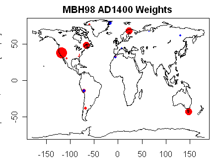
Figure 1. Each dot shows weights of AD1400 MBH98 proxies with area proportional to weight. Major weights are assigned to the NOAMER PC1 (bristlecones), Gaspe, Tornetrask and Tasmania. Issues have arisen in updating each of the first three sites.
Readers also need to keep in mind that two quite distinct principal component operations are carried out in MBH98 – one on gridded temperature data from CRU; and one on tree ring networks from ITRDB and elsewhere. The characteristics of the networks are very different. The gridded temperature networks result in a matrix of data with some effort at geographic organization, while there is no such attempt in the tree ring networks. The tree ring networks are more like the GHCN station networks than like a gridded network. For comparison, imagine a PC calculation on station data in the GHCN network going prior to 1930 with no attempt at geographic organization or balance. Followers of this discussion realize that long station data is overwhelmingly dominated by U.S. (USHCN) station information. Actually, the tree ring networks are even more disparate than GHCN station networks. Many of the tree ring sites are limited by precipitation. Thus, PC on the tree ring networks is more like doing a PC analysis on a pseudo-GHCN network consisting of mostly of precipitation measurements with some blends of temperature and precipitation, with a predominance of stations from the southwest U.S. There are obviously many issues in trying to transpose Preisendorfer methodology developed for very specific circumstances to this sort of information.
Before getting to either of the above larger topics, I wish to lead in with a discussion of the PC calculations in the gridded temperature network – something that hasn’t been on our radar screens very much, but which may shed some light on the thorny tree ring calculations. Here there is some new information since early 2005 – the source code provided to the House Energy and Commerce Committee shows the “Rule N” calculation for gridded temperature networks (though not for tree ring networks) and, in the absence of other information, can help illuminate obscure Mannian calculations.
In the course of this review, I also reconsidered Preisendorfer 1988, Mann’s cited authority for PCA. Preisendorfer (1988), entitled “Principal Component Analysis in Meteorology and Oceanography”, is an interesting and impressive opus, with many interesting by-ways and asides. Preisendorfer is clearly an experienced mathematician and his results are framed in mathematical terms, rather than ad hoc recipes. Many of his comments remain relevant to the present debate, .
Preisendorfer 1988
The underlying model for Preisendorfer’s entire book is a data network obtained from a spatial field over time. His matrices are indexed over time and over space; they are not abstract indexes. He discusses gridded networks of temperature or sea level pressure or composites, but they are never geographically inhomogeneous ragbags, like inhomogeneous collections of site chronologies from ITRDB. Preisendorfer also presumes that the gridded data is produced from the operation of a physical system governed by equations – again something that hardly applies to tree ring neworks with no geographic homogeneity or indexing. The premise of a physical system is intimately related to his use of PCA and methods for retaining PC series:
Various data sets generated by solutions of any of a large class of linear ordinary or of linear partial differential equations exhibit the PCA property in the limit of large sample sizes n. When this is the case, the eigenvectors of the data sets resemble the theoretical orthogonal spatial eigenmodes of the solutions. In this way, “empirical orthogonal functions” arise with definite physical meaning.
As observed previously at CA here , the first step in Preisendorfer’s methodology is “t-centering”, i.e. removing the mean of each time series:
The first step in the PCA of [data set] Z is to center the values z[ t,x] on their averages over the t series… Using these t-centered values z[t,x], we form a new n x p matrix. …
While the purpose of this post is not to discuss short-centering, I’ll note that Preisendorfer explicitly stated that non-centered singular value decompositions of data matrices are not principal components analyses.
If Z in (2.56) is not rendered into t-centered form, then the result is analogous to non-centered covariance matrices and is denoted by S’. The statistical, physical and geometric properties of S’ and S [the covariance matrix] are quite distinct. PCA, by definition, works with variances i.e. squared anomalies about a mean.
This doesn’t mean that one cannot propose some sort of rationale for weights derived from non-centered analyses. However the rationale for such weighting must be demonstrated; in addition, rules derived from Preisendorfer may not readily transpose.
In addition, if the spatial field is scalar and of one type (e.g. only temperature or only sea level pressure), Preisendorfer’s base case uses the covariance matrix. If the data is a composite of two different spatial fields (e.g. one field of temperature, one of sea level pressure), Preisendorfer recommends that the data be standardized by dividing by its standard deviation (page 41).
In his chapter 5, Preisendorfer discusses various rules for deciding how many PCs to retain in a representation of such a gridded system, including rules based on “dominant variance” (such as Rule N). One section of chapter 5 is entitled “Dynamical Origins of the Dominant Variance Selection Rules” and commences:
To provide a simple physical basis for the dominant variance selection rules, we consider the dynamical model (3.12) ….
Retention rules within the Preisendorfer corpus are thus linked to the physical assumptions. The Rule N test is described in Chapter 5 and describes a simulation procedure in which 100 random matrices are generated. For each random matrix, eigenvalues are calculated. The 95th percentile eigenvalue is determined for each eigenvalue and a curve drawn. This is compared to the actual eigenvalues, with data eigenvalues larger than the curve from random eigenvalues being described as “hopefully signal” (p 192).
Necessary but not Sufficient
Preisendorfer himself nowhere asserts that passing Rule N or any other rule demonstrates statistical significance. His entire approach is using PCA as exploratory – something entirely consistent with practice in social sciences. Preisendorfer (269ff):
The null hypothesis of a dominant variance rule [e.g. Rue N] says that the [data matrix] Z is generated by a random process of some specified form, for example a random process that generates equal eigenvalues of the associated scatter matrix S. Hence if one can reject this hypothesis (say via Rule N) then there is reason to believe that Z has been generated by a process unlike that used in the null hypothesis. This rejection does not automatically fix the process generating Z as non-random for there may be alternate random processes generating Z besides that used in the null hypothesis. One may only view the rejeciton of a null hypothesis as an attention getter, a ringing bell that says: you may have a non-random process generating your data set Z. The rejection is a signal to look deeper, to test further.
Preisendorfer goes on to say (270):
There is no royal road to the successful interpretation of selected … principal time series for physical meaning or for clues to the type of physical process underlying the data set Z. The learning process of interpreting [eigenvectors and principal components] is not unlike that of the intern doctor who eventually learns to diagnose a disease from the appearance of the vital signs of his patient. Rule N in this sense is, for example, analogous to the blood pressure reading in medicine. The doctor, observing a significantly high blood pressure, would be remiss if he stops his diagnosis at this point of his patient’s examination.
All of Preisendorfer’s comments on 269-271 are worth considering. He completes the section by describing PCA as a “means rather than an end”:
The novice practitioner of PCA may well fix at the outset the proper place of PCA in his studies of the atmosphere-ocean system: PCA is a probing tool; it is a preliminary testing device; it is a technique to be used at the outset of a search for the physical basis of a data set; it is some initial ground on which to rest diagnoses, model building and predictions. In sum, PCA is not an end in itself but a means toward an end.
Previously Overland and Preisendorfer [1982] had clearly stated that being significant under Rule N was only necessary for significance; they did not argue that it was sufficient. The nuanced approach of Preisendorfer’s actual text is also evident in ecological articles using PCA (articles that are arguably far more relevant to the analyses of tree ring networks than gridded meteorological data.) For example, Franklin et al. [1995] stated:
In the final analysis, the retained components must make good scientific sense (Frane & Hill 1976; Legendre & Legendre 1983; Pielou 1984; Zwick & Velicer 1986; Ludwig & Reynolds 1988; Palmer 1993).
The take-home point here – as so often in these reviews – is that there is no magic formula, including Rule N, by which climate scientists can deduce from principal components applied to a tree ring network that bristlecones measure world temperature or are appropriate to include in an inverse linear regression.
MBH98 on Gridded Temperature Networks
Let’s start by reviewing what MBH98 actually said about their PC analysis of gridded temperature information and compare this procedure to procedures recommended in Preisendorfer (1988):
For each grid-point, the mean was removed, and the series was normalized by its standard deviation. A standardized data matrix T of the data is formed by weighting each grid-point by the cosine of its central latitude to ensure areally proportional contributed variance, and a conventional Principal Component Analysis (PCA) is performed … An objective criterion was used to determine the particular set of eigenvectors which should be used in the calibration as follows. Preisendorfer’s [25] selection rule ‘rule N’ was applied to the multiproxy network to determine the approximate number Neofs of significant independent climate patterns that are resolved by the network, taking into account the spatial correlation within the multiproxy data set..
A couple of points to note here. First the subtraction of the mean of each gridded series is described and is in accordance with the t-centering of Preisendorfer. No short centering here. Although Preisendorfer recommended standardization (division by standard deviation) for series not expressed in common units, he did not explicitly recommend this for spatial fields of one type. To my knowledge, not much turns on this particular decision for gridcell temperatures in terms of final weights for individual proxies; I merely note that this particular step does not appear mandatory or even preferred within the Preisendorfer opus. As noted by von Storch, to accomplish areal proportion, weighting should have been done by the square root of the cosine latitude. Again not much turns on this particular error.
The portion of MBH98 source code archived in summer 2005 in response to a request from the House Energy and Commerce contains the following comments pertaining to the use of Rule N for gridded networks:
now determine suggested number of EOFs in training based on rule N applied to the proxy data alone during the interval t > iproxmin (the minimum year by which each proxy is required to have started, note that default is iproxmin = 1820 if variable proxy network is allowed (latest begin date in network) . We seek the n first eigenvectors whose eigenvalues exceed 1/nproxy’. nproxy’ is the effective climatic spatial degrees of freedom spanned by the proxy network (typically an appropriate estimate is 20-40)
The source code then carries out an SVD on a short-scaled matrix of proxies available in a step (e.g. 22 proxies in the AD1400 step) and calculates the sum of the eigenvalues squared (sumtot) and divides the square of each eigenvalue by the sum of the squared eigenvalues.

If M is the number of proxies in the network (22 in the AD1400 network), the number of retained temperature PCs is set equal to the number of 
So the actual retention criterion (regardless of what is stated in MBH) is based on a rule of thumb related to the number of proxies. The hurdle for significance is that the relative contribution from the eigenvalue exceeds twice the contribution based on equal contributions from all series. I am unaware of this rule of thumb occurring within Preisendorfer 1988 and thus it is not a direct application of Rule N. It seems possible that this rule of thumb can emerge from AR1 red noise models with AR1 values at levels of around 0.3, in the range that Mann likes. So it’s possible that there’s been some sort of offline calculation developing this rule of thumb. I’ll experiment a little with this and report on this today or tomorrow.
As a closing thought, I remind readers once again that, at the end of the day, all that is determined in these Wizard of Oz calculations is the weight that should be applied to individual proxies and, in particular, to bristlecones. Given the NAS Panel statement that strip bark chronologies should be “avoided”, no one should accept the validity of any mechanistic rule supposedly showing the mandatory inclusion of the PC4 (bristlecones in a covariance PC analysis).
I notice that some commenters at Tamino’s claim that discussion of the effect of bristlecones is somehow “moving the goalposts”. For such readers, I refer to our March 2004 submission to Nature where we certainly argued that the MBH principal components method was flawed, but we also focused on the operational impact of the flawed methodology – to overweight the Graybill bristlecone chronologies in the reconstruction – an overweighting that was highly questionable given the prior concerns expressed by specialists over these series.
We do assert, based on the above considerations, that the distinctive hockey-stick shape of the MBH98 temperature reconstruction is primarily due to the Graybill cambial dieback and similar tree ring sites that exhibit non-linear or non temperature-related 20th century growth and to a questionable step in their principal components algorithm that overweights these series. Without these problematic series and without their biased principal component analysis, Mann et al. are not entitled to conclude that the 20th century was uniquely warm based on their data and methods.
The arguments in MM2005 (EE, GRL) are consistent with this. While there’s been a development in some aspects of my understanding of the statistical issues over time, bristlecones have been an issue since March 2004 and are not new goalposts. Since then Mann et al have proposed various strategies purporting to yield similar results to MBH98 (without ever confronting either the failed verification r2 results or the lack of claimed “robustness” to all dendroclimatic indicators). We discussed such salvage proposals in MM2005 (EE), which typically develop different strategies for including a heavy weight to Graybill bristlecone chronologies. Some strategies pertain to policies on PC retention in tree ring networks, which I’ll discuss tomorrow. Typically such strategies sacrifice some important consideration (e.g. geographic balance), but all such strategies with the MBH network require the bristlecones. More on this tomorrow.


60 Comments
BCP Related – over at the CA Forum I have a thread where I am sharing general ecological, meteorological and cryological observations made in areas where Red Fire, Foxtail Pines (and in the future, BCPs) grow. I just returned from Douglas County NV, Alpine County, CA, El Dorado County CA and Amador County CA with new observations. I will link the Forum thread here in a post later today.
So, this is how the number of TPCs is calculated. But how about the selection of TPCs? [1 2 3 5 6 8 11 15] at 1750 and [1 2 3 4 5 7 9 11 15] at 1760 ..
MBH98 explanation:
But this is not true, because selection of [1 2 3 4 5 7 8 9 11 12 13] at 1820 step yields better calibration RE than the one used in MBH98 ([1 2 3 4 5 7 9 11 14 15 16]). Quite an algorithm, anyway 😉
The selection seems to be done offline. There’s an option that permits Mann to state the PCs being used, but how is a particular selection made? It’s a mystery.
Also I haven;t confirmed that this particular method. Note that Mannian short centering concentrates variance in the PC1 in this calculation as well. The loading of variance form a random matrix is sensitive to the autocorrelation in the red noise model as well and this is itself a source of some controversy.
Most of what you posted is a blur to me, Steve, lol. Is a layman’s summary possible?
Abracadbra … alakazam … hockey stick!
JeffA:
I think, in some sense, the lay man’s summary is the map with the dots on it.
Imagine if you calculated the batting average for a baseball team of thee players like this:
Average= (10* Joe + 1* Harry + 0.1* Jane)/(10 + 1 + 0.1)
Clearly, Joe’s average dominates your result. If you told people that you averaged over all three players, that would be deceptive. Yes, you did use Harry and Jane’s averages, but in a way where they have practically no influence on the results.
There are some other nuances having to do with having patched in to estimate Joe, Harry and Jane’s averages, because of incomplete data, and doing a few other things. But, unless you have a very, very good reason to claim that you should weight Joe’s performance more than the others, there is a problem with this sort of weighting.
speaking of proxy dicrepancies, and Mann, Jones, etc. i was searching for time-series glacial photos showing retreat from say 1880 to 1960 (not scary, non AGW) and came upon this IPCC 2001 chapter.
http://www.grida.no/climate/ipcc_tar/wg1/064.htm
fascinating! the last 2 paragraphs are very good along with the graph in pointing out the “unexplained” discrepancies of a possible mid-19th century warming signal. sorry if this is off-topic and if you have covered it before. of course we are coming out of an ice age, but could waldo be hiding in the glaciers prior to AGW?
the map with the dots clearly indicates that unprecedented warming is……regional!!
I would like to ask about Professor Ian Jolliffe, whose book seems to be the definitive guide to the correct use of PCAs. Tamino uses that book to justify the use of non-centred means. In a powerpoint presentation on PCAs “To centre or not to centre, or to perhaps do it twice” Jolliffe appears to say that it is OK to use non-centred means when the data is in the form of anomalies, but that otherwise he does not recommend it.
I do not know whether proxy data from tree rings counts as anomaly data. Can anyone explain whether Jolliffe is behind MBH or not? He is a certainly very highly regarded statistician who is an expert on climatology, does he give the use of non-centred means by MBH his seal of approval?
A technique is neither right or wrong on its own. It needs to be applied to the approrpiate circumstances. Thus, one can’t make the blanket statement “it is OK to use non-centred means when the data is in the form of anomalies” any more than one can say that “concrete is the best building material”. And even then, one can use a ‘good’ technique badly. I have seen many regressions where someone puts a grab bag of variables on the right-hand side, drops all of them with a t-stat below 2 and ends up with a supremely misleading (and invariably lacking in any robustness) model. You can’t blindly follow a recipie with this stuff and expect to get a meaningful result.
#9: Patrick, he does not give an approval to MBH. It is just that certain people try to confuse (by, e.g., using imprecise language) you to think that Jolliffe’s presentation has something to do with MBH-style PCA. Let me try this again:
-Jolliffe’s non-centered PCA means that nothing is removed from the series.
-MBH is not doing non-centered PCA in the sense of Jolliffe. They are removing an estimated mean (average) from the series. Not the whole sample average, but a sample average of a part of series (calibration period). Steve is using the term “short centering” above for this. I used the term partial centering earlier.
Jolliffe states the case for using non-centered PCA (slides 21 & 24):
To put that in the MBH short centering context is essentially to say that if you take long enough tree ring series (say tens of thousands of years) then the mean of that would be the same as the average you calculated over the calibration period (1902-1980), i.e. your “origin”! And this should be true for all of your tree ring series. A reasonable assumption?
Additionally, I’d like to draw your attention to the fact that this Mannian PCA was not described in MBH. They stated that they used “conventional PCA”. So if they truly believed that, for some reasons I can’t imagine, this “PCA” was superior to normal PCA in the situation in hand, why didn’t they even mention it? Why didn’t they tell that for these and these reasons we are not using conventional PCA, but (our own) modification of it? Or more importantly, why nobody has yet to come up with a reference in literature, where this “short centering PCA” is analyzed and/or justified? Or even used besides MBH.
Wow, one need only look at that map and wonder. No data from Africa, one data point in Asia. And to weight tree rings heavily? Sheeesh.
As promised. Here is thread, over at the CA forum, on the topic of possible future studies to correlate ring width and latewood density responses to temperature, and / versus precip (especially cold season snow pack provided moisture) for BCPs and other species found within 100 miles’ radius, at upper treeline, in areas with a reasonably similar synoptic scale and topographical climate:
http://www.climateaudit.org/phpBB3/viewtopic.php?f=5&t=67
Some of the other species of interest may be Red Fir, Jeffry Pine, Foxtail Pine, and possibly even Ponderosa Pine.
Would centering the PCA be like ballancing a hockey stick on the 5 foot snow banks in front of my house?
Re#7, I’ve raised the issue of the “unexplained discrepancies” between glacier retreat and the surface record as stated in the 2001 IPCC TAR before. Gavin at RC responded that ‘he didn’t know why they said that’ and said any discrepancies were ‘overblown.’ I brought the paragraph or two up on Tamino a year or so ago to prove a point, and I was told I couldn’t discuss anything from 2001 since the 2007 IPCC report was out.
One would think that a physical and relatively global suggestion that the surface record is substantially inaccurate at least as recently as 150 yrs ago would be of high importance.
Here’s the major concern about PCA applied to temperature reconstruction that seems to be consistently ignored by virtually everyone.
“The interpretation of the PCs can be di±cult at times. Although they are uncorrelated variables constructed as linear combinations of the original variables, and have some desirable properties, they do not necessarily correspond to meaningful physical quantities.”
This statement can be found in “A survey of dimension reduction techniques” by Imola K. Fodor, available on the Lawrence Livermore Nat’l Labs website, here.
The long and short of it is that principal components are physically meaningless. In order to derive physical meaning from PC’s, they must be interpreted through a physical theory.
Proxy temperature reconstructions are making a scientific assertion, and do not represent an inference restricted to the field of Statistics. Zeroing, normalizing standard deviations, rescaling to and ‘training against’ a time-series temperature measurment does not turn a PC into a physically meaningful temperature trend.
This whole business of blind re-interpretation of tree-ring PC’s, or any other sort of core-derived PC’s, as physically meaningful temperature series absent a physical theory is a scientific grotesquerie. It is no more than false precision, empty of scientific meaning. It is wrong. It is scandalous.
#16 (Pat): I don’t think that’s a problem of PCA in the intended meaning in MBH. They are not giving any meaning to PCs. PCs are treated as if they were other proxies. That is, they are not assumed to be meaningful physical quantities, but only linear in temperature. That assumption is IMHO questionable, but that’s another question. If the original tree rings are linear in temperature, so are PCs as they are simply linear combination of the original series. The actual reconstruction of temperature series out of proxies is suppose to come later in the MBH algorithm (which, of course, does not work out that way).
For the most part I have to agree with Tamino here.
… that it has desirable properties for climate reconstructions… This is true since it produces the hockey stick and this was the desirable property that they wanted.
… that there were good reasons for its selection by MBH…. Also correct since the reason it was selected was because it produces the hockey stick.
re 19
I hope that this is not a distraction but how does Mann select one PC out of several and say it relates to temperature
Jean, #17, as soon as PC1 is scaled to temperature, in MBH and everywhere else, it’s immediately interpreted as representing a physical temperature anomaly. That’s imposing physical meaning by mere assignment. MBH’s argument is in the province of science, not in a province of statistics. As such they are making a claim — superposition of PC1 with a measured temperature converts PC1 into a temperature anomaly — that is entirely unjustified within science. That, no matter that the statistics is rigorous (or not, as M&M have demonstrated).
The first scandal is that a trained physicist, Michael Mann, made such a claim. They second scandal is that it passed peer review and was published. The third scandal is the unholy rush of other trained proxy climatology scientists to embrace a false method — almost certainly because it gave them pseudo-results that revolutionized their field from climatology into thermometry, that in turn granted them fame and tenure. The fourth scandal is that few or no other highly trained physical scientists have called them on it in peer-reviewed print.
I’ve tested my opinion by asking various physicists and statistically savvy mathematicians about the physical meaning of principal components. The uniform answer is that they have none; no physical meaning. Nevertheless, there is no outcry in that field (climatology), or any other, that quantitative physical meaning is being assigned, by mere qualitative inspection, to PC’s from climatological core series.
It’s a terrible scandal; part of the enormous scadalous matrix that is the claim of AGW.
Kristen says ref 14
“Would centering the PCA be like ballancing a hockey stick on the 5 foot snow banks in front of my house?”
LOL May I add in a “howling” wind storm
Re: #4
As a layperson in these matters I attempt to understand the importance of what is being said by looking for things like sensitivity analyses (which in this case goes to the heart of the geographical concentration of data and the performance of the reconstructions depending greatly on the [questionable] use of bristle cone pines); what one finds by reading the fine print of what the authors have referenced and attributed to a reference that might not hold up to closer scruntiny and whether the methodolgies are newly minted or well accepted practices.
Scientists and statisticians do not use the term but one needs to look for any BS — as creatively and imaginatively as it might appear.
I attempted to post this on Pit Bull’s blog, and it was censored. I wonder why?
Dr. Hansen recently gave a presentation at Illinois Wesleyan University, where he attempted to demonstrate that man-made global warming was causing a meltdown in Greenland.
He failed though to mention though that every single long-term GISS record from Greenland shows that the 1930s and 1940s were at least as warm as the present.
http://data.giss.nasa.gov/cgi-bin/gistemp/gistemp_station.py?id=431042500000&data_set=1&num_neighbors=1
http://data.giss.nasa.gov/cgi-bin/gistemp/gistemp_station.py?id=620040630003&data_set=1&num_neighbors=1
http://data.giss.nasa.gov/cgi-bin/gistemp/gistemp_station.py?id=634011520003&data_set=1&num_neighbors=1
http://data.giss.nasa.gov/cgi-bin/gistemp/gistemp_station.py?id=431043600000&data_set=1&num_neighbors=1
#4: Jeff, maybe http://www.climateaudit.org/index.php?p=166 would provide the needed background.
It’s very telling that Tamino fails to link to a single one of our papers, and his cheerleaders and groupies sure haven’t read them. I wonder if Tamino himself has read our E&E05 paper, where we discuss, among other things, the various ways to go between a hockey stick and non-hockey stick reconstruction. One of the ways we discuss is to use centered PCA and vary the list from 2 to 5 PCs in the NOAMER network (see pp 75-76). His post presents it like he discovered it, and we didn’t mention it. We discussed the fact that the hockey stick shape drops to the 4th PC (with accompanying collapse in the associated eigenvalue) in our GRL article as well. He also ignores the problem of insignificance even with 5 PCs, the zero r-squared scores first shown by M&M and then confirmed by Wahl&Ammann, the lack of robustness to excluding the bristlecones, etc.
Tamino claims great insight into why Mann used de-centered PCA in a form that preferentially weights the small number of hockey stick-shaped proxies in the PC1. Yet MBH never stated they were doing non-standard PCA, much less explained to their readers why they were doing it, so his revisionist history is pure speculation.
I guess Tamino also hasn’t inspected the CENSORED folder or grasped the meaning of what was in it. Without the BCP’s the decentering doesn’t matter since the remaining series all have stable means, and no hockey stick emerges in any PC. Decentering mattered once a couple of hockey stick-shaped series were inserted into the network; then the Mann-method mined for the shapes and loaded them into the PC1.
The issue with the hockey stick has always been robustness. Slight changes to the proxy roster overturn the results, slight changes to the method overturn the interpretations, and the test scores do not support the claim of significant extrapolative ability. These things were known in 1998, and if MBH had reported them, their result would have been seen differently from the outset–as a stab at combining some linear estimators, but unable to support any important conclusions.
Ross #26 wrote, “so [Tamino’s] revisionist history is pure speculation.” (underline added)
You’re being far too kind, Ross.
#18
Indeed, MBH99 result corroborates alarmist- AGW theory extremely well. Two natural time-scales (millennial and annual), due to astronomical forcing and weather, and then clearly dominating A-CO2 effect superimposed to those. Designed to kill LTP / 1/f / unit-root models for climate series (Woodward, Grey et al published something related in ’90s., iirc)
I’ve posted on tamino recently. There is a fair amount of boorishness lately – some of it may be because of tamino’s defining himself as Hansen’s Bulldog, and the occasionally intemperate tone he’s adopted. Some because of a mistakenly relaxed moderation policy which encourages the trolls. But it shows signs of improving. The basic explanation of PCA was good, and it was a pity that the MBH material in the last one has been somewhat unfocussed. The result is that it has taken the thread something like 250 sometimes very acerbic comments to get to the bottom of MBH style PCA.
Me included, by the way. I wouldn’t have got to it properly without having gone through Tamino’s defence and feeling that this surely could not be right. Another good thing that has come out of it is that some people are now using R and posting results. The end result may be to improve the quality of discussion on his blog greatly, even if he should eventually agree he was mistaken about MBH’s PCA.
It would be a good thing if so. Tamino has a real talent for education. He can take something complicated and confusing and explain the main lines of it very clearly, as one has seen both in the PCA postings and some others. One hopes he’ll moderate and make commenters do so, as he says he will.
The striking thing about the blog in this episode has been social. There has been a claque with a very strong party line. It is not all commenters, but its a substantial number. Among them, the validity of MBH and the HS are articles of faith. To doubt them is to be a denier. It is logically perfectly possible to think MBH wrong but AGW a true and important thesis. The claque even admits this, and keeps saying that the validity of MBH does not matter, so we should all move on. At the same time, they react with complete fury to any questioning of it. The only place I’ve ever come across this insistence on defending to the death issues which are simultaneously contended not to be central to the main argument is in rather extreme and fundamentalist political and religious sects. One could perfectly consistently have believed that the Katyn massacre was done by out of control Russians, and that the Russian regime was an example for humanity, just not perfect in this instance. But no-one in the Party was able to do that.
In fact, simply to enquire about the exact nature of the IPCC account, without any suggestion of scepticism, will result in being called a denier by some posters. I have been accused of being a denier for pointing out that if the climate sensitivity to CO2 doubling is 4 degrees, 1.2 is due to the direct effects of CO2 and the laws of physics, but 2.8 is due to complex positive feedback mechanisms.
It is striking that some of the more egregious examples of denialism occur in the ranks of the faithful, who spend so much of their energy accusing enquirers of it!
However, its not all negative. One of the posters is recently reading the M&M material and reproducing the arguments using R. Whether he turns out to agree or not, this will be improve the blog.
Personally by the way, I don’t know about warming. I know I do not believe in decentered or whatever it is PCA. I’m not convinced by high numbers on CO2 sensitivity either, they really don’t seem evidence based. But I can’t see it is sensible to cheerfully make large changes to the atmosphere and just not worry about it.
I think its telling that despite such clear multiple independent demolitions of the Hockey Stick, climate alarmists cannot let go of the Hockey Stick – because it clearly shows in graphical form that which they believe to be true about the world.
The one characteristic which encapuslates that belief is the fact that the Hockey Stick appears to follow the carbon dioxide Siple Curve. Thus it demonstrates a belief in greenhouse warming, whatever the ice core records may say.
Its not that Steve and Ross’ criticism has been shown to be even slightly mistaken – its more to do with the will to believe something that the scientific method says should be rejected.
In Tamino’s and I would say Dr Quiggin’s ham-handed interpretations of your work (RC is deliberately omitted as a COI in the social network), what was the rough timeline of event discovery for the sum points by which M&M has been you’ve critical the HS?
1) Decentered PC’s
2) Noise mishandling
3) Proxy selection and bias
4) Misuse of Preisendorfer
5) CE vs. other correlation coef’s
6) The hidden BCP proxy directory
7) General BCP misuse as temp proxies
8) Others
The chronology of 3-7 would be of particular interest?
Correction: … timeline of event discovery for the sum points by which M&M has been critical of the HS?
Re #9
I asked Dr Jolliffe if he endorsed Mann’s non-centred PCA and this was his email reply on 25 Feb 2005
I find it very interesting that the proxies that show warming are assigned much more weight than the proxies that show cooling.
Does anyone know the justification for this weighting?
Steve, slightly off topic, but now that you have the link to the source code (my Fortran reading is lousy). This may be old news to you, but I don’t recall it mentioned anywhere:
Me and UC were fine tuning our MBH emulators a while back. One of the annoying discrepancies was that we were getting lower verification REs than reported although our emulations otherwise seems very good. Even WA seems to have run to the same problem; they even have one hand-waving appendix for the issue (Appendix 4). Well, I think we found the reason (can anyone confirm this from the source code?): it seems that Mann is calculating verification REs with respect to “sparse” reconstructions! That is, verification REs are not calculated from the actual (stepwise) reconstructions, but from NH stepwise reconstructions obtained by limiting reconstruction grid cells to those used for calculating the sparse instrumental temperature.
Steve: Yes, this is what he says he does. I have code to extract the “sparse” dataset.
Re# 30, John,
You are right to point to the “marketing appeal” of the hockey stick but it is also the lynch pin of IPCC, 2001, which Tamino thinks we should now forget. See IPCC, 2001 WGI Chapter 12 (Attribution) page 702:
We shouldn’t get into conspiracy theories or too much social network analysis but note who were the lead authors of that chapter and of the Palaeo Chapter it was referring to and then remember who were the Review Editors of IPCC, 2007 WGI Chapter 6.
Steve, beautiful work. Please keep hammering this.
Suppose that tree rings in carefully controlled conditions did serve as a good guide to air temperature. Then go out to Nature like you did, to find that sometimes the air was cold from the North and then warm from the South. Lacking fine detail of winds, one is not allowed to assume that a PCA over decades will unravel useful predictive ability linking temp to tree rings. The calibration period will lack essential data and the PCA, done conventionally, will not indicate a comprehensible outcome.
Dreamin’.
The irony is that such a flat climate in the past is kind of an argument for a low climate sensitivity…
Tamino and RC must know this. They seem to cling to the HS becuase it is effective propaganda.
David Holland #37, 4.34
Thank you very much for that quote from Professor Ian Jolliffe.
We can certainly see what he thinks about MBH from the quote: “I came to conclusion that I simply could not understand what was being done sufficiently well to judge whether Mann’s methodology was sound, but I certainly would not endorse it.” I cannot believe that Bulldog would have used Jolliffe’s book as an authority if he had been aware of that comment.
It is a little surprising that someone like him who is clearly an expert statistician specialising in Climatology who has written very important works on PCAs and (weather) Forecast Verification does not have more curiosity about the methods used in MBH98, especially since his text book is used on Real Climate and Bulldog to justify them.
A bit OT but,
In #28 I referred to [1], where they write:
And they say that it might not be reasonable to forecast the future temperatures as increasing (based on the data only). This was published in 1995, and few more cold months (say zero anomaly for HadCRU for the rest of the year) , and 1996 – 2008 monthly anomaly will trend down.. (That wouldn’t change anything, just a note)
[1] Selecting a Model for Detecting the Presence of a Trend, Wayne A. Woodward and H.L. Gray, Journal of Climate, Aug 1995
I’m sure he wasn’t aware of that comment, but would that really stop him? All he has to do is convince his readers that Jolliffe supports MBH98 methodology. Looking at many of the responses on that thread, he has. They aren’t going to come over here and see Jolliffe’s comment. Tamino’s not going to let it get posted on his site.
When thinking about Tamino’s attempt to present PCA on decentered data as some kind of legitimate methodological innovation, two points stand out:
– The source he cites is a powerpoint slide show on a tangential topic, from someone who has said he does not endorse the particular method in question;
– de-centering on a subsample merely inflates the variance of vectors whose means shift over that subsample. Since the choice of subsample interval is arbitrary, the relative inflation of variances is arbitrary. That’s why PCA on centered data is standard, and departure from the standard requires explicit disclosure and justification. If the results depend on the particular form of decentering you have to explain this and make a case why the arbitrary transformation of the data is necessary. You could make a case for picking the earliest period for centering, and then the series that get boosted to the PC1 would be those with a trend in the 1400s. That wouldn’t “prove” that those series are the most representative of the global climate though.
You make a very good point which should not be overlooked. In his book, Jolloffe allows (grudgingly, IMHO) that a case might be made to centre at “the origin” if the origin is a meaningful value:
The italics were not added by me but appear in the text. The entire section appears to be more of a matter-of-fact exposition of what is done by climate scientists than an advocacy of the correctness of the technique. It seems pretty clear from the italics that the centering be in respect to a fixed value and not an arbitrary value estimnated from the sample. As you correctly indicate, the latter would greatly increase the uncertainty of any results.
As a matter of note, his treatment of the procedure in the powerpoint (the lack of interpretability of the second “component” in his example and the warnings regarding its use in the final slide ) seem to clearly indicate his understanding that this is a questionable process.
Re: #33
I think I should have added to my list of layperson’s methods of evaluation of statistically and scientifically technical papers, the opaqueness factor as noted above and the suspicion and/or blatant use of cherry picking data inputs, or outputs, for that matter. Cherry picking can sometimes be revealed in the sensitivity analysis I noted earlier, but sometimes it obvious without analysis. It all goes along with looking for the B word tendencies.
I have aired this view previously but, in my mind Mann’s magnum opus gave the climate scientists a measure of past climate that fit their already formed consensus view so well that it was difficult for any but a few climate scientists to deconstruct what was done. It would appear that climate science has moved on to preferentially using climate models over climate reconstructions, but there are many climate science supporters (and a few scientists who are hardcore Mann supporters) of the consensus view that evidently do not have sufficient conviction of their views to allow for the Mannian mistakes.
Therein lies the problem. Incorrect centering inflates the variances with a DC bias, placing emphasis on proxies that have time varying means. Those that have stable means, near the chosen center point, will be unaffected. A similar problem arises with Mann’s ergodicity assumption in his RegEM method. Not that he explicitly assumed ergodicity, but his method for taking the mean of the means and applying it to the entire block does just that. Jean S first noticed this.
Mark
re 32. see if you can get that posted in tammy town
Mark,
Ah, another accident. BTW, any guesses why Rutherford et al. 05 shows only 1400-present reconstructions ?
I wouldn’t doubt if it were actually an accident, though a good scientist would strive to learn the problems with such assumptions (explicit or implicit), and correct any errors that may have resulted in previous analyses.
Perhaps the DC bias prior to 1400, such as during the MWP, which coincidentally shows up in most of the proxies (as I recall), would cause problems for the “warmest in a milluuuuun years” claim? 🙂
Mark
In the work that I do with survey data, I am always nervous when using PCA to identify a more efficient way to summarize the data that what I am finding are groups of respondents not groups of related explanatory variables. The only way to really tell, as Steve points out above, is to carefully check that the variables loading on a particular factor make real sense and do not reflect some as yet unmeasured variable that links a subset of respondents. This inspection has to be done factor by factor.
My read of what Steve and Ross (and others here) have done is point out that PC1 or the HS factor is a characteristic of group of respondents (the BCPs) and not the underlying temperature signal.
Is this a correct interpretation?
Thanks Lucia! I was kind of thinking that’s where it was headed, but wasn’t sure.
Thanks Ross!
If you amend that to may not be the underlying temperature signal then yes, your interpretation is correct. This is confounded by the fact that the HS signal is predominantly present in BCPs, which end up getting weighted heavier than other proxies. Whether or not it is truly temperature is hard to say without removing other factors that may be contributing to their shape, too. PCA does not assign a “flag” to the results indicating which is which, and when multiple inputs to the system (e.g. solar, precipitation, CO2 fertilization) are correlated, disaggregation is even more difficult (if not outright impossible).
The short answer is that the “signal” that shows up is assumed to be temperature simply because the surface temperature readings are increasing at the same time, and the BCPs are assumed to be responding to temperature, not other factors. That BCPs will necessarily respond to local temperatures, not global temperatures, is lost on the proponents of the proxy reconstruction theory (via PCA), btw.
Mark
If I were a mathematician, I would say the lack of a gridded data set representing a physical system governed by equations that can be analytically solved invalidates the entire use of PCA methodology in the analysis of any climate data. Mathematicians are sticklers for proper use of methods, and rightly so. They are the “grammar” [enforcers] of the scientific world.
The reasoning is simple. You have no gridded surface data for temperature or rainfall or any weather phenomena, you have scattered stations around the globe and nearly nothing on the ocean. With satellite data you at least have a grid, but the physicist in me says good luck finding an equation that can represent the physical reality you’re collecting data from. In too-simple terms, no boundary conditions = no understanding of what’s going on.
What Jeremy said.
In a way, this should never have got to the point of statistics, except to probe for their applicability.
In # 36 above I mentioned that temperature of trees and wind direction confounded. The tree is a living system with cycles of growth and rest that are impacted by temperature. There are times when a short blast of hot or cold out of season can limit or help growth for a year or more.
Analogy: People need to drink water to avoid getting ill/dying. Over a month, one might drink a similar volume each day; or to argue by extreme, could drink at twice this rate in the first fortnight and drink nothing in last fortnight. Monthly average remains the same, conseqence is reduced growth, maybe permanently.
Same with trees. Growth is affected not just by the average value of monthly temperature, but also by the distribution pattern of temperatures within each month. If the calibration period cannot infill the fine structure, the stats will not be capable of reconstructing the past.
Having taken very rare trees from China to Australia, I know a little about coping wih seasonal changes (NH to SH in a day), so my comment contains practical as well as theory. Is that so novel?
re: 30
5) RE vs. other correlation coef’s such as R2 (CE wasn’t determined and therefore not an issue)
I’m confused (not difficult!), and not being a statistician is not helping…
There is much talk of the bristlecones being overweighted, that I understand & hence the reason the hockey stick appears – what I don’t quite get is how the weightings get to be where they are. Is it a deliberate choice by Mann et al, or is it some artifact of PCA analysis which up-weights certain datasets “automagically”?
(Apologies if this is a dumb question, or is answered elsewhere)
<
#56. The problems are multi-layered. No one knows for sure what Mann knew about his method. There are issues relating to the application of correct PC methods to tree ring data sets. These problems are made worse by the erroneous Mannian method.
With 20-20 hindsight, it would have been possible for Mann to have used a PC method which was less bad – in which case the issue would be squarely on the validity of applying conventional principal components to the North American tree ring data set as a means of obtaining a temperature proxy – which has never been established – and of the validity of bristlecones.
Think of a murder victim with multiple stab wounds. The police arrest the husband and can prove that he stabbed his wife repeatedly and charge him with murdering his wife by stabbing her to death. Let’s now suppose that his defence is that he had already smothered his wife to death and the stabbing took place into her dead body so the claim that he murdered her by stabbing her to death was wrong. As I understand it, the count could be amended and the accused would not go free on such a technicality.
Mann applied PC methodology applied to a tree ring network with multiple bristlecones. Trying to find the “real” problem in such a mess is like a complicate episode in CSI. The bristlecones are one problem; applying ordinary PCA to tree ring networks is another problem; Mannian PCA is another problem. Removing bristlecones from this nbetwork doesn’t necessarily improve things at all. I’m not saying that there’s a “right” way to get an answer out of this mess.
Preisendorfer 1988
Tree ring response to temperature can hardly be described as “linear”. I would think “parabolic” is more apt…. The pretext for using Preisendorfer seems to collapse from the outset.
#57: Thanks Steve, I guess until Mann actually comes clean about exactly what data & methods he used, we shall never know….
Mark T
Or lack of long-term cooling trend might be the reason, who knows 😉