Standardization in Mannian algorithms is always a bit of an adventure. The bias towards bristlecones and HS-shaped series from the impact of Mann’s short segment standardization on his tree ring PCs has been widely publicized. Smerdon’s demonstration of defects in Rutherford et al 2005, Mann et al 2005 and Mann et al 2007 all relate to errors introduced by inconsistencies between the standardization methods and the assumptions of the algorithm. Jean S has pointed out further defects that have not yet been incorporated in the PRL.
Jeff Id and I have been exchanging digital files. Jeff has provided some intermediates from his Matlab run and I’ve made some progress in emulating this in R. I think that I’ve got a stable emulation of the Truncated TLS operation (Tapio Schneider’s pttls function) and I’ve got a pretty close emulation of the Xmis object in the first step of the RegEM operation and am getting close to the first step X object.
Along the way, I noticed something which may prove of interest – tho I caution that this is just a diarized note for follow up at present.
One of the fundamental assumptions of Tapio Schneider RegEM is data is missing at random. This is clearly untrue for Steig’s data. However, this sort of failure doesn’t necessarily mean the algorithm is worthless – but careful authors would surely have discussed this issue and its potential impact.
One of the key non-randomness is that some series are missing a LOT more data than other series. It looks like this could have a material effect on weights through an interesting step in the algorithm.
Schneider’s algorithm first centers the data (Matlab code below):
[X, M] = center(X); % center data to mean zero
Then missing data is set at 0.
X(indmis) = zeros(nmis, 1); % fill missing entries with zeros
A little further on, the series are divided by their standard deviations:
% scale variables to unit variance
Do you see what happens? If a series has a LOT of missing data, the missing data is all set at 0 for the purposes of the standard deviation. Could a potential bias arise? Here’s a plot of the standard deviation after first step infilling. It’s interesting that the infilled standard deviations of inland stations are so much lower than coastal stations, though there’s no reason to believe that this is the case physically. It’s only because the inland stations are missing more data – which is thus set to zero and reduces the standard deviation. This might reduce the weighting of the inland stations relative to the Peninsula stations if it persists through later steps. I don’t see any code right now that would appear to compensate for this (but I haven’t finished yet.) There’s no reason why there would be such code. Schneider assumes that data is missing at random, while Steig and Mann ignore this caveat. I’ll keep you posted as I continue to work through my emulation of Schneider’s RegEM.

UPDATE Feb 17:
Here’s the same plot after step 21 which is fairly close to convergence. The variations in std dev still appear unphysical.

UPDATE Feb 19:
Tapio Schneider says above:
The initial variance estimate is biased because missing values are set to the mean (zero after centering), but the estimate is iteratively improved. (One can show that the estimate in the ordinary EM algorithm converges monotonically to the maximum likelihood estimate for normal data; in the regularized EM algorithm, this monotonic convergence is assured for a fixed regularization parameter but not necessarily in general, when regularization parameters are chosen adaptively.)
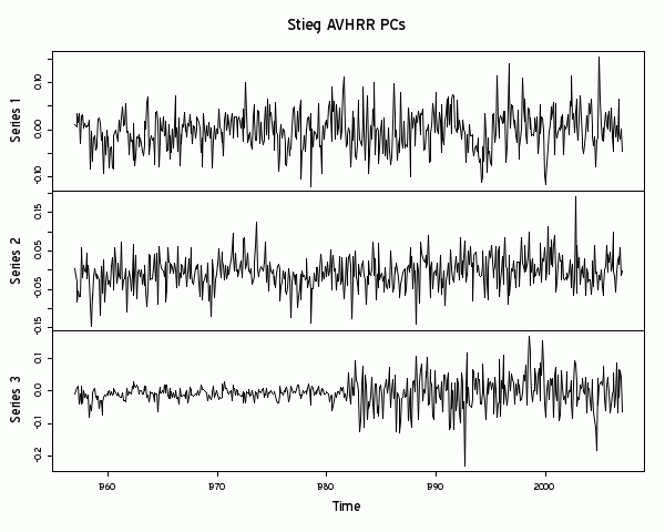
The following diagram of PCs is from the AVHRR data. Note the structure of the PC3. PCs recover patterns. The pattern being recovered in the PC3 is surely the infilling of data with zeros.
So notwithstanding Tapio’s comment, it sure looks like the infilling with zero pattern is preserved in the final result. As a caveat, while Steig said loudly that he used the unadorned Schneider algorithm, this statement contradicts a statement in the article that they used the algorithm as “adapted” by Mann and Rutherford. Previous adaptations by these authors have been criticized by Smerdon in three publications and it is possible that the phenomenon observed here is related to the adaptations rather than the Schneider algorithm itself. Without knowing what Steig really did – and he’s incommunicado – there’s still a lot of speculation here.


91 Comments
Very interesting —
Does applying RegEM to the surface+AWS data in fact seem to be as straightforward as Steig and Gavin have claimed? (Ie just fill a matrix in an obvious way and call Schneider’s subroutines.) How about the TIR+surface data?
Does CA have a page with the surface, AWS, and TIR data in single files?
Steve: surface, AWS are collated at CA/data/steig in Data.tab as Data$aws and Data$surface. The TIR data is presently unavailable as used in Steig. Its only available unprocessed for clouds on different grids and time scales.
Re: Hu McCulloch (#1),
Hu – yes it is that simple, at least for the AWS reconstruction. Jeff Id’s version doesn’t exactly match Steig’s but it is very close. There may be some differences in how Steig rounds or calculates anomalies prior to putting the data in RegEM.
This makes me think there is a different methodology for the satellite recon as it is composed of 5509 gridcells. If you dumped 5551 data series into RegEM (5509 + 42 surface), presumably the 42 would have a very small impact as RegEM doesn’t know which is which.
Steve your observation about the amount of missing data affecting weighting is interesting. When I was working with my gridcell version, I noticed that averaging data series significantly decreased the number of missing data points in the resulting series (makes sense). This may be important as my derived interior cells had very few missing data points since they were averages of neighboring cells. This may have increased their overall weighting.
Steve:
I am not sure that I would say that the smaller stdev are “inland” as much as non-randomly distributed. This approach of substituting “0” also seems counter-intuitive: More missing data ==> lower stdev?
Re: bernie (#2),
Seems pretty straight-forward to me. If you have a bunch of people about the same height and then a couple of outliers and then someone tells you “here’s another 100 people of the same exact height as the average, you’d expect the StD of the 200 to be less than the 100, wouldn’t you? 0 is by construction the average of the data after Schneider’s first step, so infilling more 0s would decrease the StD. Of course, the fact that it’s simple and easy to understand doesn’t make it right.
Re: Dave Dardinger (#15), no.
If you have a population with mean zero and standard deviation 1 and calculate the mean and standard deviation from a sample of size 200 you will get sample estimates very close to zero and 1. If, however, you take a sample of size 100 and add 100 zeros you will get a mean of zero and a standard deviation of 1/sqrt(2).
A clear reduction in variance relative to the true population variance.
That’s what it looks like to me. I’ll see if the Jeffs agree.
I ‘d rather stick with back-of-envelope calculations, then.
You misunderstand … Clearly, lack of information means less uncertainty because the more we know the more we realize what we don’t know. Therefore, perfect ignorance means perfect certainty. The best data series is one that consists entirely of missing values because then there is no variability to confuse us.
If the above does not makes sense, that’s because it does not.
*Aaarrrgghhh!!!!***
— Sinan
Re: Sinan Unur (#6),
Until you have to divide by zero.
Re: Kenneth Fritsch (#23),
In which case the appropriate correction would be applied.
I am going to stop now to allow Steve to do the real work as usual. I hope it is obvious that both my comments are sarcastic observations.
#1, 5. The algorithm is relatively simple, but the “infilling” concept is a pernicious metaphor in some applications. They “infill” medieval temperatures based on bristlecone pines.
De facto, there’s a kind of regression relationship buried in the algebra. MBH also had this sort of bristling algebra, but ultimately there were huge cancellations and much of it could be reduced to a few lines.
At some point, there’s an implicit regression relationship between the old stations and the new AWS stations that’s used to extend the new stations. It’s not unreasonable to cross examine these for biases.
Substituting the mean of the variable for the missing value is standard for the EM (without the Reg) procedure which is used when there are relatively few missing values where the value is missing at random.
When I was looking at the satellite reconstruction earlier, I noticed that the reconstructions seemed to be less wiggly before 1982 than after. I detrended the sequences (separately for each period) and calculate the variances of each sequence before and after 1982 using the script
with a histogram of the ratios looking like
(Hmm… on my screen it looks like there are gaps in the histogram in the upper end, but they aren’t really there.)
Notice that the largest ratio is .894. The sequences are all considerably less variable in the time period when there were no satellite observations, a serious underestimation of the variability of the reconstruction.
The same is true for the monthly mean sequence. A side effect of this is that small slopes will reach “significance” with fewer observations because the MSE of the regression is underestimated.
Re: RomanM (#8),
“… on my screen it looks like there are gaps in the histogram in the upper end, but they aren’t really there.”
With MS Internet Explorer I see the gaps, but they go away if you magnify to 110%. That seems to happen with a lot of graphics here.
I don’t see the gaps with Google Chrome.
Re: Steve Reynolds (#32),
I didn’t know what he was referring to. There were no gaps at work but now I see em. It was confusing.
Re: RomanM (#8),
Roman, (minor point) you are trying to fit more than 1024 vertical lines exactly onto a screen 1024 dots wide (or whatever the specs are). Some of the lines with fractional pixels fall between stools and disappear. An inelegant solution is to rotate your graph 0.2 degrees or so under graphics before posting. But this makes digitising harder after the event.
Re #1,
I’m having trouble opening Data.tab with Internet Explorer, Excel, or Notepad. Is it specific to R?
Steve: yes. sorry bout that. I’ll ASCII it if you want.
A few tips for those who may be trying to run this themselves in Matlab…
Steve’s Data$surface in Data.tab contains 44 surface series. In the SI, Steig says only 42 of the series are used. Two stations aren’t used (Gough and Marion) due to their high latitude. Make sure you remove these series or the recon doesn’t match Steig as well. They are columns 17 and 26 in Data$Surface. The temperature data also needs to be converted to anomalies.
Here is the Matlab script Jeff has been using, it’s simple (fix the path of course):
See Jeff’s website for the discussion as to why the options are set these values. Descriptions of the options are found in Steve’s link to Schneider’s algorithm above.
I had an idea a few minutes ago, I’m not sure if it makes sense. What if they took the 3 sat TIR pc’s and put those in RegEM instead of the full data to create the pre satellite trend? That would explain Roman’s histogram results above and would address the overwhelming data of the full gridded matrix compared to surface stations. Since RegEM uses the same 3 PC’s I’m guessing it would mathematically work for infilling that way.
A lot of guessing but why not.
Re: Jeff Id (#11),
I don’t think so. I taught EM several times over the past few years in a multivariate course. The difference between that and RegEM is the use of an exotic method of relating the infills to the observed values.
The RegEM method would infill a relatively smaller number of missing and/or deleted values in the 1982 to 2006 interval, but the relationship between the manned stations and the satellite values would be determined by mainly observed values. These values include natural variability. The time interval which had no satellite observations was infilled by a method which uses the expected value of the observation given the observed values at that time point (only the stations) using the relationship determined from the time when both satellite and station values are present. This will naturally produce much lower variability infills.
What I still find strange is that Steig then replaced the observed satellite data with the PC reconstructed values (which would also be of lower variability than the observed). Maybe that was needed to produce a “significant” result…
I do not know the data well enough, but if there are several periods when post of the data stations were overlapped and operational (not buried), then surely these cound be identified and variances calculated on fairly full data sets. They might be too sparse to lead to a smooth teconstruction of the temperature graph over the years, but they would set a limit for the variance so that artificual estimates could be identified.
In a study I’ve just done of the the “best rural” stations in Australia for the last 40 years, most with complete data, the standard deviation of the average annual temperature derived from daily temperatures ranges from
SD: Tmax High 0.81 Tmin 0.86
SD: Tmin Low 0.34 Tmin 0.31
The average temperatures are about 30 deg to 20 degrees.
The site position (coastal or inland) has the main correlation with the SD value.
Re: Geoff Sherrington (#12),
My post was hurried and I will clarify. The purpose is to give a range of SDs and means of temperatures from Australia over the last 41 years, for data with essentially no infilling.
Three stations suffice.
Giles, lat -25.0341, long 128.3010. Far inland.
Digression: I took a whole year at random, 2006. The daily observations gave
T max: Mean, 29.66, SD 7.17
T min: Mean 16.23, SD 7.23. I have reservations about using annual averages of these days in the next section as they are not reflective of the daily variation by simple arithmetic average.
Giles annual, 1968-2008 41 years.
T max : Mean 29.3, SD 0.82. Linear best fit slope 0.019 deg C/year. (HIGH SD).
T min : Mean 15.8, SD 0.75. Linear fit 0,024 deg/year. (HIGH SD)
Site is warming abnormally fast, adding to high SD.
Broome, lat -17.95, long 122.22. Coastal.
T max : Mean 32.1, SD 0.534. Linear fit -0.0002 (No temp change. LOW SD)(Where has Global warming gone?)
T min : Mean 21.1, SD 0.71. Linear fit 0.0033. (Slight temp change. HIGH SD).
Illustrates that SD can be higher for Tmin than Tmax dataset.
HIGH SD and LOW SD are terms relative to the whole dataset of 17 stations. The lowest mainland SD was 0.31.
Macquarie Island lat -54.48, long 158-95. Isolated, on the way to Antarctica.
T max : Mean 6.69, SD 0.35. Linear slope -0.0032 (Where has global warming gone?)
T min : Mean 3.14, SD 0.37. Linear slope 0.00015 deg/year. (Where has global warming gone?)
In the context of this thread, if Antarctic satellites can estimate surface snow temperatures and their SDs when cloudless, what SD can be assumed when inferring under-cloud temperatures? (See Broome example).
Further comment:
Re: MJT (#14),
In reference 2 (2006) there is a statement about in-filling:
I strongly disagree with this. You cannot guess or interpolate a missing value and then state that you have improved accuracy, because you have no missing value against which to measure accuracy. It is a tool of convenience, but it is not science.
Later these authors add, with a figure that –
Does anyone have an explanation about methods for adding “texture” to graphs so that in-filling looks more normal? I refer in particular to the appearance of projections that seem to splice neatly from where the actuals leave off, as if there is some way to know when future climate patterns will happen. To me, if you infill data, you should leave a straight or near-straight dotted line and an explanation in BOLD.
Re: Geoff Sherrington (#46),
In other words, the filled in values are more accurate than the measured data. Have any of these guys even seen the inside of a lab or been out in the field in last twenty years?
Re: Jeff C. (#47),
Dr. Steig is currently on site in Antarctica, presumably gathering data which, via RegEM, Mann can be use to update the Graybill chronologies.
Re: jeez (#48),
Understood. The quote was actually from algorithm authors, not Dr. Steig. I was probabaly a bit too snarky, but it sounded like the authors were blaming the differences between real measurements and modeled values on noise in the measurement. My background is Systems Integration and Verification. We spend a fortune on testing to verify the models, not the other way around.
Re: Geoff Sherrington (#44),
That statement also had me wondering but I linked the paper because it specifically tries to address the issues with regEM in regards to data infilling and also gives a good overview of other methods of infilling in the introduction. The salient point to me being that if your data set is non-gaussian and non-random then regEM is not well suited as a method for infilling.
Steve stated that the non-randomness of this data doesn’t necessarily mean the algorithm is worthless but given the statements of Scneider himself and those implied in Kondrashov and Ghil (2006), at what point can you rule out RegEM being used on a particular data set to produce pertinant results? IE are there Gaussian/Randomness standards used to disqualify data sets in regards to RegEM? I have no background in statistics though so maybe I’m asking the wrong questions.
Re: MJT (#52), the deal-breaker would be any reasonable expectation that the reason certain observation missing had something to do with the value of that observation.
You can visualize this fairly easily. Take any photo. Delete 50% of all pixels (randomly and independently — that is, toss a coin for each pixel, and delete it if the outcome is tails) and replace them with transparency.
Any reasonable gap filling algorithm that uses the non-deleted information efficiently would do an OK job of getting back an image that is similar to the original.
Now, go ahead and delete the same number of pixels in the middle of the image. There is no algorithm that can give you back what was there.
The difference: In the first case, whether a pixel was deleted did not have anything to do with where the pixel was. In the second case, there was a systematic relationship.
There are cases where a systematic reason for the information to be missing does not pose such a problem. For example, if you deleted every other pixel, instead of doing away with a large block in the center, these algorithms would probably be OK.
Even when an algorithm does a good job of producing something close to the original information, it is obvious that the infilled image contains less information and this needs to be taken into account.
— Sinan
Re: Sinan Unur (#53), Thanks for the reply Sinan, and that certainly makes sense. If there is a non-random, ie gaping hole in the center of the picture, I could readily assume that regEM would not accurately infill the data. I guess the question is, is there a test of the data, besides the obvious visual one, that would qualify the miss data to sufficient randomness to be able to use regEM? Specifically is there a statistical test that does this for both the spatial and temporal data?
To further expand on your example, assume that the picture you are referring to is one of a set of frames in a movie that is missing pixels(data). Also what you are trying to determine and infill for each frame is the brightness of each pixel. How do you determine if the data contains enough randomness, both spatially and temporally, to establish a trendline of the brightness of the overall movie using regEM? I guess the same question would apply to the gaussianity(word?) of the data. Perhaps there isn’t a specific test or statistical qualifier to rule a data set in or out for RegEM and maybe I’m just trying to oversimplify the issue. From my reading of the various posts though, it seems the data fails the simple, “hey theres a hole in the middle of the picture” test.
BTW great site Steve, thanks for all the effort you and the others put in to make sense of AGW world.
Mike
Re: MJT (#57), missing means missing. I.e., one must come up with a justification other than the information contained in the non-missing observations to convince oneself that missing values are independent of what is being observed.
So, in this case one has to look at why each and every one of the observations is missing. That is, whether a specific measurement is missing must be independent of the temperature.
— Sinan
Re #9,
Thanks! That would be handy.
Re Jeff C #10,
How did Steig (or you) compute the “anomalies”? Computing anomalies consistently is a problem when there are big periods of non-overlap (as I guess is the case with even the surface stations). Doing it wrong could easily mask or exaggerate trends.
A further complication is that there are strong seasonals, so a different “norm” needs to be computed for each month, and the months are not evenly represented in the data that are present.
Was the “combined anomalies” file provided by Steig?
Re: Hu McCulloch (#13),
Yes, I think that may be one of the reasons why the Jeff Id reconstruction doesn’t exactly match Steigs. I don’t mean to speak too much for the other Jeff, as the combined anomalies file was generated by his code. I think he calculated the row means excluding those missing data and then subtracted the means from each value.
The code is below. Jeff Id – can you clarify this?
Re: Jeff C. (#16),
some differences will definitely be thrown up because Steig’s standardization excludes Dec 2002 and later – as Nic L has shown.
For now, I’m working with a Dec 2006 end point as in the above script, but we’ll need to end in Nov 2002 to be file compatible with Steig.
Re: Steve McIntyre (#21),
As per my posts on the Carnage thread, quality controlled data from Wisconsin-Madison (covering the bulk of the AWS) only became available for December 2002 last October, and is still mainly unavailable for January 2003 through January 2007 – one can see on the READER pages how little data during this period appears in black. However, in many cases there was sufficient data availability (>90%) for data to be shown in green and included in the text files. For December 2002, most of the original data had <90% availability and so was shown in red and not included in the text files. When the QCed data December 2002 became available last October many data points were added in the AWS READER text files. Further changes to the text files were made in December 2008 when some later QCed data for Ferrel and Marble Point became available. It is only where changes were made to the READER text files between Steig downloading them and Steve archiving them that adjustments are needed to Steve’s data in order to reproduce Steig’s results. Most of the post December 2002 AWS data has remained unchanged. Some differences, of unknown origin, also exist in the pre December 2002 data between Steve’s archived copy and what Steig seems to have used. There also appear to be anomolies in Steig’s calculations of mean monthly temperatures for some AWS.
Re: Jeff C. (#16),
The code takes a monthly average into vector ‘an’ and subtracts from the individual temp stations. I think this is an issue in the reconstruction but I also suspect data version problems or the inclusion of a station which shouldn’t be. I haven’t gone through the individual series just yet to check versions. This is what Jeff C caught that helped improve my initial run’s until it was at least usable.
Re: Jeff Id (#27),
Jeff – I think the data versions and stations to be included are straightened out. I’m sure we have the 42 surface stations correct. Regarding the AWS stations and the changes, we are using Steve’s Data.tab file that was from the BAS scrape on Superbowl Sunday. This was before any of Gavin’s mischief and the subsequent changes to the READER data set. As long as we continue to use data.tab to compare to Steig’s original reconstruction we should be okay.
I think Steve and Ryan’s observations regarding the anomaly calculation window closing in 2002 may help narrow the gap between your recon and Steig’s. I’ll pursue this and see what happens.
Re: Jeff C. (#16), the comment in Jeff Id’s code:
reflects the fact that these are in fact the SAME station – in fact I believe an AWS, so I think Steig is wrong when he claims that no AWS data was used in the main reconstruction. I couldn’t say whether treating this one station as two independent stations in RegEM affects the reconstruction, or the error etc., statistics.
Re: Nic L (#74),
Thanks Nic, that was actually my comment as I put up a version of Jeff’s code that I had modified. I think issues such as this and the others you have identified may keep us from ever *exactly* matching the Steig recon. Right now, I think the biggest discrepancy is that we are calculating the anomalies based on 1957 to 2006. Steve said earlier in the thread you had determined it should be 1957 to November 2002. Can you confirm that?
I have a version of the code that uses that time frame but the output blew up in Matlab. Unrelated to the anomaly period I’m sure, but I haven’t yet been able to figure out the cause.
Re: Jeff C. (#77),
I never really bothered to identify the exact period for the anomalies, but you can figure out what Steig used without knowing that:
.
.
This will give you the mode of a row in variable “data”. “data” is formed simply by taking the raw station measurements and subtracting the Steig recon. There will be only one value for each month that occurs more than once, and that is the value Steig subtracted from the raw data to calculate his anomalies. I never really bothered to find out the exact period he used for his baseline, but you could infer that from the dates where those values appear.
.
Because the READER data has changed a tad from then until now, there may be a few scattered months within that baseline period that do not yield the same value, but they’re relatively infrequent (except Bonaparte Island).
.
This has the ancillary benefit of identifying any data points that Steig did not use in the recon . . . those points will be different than the rest.
.
Then you can go through and eliminate all the points Steig didn’t use. Once you’re done with that, if you take the average of all the available data for each station, you will find that it matches the value you determined by finding the mode.
.
🙂
Re: Jeff C. (#77), I think we should be using the period 1957 to December 2006, but with the AWS data that Steig himself appears to have used. Most of the differences appear to be missing December 2002 data points in Steig’s version, but there are a number of other missing data points, all as per my post on the Carnage thread. If anyone would like a copy of the AWS data that I believe Steig used, both in his original and in his corrected reconstruction, they are welcome to email me at erans99-2#AT#yahoo.co.uk and I will email a copy either in native R format or as a text file.
Re: Nic L (#74),
.
I asked BAS about that a couple of days ago (I noticed the text link on Mario took you to Terra Nova Bay). The station was renamed in 2004. They are the same station. The impression that I got is that it was a manned station, at least up until recently.
Re: Ryan O (#80), MAario Zucchelli is the manned Italian base at Terra Nova Bay. It used to be called Terra Nova Bay but was renamed in memory of Mario Zucchelli after he died in 2004. My understanding is that the temperature data actually comes from an AWS named Eneide, ID 89262, located very near to Mario Zucchelli base (possibly within the confines thereof – access is listed as 5 minutes). It may be that BAS regard it as having the status of a manned station because of its location and ease of access – I’m not sure.
Re: Nic L (#86), Ah, makes sense. 😉
Re: Nic L (#86),
Excellent explanation. The station list for each give the exact same lat/lon/elevation. The data is slightly different between the AWS record and the Manned record, a minor curiosity.
$ diff Terra_Nova_Bay.txt Mario_Zucchelli.txt
1c1
Mario_Zucchelli temperature
12c12
1997 -0.8 -6.6 -15.0 -20.8 -20.8 -18.4 -23.8 -25.5 -19.5 -11.9 – -2.0
23,24c23,24
< 2008 – – -14.4 -16.5 -20.7 -17.1 -23.4 -21.9 -17.3 -16.1 -8.5 -1.1
2008 – – -14.4 -16.5 -20.7 -17.1 -23.3 -22.3 -17.3 -15.8 -8.5 -0.9
> 2009 -0.5 – – – – – – – – – – –
Re: conard (#88),
Not sure what happened to the diff output but you can compare the years 1997,2008,2009 and see the small adjustments in the text files. The html files have another set of differences.
Re: conard (#89), the diff output contains < which is the start of an HTML tag. Unknown tags are ignored. So, it is best to replace all < signs with < before posting.
— Sinan
Re: Hu McCulloch (#13),
Forgot to say that as far as I know Steig provided nothing regarding input data to RegEM for any of the reconstructions. The surface and AWS data we have been using are from Steve’s scrape of the BAS website.
Re: Jeff C. (#17),
wouldn’t these reconciliations have been that much harder if Gavin had managed to “correct” the data before we’d scraped it.
Re: Steve McIntyre (#20),
Good thing you are not a die-hard Steelers fan or you might have taken the night off to celebrate.
Re #21 I recall Nic L commenting on this I think back in the Steig’s corrections thread. Can’t remember how he figured it out. I’ll have to go back and look that over as it may give some additional insight.
Tapio Schneider commented on values missing at random…
“The EM algorithm and regularized variants rely on the assumption that missing values are missing at random, which does not mean that values are missing randomly in time or in space but that the probability that a value is missing is independent of the missing value – the central necessary condition for the mechanisms responsible for missingness to be ignorable (Little and Rubin, 2002)”
This is from a comment he did on Kondrashov and Ghil (2006)who were addressing “Spatio-temporal filling of missing points in geophysical data sets”
Click to access npg-14-1-2007.pdf
In Kondrashov and Ghil they also mention the bias created by zeroing out the missing data.
Kondrashov and Ghil (2006) and response to comment
Click to access npg-13-151-2006.pdf
Click to access npg-14-3-2007.pdf
#13. Done. 1980 and 1903 starts respectively.
Steve M, were not you supposed to make a comment about learning R at this point?
RE Jeff C, #16, quoting Jeff Id’s code,
I don’t understand all the R, but it looks as though Jeff Id is computing a mean for each month for each station, and then subtracting that out, so that the data has been deseasonalized as well as demeaned.
But if one station only reports in the early decades, while a second only reports in the late decades, there will appear to be no up- or down-trends when the two are compared, regardless of the climate, because the early and late decades both average to zero!
Somehow the period(s) of overlap have to be exploited in order to generate a consistent “normal” temperature adjustment. Ideally, this should be done simultaneously with estimating any trend, as the uncertainty in the trend slope will be affected by the uncertainty in the “normal” adjustments.
RE #19, thanks, Steve — the surface.dat data at CA/data/steig now come through easily on Excel. I didn’t realize that one of the surface stations (88968) went back to 1903, and another (88903) almost as far! There’s clearly a lot more data after IGY 1957, but not all stations have coverage for all decades.
Re: Hu McCulloch (#26),
If you take a look at the surface station data different stations have substantially different annual variations. I didn’t try normalizing multiple series for better anomaly calculations but in the AWS data, it is so sparse I have no idea how Steig accomplished the normalization.
If Roman or someone else hadn’t figured to back calculate the AWS anomaly it would be pretty difficult to replicate any of the results.
Re: Jeff Id (#28),
Steig calculated the anomalies simply by using all available data from the stations and found an average for each month. I was able to duplicate his anomalies once points (like the Dec 02 points, the Bonaparte added data, the Nico change, etc.) were removed. So if you’re trying to duplicate his initial results, you need to remove those points first. Nic L has a great summary of the changes to the data in the Carnage thread.
Re: Hu McCulloch (#26),
Hu – I see your point. If you had two stations at the same location, one spanning say 1957 to 1977 and the other from 1987 to 2006, both would have different values for “normal” temperatures. If the temp records overlapped, you could figure out the true normal.
Unfortunately, outside of the peninsula the stations are so far apart that regional climactic differences would muddy any attempt to apply an offset between them using overlaps. There is a good 500 miles between most non-peninsula stations. If I was in their shoes, I’d probably just eat the error and move on. Thank goodness I’m not in their shoes as trying to pass off manufactured data would probably put on the short list for the next RIF.
Actually, on rereading your comment I think I should start with “yes” rather than “no”.
I can’t read Matlab, but as far as I can see, Schneider seems to have a calculation of a “bias-corrected estimate of standard error in imputed values”, and an option for “inflation of residual covariance matrix” to manually adjust for underestimation caused by regularization, with the latter affecting the former.
These seem to change the descriptive statistics rather than the imputed values. But did Steig take this into account when calculating the significance of his results, or did he just use the actual dispersion of the calculated imputed values?
Steve: the defaults in Schneider’s scripts don’t do these adjustments.
I think it is an artefact of the resizing done by Explorer. It looked fine when I put on my statpad blog.
You glossed over why the standard deviation is reduced. For the rest of us…
The first two steps, changing data to variance from the mean, and filling in missing data with zero, is simple enough. As described, it just fills in more mean values. This changes nothing if you’re only recalculating the mean. But if you count the nonzero population, the population has grown.
If you’re calculating the standard deviation, the next to the last step is taking the mean of the square of the variances. With the larger population, the mean uses division by a larger number so the result is smaller. By enlarging the population, the standard deviation of the stuffed data produces a smaller number than without the stuffing.
So the standard deviation is sensitive to infilling with zeroes. As you mentioned, whether that matters depends upon what is being done with it.
Re: AnonyMoose (#35), Sinan Unur and Eeeyore. As a non Professional Statistician, shouldn’t the Standard Deviation be calculated before infilling, and then applied to whatever the results turn out to be after infilling. Infilling of whatever kind cannot increase the likelyhood thet the sample matches the overall population. Isn’t the whole infilling approach generally creating a false sense of certainty? Wouldn’t a better way be to create Histograms with what real data there is and then use that information to derive a trend and a Standard Deviation? Isn’t the whole infilling idea just a bit of a cheat so the numbers will work in a computer program?
Re: MarkR (#50), I am not a professional statistician — I just teach an undergrad Stats class 🙂
Missing values are hard to deal with. You want to do analysis. People want you to do analysis. Yet, missing means missing. The data are not there.
If the data came from a controlled repeatable experiment and missing observations are missing randomly and independently (as seems to be assumed by expectation maximization algorithms — I must confess I am not familiar with the method), then I can feel OK with an infilling algorithm.
If, on the other hand, there is a priori reason to suspect the reasons missing observations are missing may be tied to the values of the missing observations, well, then life gets complicated.
For example, if survey data for several neighborhoods are missing because the interviewers did not feel safe knocking on doors in those neighborhoods and neighborhood safety is inversely related to incomes and wealth of people living in the neighborhood, then I would be suspicious of any algorithm that filled in those missing values on the basis of data from neighborhoods where the interviewers felt safe. My suspicion would hold no matter what advanced math and computer programming went into the imputation process.
Similarly, if the reason temperature readings from automated stations are missing is in any way related to the actual weather conditions, I would be suspicious of analysis based on infilled data. In these circumstances, I would like to see an attempt at modeling the process by which values end up missing.
In addition, one must accept that temperature observations do not come from well designed, repeatable experiments, but they are historical data.
Now, coming back to the standard deviation issue. I do not know what ought to be done in this particular case. The standard deviation in the sample will fall as missing values are imputed using some interpolation of observed values.
However, the uncertainty associated with the analysis must increase because we have just made up a bunch of values.
The Intro Stats mindset is based on the assumption that the only source of variation comes from random sampling. Even if we do not get hung up on the fact that temperatures observed at weather stations on a given day is not a random sampling of all temperatures that could have been observed within a given radius of the south pole, the fact remains that filling in for values we did not observed introduces another source of variation.
So, some kind of adjustment ought to be done. I do not know what adjustment would be sensible, but simply using the standard deviation of the infilled data as a measure of variability is bound to be misleading simply due to the fact that less information cannot imply more certainty.
These are the principles I use in my work. As I mostly do experimental economics, it is rare for me to run into missing values. Occasionally, some people forget to answer questions in the post-experiment survey. I drop those from analysis when looking at correlations between survey measures and behavior in the experiment.
— Sinan
Re: MarkR (#50), Yes, I do suspect the standard deviation should be done before infilling. Perhaps there’s something clever being done in the rest of the process. If so, it will be interesting to see in what way this diluted standard deviation is relevant to anything.
Re: Ryan O (#80), If you haven’t noticed documentation that Terra Nova Bay is also Mario_Zucchelli then perhaps there is yet another BAS data problem. Their public change logging seems to be rather uncoordinated.
Site oddity: When I click “Submit Comment” I am told that I tried to open wp-comments-post.php, which is an MPEG4 video. That’s a mighty interesting confirmation technology you’re offering me. Should I perhaps be writing screenplays for replies? 🙂
(This is a side note, to illustrate the magnitude of the missing AWS data.)
Here’s a plot of the count of months of AWS data actually available during a given year and the count which would have been available if all the stations had operated flawlessly:
About 32% of the potential AWS monthly data is missing.
Also, note that the AWS network was rather small in the early years.
Re: David Smith (#36),
David, my guess is that your graph does not represent information as used. For standardization in Schneider code, all 65 stations are assumed to be present at all times.
However, it is entirely possible that Steig’s statement that they used Schneider’s code as is is untrue and some weird Mann-Rutherford adjustments will turn up and represented as the “correct” way to do things, notwithstanding Steig’s adamant statements.
Re: David Smith (#36),
Are you telling me they are projecting satellite data back to 1957 from almost no data?
I ran RegEM on the 3 pc’s Roman calculated by eliminating the data prior to 1982 and placing them in a matrix with the surface station data.
The 3 PC’s were reproduced not perfectly but pretty closely.
Re #38 Bruce, these are the AWS stations, which began in 1979-80. The manned stations, which are not included in the graph, stretch farther back in time.
Well I just got done screwing up Steve’s afternoon. I used the wrong Regpar value in some intermediates for RegEM resulting in a bunch of wasted effort. So like a bull in a china shop I think I messed up Steig’s afternoon also. They last a long time in the Antarctic.
After the Regpar value was correctly put into RegEM. We can calculate Roman’s pc’s almost exactly.
Same link better result..
This is outstanding work. I’ve been bothered by the apparent use of RegEM to find “information” where there is none. I certainly appreciate the need to infill missing data in order to employ certain statistical procedures. But there cannot be more information, or greater confidence, or inferences that cannot be supported by the un-infilled data, as a result of the process. I’m not enough of a theoretical statistician to say or show how, but there has to be a way of quantifying the entropy associated with such procedures. Could it be as simple as a loss of degree of freedom for every data point infilled? Is this even considered, either in the procedure itself, or in the uses of it?
Something I have not seen mention is Steig’s actual code-base for his implementation. Rather, is Steig using Schneider’s code, or Mann’s code? If the latter, center() works quite differently.
Mark
Re: Mark T (#55), To add to Steve M’s comment:
From Steig et al (2009):
From Eric Steig at RC:
From Gavin at RC:
So Mark T, now you can decide whether to believe the paper or Eric and Gavin’s comments at RC.
– Cliff
Re: Cliff Huston (#58), Yes, I recall the highly unprofessional comments and confusion but was not aware whether something had been uncovered in the mean time. The RM RegEM version of center.m similarly finds the vector mean as in Schneider’s version, but then finds the mean of the vector mean to subtract from the array. In other words, it finds mean(mean(X)), rather than mean(X).
Mark
#55. no one knows. Steig said adamantly at RC that he used unadorned Schneider code, but the article itself said that they used Rutherford-Mann adapted code, and that code isn’t stable. (The Rutherford et al 2005 code, referred to by Steig, has for example been deleted due to errors. ) One of the statements is untrue (though I’m sure that they’ll have an excuse).
Re: Steve McIntyre (#56), Hehe… we all had a few laughs over the Rutherford-Mann adapted code as I recall. I think Jean S started off with something like “tell me what you think of center.m.” 🙂
Mark
Back to the basics that you would expect the bank to implement for your checking account. (Your spreadsheet can).
See the following, in which Codd addresses data integrity relative to missing data. These principles apply beyond relational databases:
Codd, E. F. The Relational Model for Database Management: Version 2. Reading, Mass: Addison-Wesley, 1990.
Meaning, Pg 6: “In other words. the sharing of data requires the sharing of meaning.”
Nulls: Page 172: “A basic principle of the relational approach to missing information is that of recording the fact that a db-value is missing by means of a mark (originally called a null or null-value). There is nothing imprecise about a mark: a db-value is either present or absent in a column of a relation in a database.”
Page 198: “Any approach to the treatment of missing information should consider what it means for a db-value to be missing, including how such occurrences should be processed. … It is quite inappropriate to leave these considerations to be handled by users in a variety of ways, and buried in a variety of application programs. This principle applies just as forcefully to missing information. Thus, missing information is not just a representation issue.”
I conclude:
A. The algorithms should have a base case of scenarios, exploring results with and without adjustments.
B. The code itself should be commented with the purpose of or requirement met by each routine, not just the operation each line performs.
Hehe, you can tell Sinan is the stats teacher because my ignorant arse actually understands all of what he’s saying rather than the bits and pieces I glean from the others.
Many of the “missing months” in the READER AWS database actually have some daily readings, but just not enough readings to meet READER’s cutoff point (90%). So, it seems possible to study the available daily and hourly data contained in the rejected months for clues as to whether those missing values, and thus the missing months, are indeed random.
Re: David Smith (#64), the question then is “are the reasons those days’ observations are missing independent of the temperature?” This question is not the same as “are the holes random looking?” The first one cannot be answered on the basis of available data only. One has to look at why those observations were not recorded.
Re: MrPete (#65), sure, the image will have been changed but it might still be a good representation of the underlying real image if the reason those pixels are missing is independent of their position, color etc.
— Sinan
Following through on the transparent-pixel example from the world of digital imaging:
Having a bunch of random transparent pixels is one part of the challenge.
Another part is what color ultimately results in the final image. “Transparent” is not a color, and is not something that will hit your eye when viewing the image.
Eventually, the image gets merged with a background color. Perhaps black, perhaps white, perhaps green or blue (common in television!) There are other options: interpolate from neighboring pixels, shrink the image, etc.
But if you try to “infill”, the image is ultimately “colored” or made more “fuzzy” by the background.
In this case, missing data was infilled with zeros. The picture was changed.
I am glad you are porting the code to R. It will be nice to have a true freeware version available.
Regarding the bias of variance estimates from incomplete data and the way the data are standardized in the regularized EM algorithm, note that the standardization is inside the iteration loop of the algorithm; that is, the (co-)variance matrix is updated at each iteration, and the diagonal elements of the updated covariance matrix are used in rescaling the variables. The initial variance estimate is biased because missing values are set to the mean (zero after centering), but the estimate is iteratively improved. (One can show that the estimate in the ordinary EM algorithm converges monotonically to the maximum likelihood estimate for normal data; in the regularized EM algorithm, this monotonic convergence is assured for a fixed regularization parameter but not necessarily in general, when regularization parameters are chosen adaptively.)
Apologies if someone pointed this out earlier (I did not read through the comments).
Re: Tapio Schneider (#67), I am not familiar with RegEM or EM (meaning, I haven’t worked through the properties of the estimators).
Denote the values of the underlying variable by and define
  to be the random variable that takes on the value 1 if the value at location
  at time
  was not observed.
I am assuming that a necessary condition for the nice properties you mention above is that and
and  are independent across time and space. Is that correct?
— Sinan
Re: Tapio Schneider (#67),
I also want to say thanks for your visit. I’ve read some papers and recently have done some single stepping through the MatLab code. Would you mind taking a minute to describe conceptually how the TTLS is used to control the convergence in RegEM.
Here’s the same plot after step 21 which is fairly close to convergence. The variations in std dev still appear unphysical.
Re: Steve McIntyre (#69),
The std appears to be proportional to mean and/or trend direction (W. Antarctic cooler & cooling with lower std). Is this true? Is the relationship spurious?
Steve: Dunno. I’m just plotting stuff up right now.
Re: bender (#70),
Just that a trended series will have a larger variance than a detrended series; the steeper the trend, the larger the variance. And this is not “physical”; it’s arithmetic.
Multiple Imputation for Missing Data: A Cautionary Tale
Paul D. Allison University of Pennsylvania
Click to access MultInt99.pdf
I have been trying to work out which mode of RegEM usage, as descibed in Schneider’s paper, Jeff Id’s code corresponds to. I have only a sketchy understanding of RegEM, so I may well have gone wrong. The temperature anomoly data is presented as a single time series array with 600 rows and 42 + 63 = 105 columns. In Schneider’s terms, this seems to correspond to the Spatial covariability mode he describes in section 4.a. of his paper, the number n of records being 600 and the number p of variables being 105. In this context, Schneider’s references to records with missing values would appear to be to those stations with missing values for any particular month in the time series, not to those months in a station’s history for which its temperature [anomoly] value is missing. I am now unsure whether “[X, M] = center(X); % center data to mean zero” in Matlab centers data for a particular station to zero (which is what I had previously thought) or data for a particular month in the 50 year period to zero; perhaps Steve or Jeff Id could confirm which?
Also, I am confused in that for the AWS reconstruction there are far more records (monthly observations) than variables (AWS and manned station month average temperature anomolies), whereas from Schneider’s paper I understood that RegEM was designed for (and only needed when) the opposite was the case.
Have I got this all wrong?
RE Tapio Schneider #67,
Welcome aboard!
I was just thinking of e-mailing you at Caltech to alert you to the discussions here of Steig et al‘s application of your RegEM program.
What do you think of their paper? (Of course, we’ll understand if you don’t answer immediately here, but think on it for a few months and then write to Nature instead.)
Re: Tapio Schneider (#67)
Welcome. Stick around. We may all learn something.
AnonyMoose, Sinan Unur. Doesn’t the whole infilling question also relate to the models, eg GISTEMP, which has wholesale (probably non random) infilling? Isn’t any Standard Deviation produced after infilling on such a scale worthless, and doesn’t that mean that any claims of “certanty” based on “infilled data” are not justifiable?
Re: MarkR (#83), what can I say, I agree. There, there is also the issue of adjustments ad nauseum as well as the fact that the number and composition of worldwide stations is changing. You might find the observations I made in http://www.unur.com/sinan/outbox/070816-us-is-only-two-percent.html interesting.
— Sinan
Tapio Schneider says above:
The following diagram of PCs is from the AVHRR data. Note the structure of the PC3. PCs recover patterns. The pattern being recovered in the PC3 is surely the infilling of data with zeros.
So notwithstanding Tapio’s comment, it sure looks like the infilling with zero pattern is preserved in the final result. As a caveat, while Steig said loudly that he used the unadorned Schneider algorithm, this statement contradicts a statement in the article that they used the algorithm as “adapted” by Mann and Rutherford. Previous adaptations by these authors have been criticized by Smerdon in three publications and it is possible that the phenomenon observed here is related to the adaptations rather than the Schneider algorithm itself. Without knowing what Steig really did – and he’s incommunicado – there’s still a lot of speculation here.