Many CA readers know a lot about regression and quite a bit about principal components, but I dare say that a much fewer number are familiar with Truncated Total Least Squares (to which the regpar parameter belongs.) We’re seeing interesting interactions between PC=k and regpar=r – and there is little, if anything, in regular statistical literature about this particular interaction in the context of spatially autocorrelated time series. Steig doesn’t cite anything.
Layered onto this methodology is an expectation-maximization algorithm, whose properties are also poorly understood. In our situation, the layering of the RegEM algorithm has the extreme disadvantage of making the underlying linear algebra even more murky. To make matters worse, the RegEM algorithm performs two very different functions: 1) it infills missing values in the station history data (which goes back to 1957); and 2) there is no satellite data prior to 1982 and it extrapolates values before 1982 – a process that is very different conceptually from simple “infilling”.
My underlying perspective on all these problems is that they are a variety of multivariate calibration and that, in order to reduce the algorithms to something remotely resembling a method known off the Island, it is necessary to connect the methods somehow to things described in Brown and Sundberg, which we’ve discussed before. In a Brown and Sundberg (1989) context, I think that RegEM, under any of its guises, can be viewed as “updating” calibration coefficients, a topic that I’ll return to.
For now, I thought that it would be useful to consider a situation where we have both PCs and Truncated Total Least Squares without RegEM and see what it does. As an experiment along these lines, I created a block-matrix structure that was “complete” except for the reconstruction – illustrated below. Let’s assume that we have a complete subset of station data over both the calibration and reconstruction period. In my example analyzed here, I’ve made a “complete” subset by only using stations with at least 240 values (out of 600) and infilling the missing values using Steig RegEM (regpar=3) purely for the sake of argument. In the example here, I’ve used 3 PCs, again purely for the sake of argument.

Figure 1. Steig Data Structure after PC calculation
A Calibration Perspective
The PCs are, of course, derived from the AVHRR data. In calibration terms, we calibrate the PCs versus the station data in the calibration period and use the station data in the reconstruction to derive the PCs. In calibration terms, the PCs are the X-matrix and the station data the Y-matrix. The calibration equation is as follows:
(1)

yielding the standard OLS estimate for regression coefficients
(2)

since the X matrix is here an orthonormal matrix of PCs.
The maximum likelihood estimate for the reconstruction (following the calibration literature) is:
(3)

Brown and Sundberg (1987, 1989) observe that the GLS estimate is not the maximum likelihood estimate for calibration, but under many situations isn’t “too far” away from the MLE estimate. Oddly enough, the above procedure is used in MBH, though neither MBH nor the subsequent literature indicate any realization of this. A GLS estimate of the above type doesn’t have any problem with “overfitting” and this part of MBH isn’t particularly objectionable. Ironically, it’s the part that they’ve “moved on” from.
Inverse Calibration
“Regularization” arises as a problem in this literature because Mann’s RegEM switches from “classical” calibration where Y (with q columns) is calibrated against X (p columns) to an “inverse” calibration where X is calibrated against Y with q > p. The inverse calibration creates an “overfitting” problem when X is regressed against Y.
“Total Least Squares” is a form of regression. Like OLS, it yields regression coefficients. The concept is superficially attractive – unlike Ordinary Least Squares”, errors are permitted to exist in the X matrix as well as the y vector. Mechanically, TLS is solved using principal components. An augmented matrix is formed – for simplicity, let’s consider a univariate case where we have a vector X (p=1) and a matrix Y denoted as follows:
(4)
A singular value decomposition is carried out on this augmented matrix; the TLS coefficients are derived from the eigenvector corresponding to the smallest eigenvalue. The reasoning for this is very pretty as it appeals back to the pre-matrix linear algebra definition of eigenvector.
One of the problems with moving from OLS to Total Least Squares is that people don’t know as much about it. For example, a much higher proportion of CA readers would instantly realize that regressing x against a matrix Y (with say 30-40 columns) is a recipe for problems (“overfitting”). Fewer would realize that this also applies to Total Least Squares. Fierro 1997, the TTLS reference in Steig, observes that, under many common situations, the answers from OLS and TLS are quite close. So if overfitting looks like a problem in OLS, it will be a problem in TLS and vice versa.
Truncated Total Least Squares
There are a couple of strategies for dealing with overfitting in an OLS situation.
“Truncated SVD” is a common one. Rather than inverting 
Truncated Total Least Squares is pretty much the same thing – only the truncation occurs in a Total Least Squares algorithm with an augmented matrix. Fierro 1997 describes the TTLS algorithm through language that is summarized in the diagram below, shopwing the decomposition of the eigenvector matrix from SVD on the strong> augmented matrix 
(5)
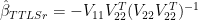

Figure 2. Diagram of TTLS Eigenmatrix Decomposition. Dimension of matrices is (n,1)= (n, q+1-r) * (q+1-r,1) * (1,1).
Total Least Squares is a special case of Truncated Total Least Squares in which regpar=q. In that case, the coefficients only involve the (q+1)th eigenvector (which has the smallest eigenvalue) and the TLS coefficients can be expressed as:
(6)
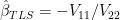
The coefficients for Truncated TLS with regpar=1 are proportional to rows 1:q of the eigenvector corresponding to the PC1. The coefficients for TTLS (regpar=2,…, q-1) are, in a sense, intermediate between the PC1 solution and the TLS solution, yielding a one-parameter arc of line segments, analogous in a sense to the one-parameter arc between PLS and OLS solutions that we’ve observed in previous posts e.g. here – a picture that I personally find very helpful in de-mystifying these things.
Averages from USV^T Expansions
An extremely important property of the above algebra is that TTLSr (TTLS using regpar=r) yields a matrix of coefficients 
Because the TTLSr relationship can be reduced to a matrix of coefficients
The demonstration below uses the “associative” property of matrix multiplication. First we denote the TTLSr estimate as follows:
(7) 
where 

The original PC decomposition of the AVHRR data (denoted below as 
(8)

where 

(9) 
where 

The Antarctic average (denoted here as 
(10)

where 
(11)
In other words,
(12)

where 

(13)

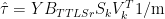
Thus,
(14)

using the definitions above for the V matrices.
This can easily be changed into a function of pc and regpar. I plotted the contribution

Figure 3. Effective weights in Antarctic average of 30 stations with: prior infilling of stations with more than 240 values; regpar=3, pc=3, coefficients from calibration period.
The 1957-2006 trend of this particular reconstruction is 0.061, noticeably less than the Steig trend using regpar=3, pc=3 and similar to values obtained through other methods. I’m not sure why this yields a lower trend than the RegEM’ed method. I’ve got a couple of variations in the method here : (1) the calibration coefficients from the calibration period were not “updated” from information from the reconstruction period. The interpretation of such updating is discussed in Brown and Sundberg 1989 (and isn’t easy); (2) the station data is infilled first, prior to calibration to the PC data and “short” stations weren’t used. Perhaps these lead to a difference.
IMO, it’s extremely important to keep in mind that any of these methods merely yields weights for the stations. This particular calibration ends up with relative low weights for the Peninsula stations, slightly negative weights for the Southern Ocean islands – the usefulness of which has never been clear – and relatively consistent weights for continental stations.
This sort of graph would be a helpful template for understanding what happens with varying regpar and PC. In order to end up with Steig’s trend (nearly double the trend shown here), the weights of high-trend stations have to be increased.
Trends
There’s one more potential simplification that’s useful to keep in mind. The trend of the Antarctic average can be obtained by left multiplying by a structured matrix 

(15)


84 Comments
I haven’t doublechecked the script below, but it should be close to turnkey
There can be an overfitting problem, though not serious as in the inverse case. But with Brown’s CI formula the uncertainty in is taken into account, which helps to cope with this kind of overfitting. MBH98 calibration residuals -method neglects the uncertainty in
  .
.
MBH applies this procedure, but the very next step is variance matching of the reconstructed U-vectors, which brings it back to somewhere in the land of continuum regression.
Question to the statisticians on board:
Is there a “Gauss-Markov theorem” for TLS ?
So this is a case of Principal Component Regression, where the “ordinary” variance based PC selection rules should be used with extreme caution.
Take a look at these studies which address the methodology and it’s weaknesses.
Christiansen et al (2009)
Click to access reconstr_reprint.pdf
The underestimation of the amplitude of the low frequency variability demonstrated for all of the seven methods discourage the use of reconstructions to estimate the rareness of the recent warming. That this underestimation is found for all the reconstruction methods is rather depressing and strongly suggests that this point should be investigated further before any real improvements in the reconstruction methods can be made.
Von Storch et al (2009)
The methods are Composite plus Scaling, the inverse regression method of Mann et al. (Nature 392:779–787, 1998) and a direct principal-components regression method. … All three methods underestimate the simulated variations of the Northern Hemisphere temperature, but the Composite plus Scaling method clearly displays a better performance and is robust against the different noise models and network size.
Riedwyl et al (2008)
This paper presents a comparison of principal component (PC) regression and regularized expectation maximization (RegEM) to reconstruct European summer and winter surface air temperature over the past millennium. … For the specific predictor network given in this paper, both techniques underestimate the target temperature variations to an increasing extent as more noise is added to the signal, albeit RegEM less than with PC regression.
I believe they are addressing the issues that you raise.
Re: Vernon (#4),
None of these papers goes back to the linear algebra. They all deal with things empirically. None of these papers considers, for example, the connection between PLS coefficients and OLS coefficients ir the “space” of coefficients.
IMO my post on the von Storch pseudoproxies a couple of years ago does a better job of explaining the phenomenon. http://www.climateaudit.org/?p=707
Steve, if I follow your linear algebra, it appears as if A-hat retains no original values from the AVHRR decomposition. It looks to be the linear combination of the predictors (ground) only. That is equivalent to what I dubbed the “model frame” in my reconstructions.
.
In Steig, he tacks the solution onto the end of the original values from the AVHRR decomposition, which creates a discontinuity at t=1982. This discontinuity (as well as the fact that there is a higher trend in the AVHRR data than the ground data) is what causes his higher trends. The higher trends in Steig are a combination of insufficient resolution with PCs, discontinuity where the solution is spliced to the actual data, and a higher trend in the AVHRR data itself (which, in turn, is at least partially due to discontinuities between the satellites).
.
If so, that is why your trends match other methods. If I have a chance today, I’d like to email you my “methods” notes I’m making on the differences between Steig’s method and mine.
Re: Ryan O (#6), here will be different from the unspliced estimate
  , which I think that I kept track of in my RegEM-TTLS routine. The “model frames” will be a little different. I’m not sure exactly how much impact the “updating” of the coefficients through the EM process actually has – as compared to the splicing.
I didn’t much like the term “model frame”; I, for one, didn’t understand exactly what it was, so I presume that others didn’t either. The
Re: Steve McIntyre (#10), I’m not sure I understand where the original PCs are retained, as it looks like U-hat = Y B-TTLS only includes information from the stations and the TTLS coefficients. A-hat is calculated using U-hat and the truncated AVHRR eigenvalue and eigenvector, none of which contain the original PCs.
.
In the R version of the TTLS routine (if I am interpreting it correctly), the solution is only recorded for missing values:
.
where kmisr represents the row numbers for the missing values, which are estimated from the TTLS coefficients (B)and the available values (kavlr). The original values aren’t “spliced” precisely; instead, the solution is not recorded for them. This is not the same as U-hat, except where values are missing.
.
As far as “model frame” – it was a poor descriptor. Been a while since I did any real math. Haha. A better descriptor would be “solution”.
Re: Ryan O (#17),
Ryan, I’m not trying at this point to represent all the aspects of their quirky methods in one bite. I’m trying to see how close I can get to their method using methods that are known to the civilized world.
I’m not resplicing in this algebra. I’m doing it like a statistician would – estimate coefficients and then compare the fitted values to the actuals. Obviously I wrote my version of the algorithm anticipating this sort of analysis by keeping track of the fitted values as well as the respliced matrix. (I sort of like the word “respliced” in this context – sounds like re-fried: the Mexican food algorithm.)
The EM algorithm does two things though – let’s say we have a B matrix of coefficients from the calibration period and add more information from the reconstruction period station histories. The EM method (even without resplicing) “updates” the coefficient estimates and I think that I extract these coefficient estimates in my version of the algorithm (which we can probably simplfy a little as we go along). It will be interesting to see how much difference the “updated” coefficient estimates have.
Brown and Subdberg 1989 seem to suggest that the additional information is best used to decide whether the calibration conditions have varied with new information, and, in the sorts of problems they have in mind, whether this mandates a new calibration. They don;t specifically consider reconstruction-type problems where there is no possibility of recalibration, so their remarks are not exactly geared to the issue that concerns us, though they are geared to a related issue and are the closest contact with civilization that I’ve seen for these methods, though the connection is not obvious or easy to make.
Re: Steve McIntyre (#20), Cool . . . thanks for the reply. The reason for the question was to make sure I understand the source of the lower trend you calculated. The weighting method you use seems mathematically identical to retaining the full solution. If so, that means my erroneously dubbed “model frame” reconstruction – henceforth called the “full solution reconstruction” – is identical.
.
And yes, your version does extract the updates to the coefficients.
Re: Ryan O (#6),
I don’t think Dr. Steig figured out that your information is surface station trends weighted by covariance as their paper was intended to be.
Re: jeff Id (#11), Yeah. They misinterpreted what their method was doing. Their method only does that in the pre-1982 timeframe, and then they splice the satellite data on the end of that. Their description of what they do in their paper is misleading. I don’t think it’s intentional; I think they really didn’t totally understand what it was they were doing.
Re: Ryan O (#19),
I’m not sure it was a misinterpretation, Dr. Steig’s latest answer to the one question I got through was revealing in that he recognized the potential need for satellite recalibration – which was my intent in asking in the first place.
I think it may have been an over-zealous interpretation (without crossing the polite boundary). When writing as a group, not everyone is as confident as everyone else.
Kenneth about lost his mind when he figured out what was happening in the comment thread on tAV.
Re: jeff Id (#22), Yah, you’re right. He does explicitly mention that.
Re: Ryan O (#6),
The “discontinuity where the solution is spliced to the actual data” seemed intuitively to me to be a poor practice when Ryan O and Jeff Id explained to me what I thought was being done.
Although I do not follow exactly all the linear algebra, these discussions do help me obtain a better grasp of what the methods are capable of resolving. I look forward to reading Ryan O’s forthcoming exposition and Steig comparandum and more threads intros like Steve M has produced here.
Scott Brim, I hope you and others who might potentially feel unworthy will join me in continuing to read and attempting to understand what has been made available to us by way of a few blogs.
Re: Ryan O (#6),
I’m sure that you’re right empirically about the splice being the main factor in the trend.
IMO the real benefit of the approach outlined above – and not everyone probably appreciates it – is the decision to view the RegEM as an “updating” of a calibration process a la Brown and Sundberg 1989 (whioh is online in the CA pdf directory.) Brown and Sundberg 1989 is not easy going. I’ve been working on it off and on for a long time.
Re: Steve McIntyre (#16), I need to read that one. I imagine it will be painful, however, but if I ever hope to have any competency in interpreting this stuff, I need to get a better handle on the theoretical side of things.
Warmers of my acquaintance strongly question the value and credibility of everything that has been done so far by CA, WUWT, the two Jeffs, RyanO, Lucia etc. concerning Steig’s paper — the primary objection being that none of the people participating in this exercise have any recognized climate science credentials.
If one were to examine the various facets of knowledge and experience that one would expect to be necessary in examining Steig’s Antarctic paper, what percentage of the total background of the required knowledge and experience would each of the following areas cover?
— Climate physics and dynamics
— Sensor physics and dynamics
— Data collection/management methods and techniques
— Statistical analysis methods and techniques
— Integration of physics/dynamics, data, and statistics
If those doing a critical examination of Steig’s paper don’t include recognized professionals in each of these areas, does the examination have any real credibility?
Re: Scott Brim (#7), Of course credibility is irrelevant. If the methodologies are valid it doesn’t matter who does it. It also doesn’t matter if it’s posted in a “peer-reviewed journal”, or other ivory tower. Arguably something will get more peer-review here than anywhere else.
Re: Jeff Alberts (#8)
Re: Kenneth Fritsch (#9)
Re: Steve McIntyre (#14)
Re: Craig Loehle (#15)
.
Comments/responses to Scott Brim (#7) continue in Unthreaded-n+2. I’ll copy the original over to unthreaded so that everybody knows what the topic is.
Re: Scott Brim (#7),
Scott, what are your credentials for making these observations? Surely, I, as a layperson, can read the evidence and analyses, and with some effort on my part, make a reasonable judgment of the validity and uncertainties in the arguments.
Is there some secret handshake required to join those “who can understand”?
Re: Scott Brim (#7),
Scott, my response would be that the calculations carried out by Steig et al are statistical. The authors of Steig et al are not statistical authorities. The articles have clearly not been reviewed by statistical authorities, but have been weakly reviewed by other climate scientists, no better qualified than the authors in statistical matters.
Re: Scott Brim (#7), The questions that need to be addressed at this point are: is what was done valid, statistically robust, numerically stable, etc. These are mathematical, statistical, and data analysis questions. No one here is addressing the meaning of the outcome (such as relation of the 3 PCs to air circulation patterns), because if the methods are unstable or invalid why would you try to “explain” them? While Mann thinks of himself as an expert in this area, there is quite a bit of complexity (and many pitfalls) that requires untangling and that some of the posters, notably Steve, the 2 Jeffs and Ryan, have done an amazing job of.
Now THAT is a tutorial.
BTW, tex typo: /hat\tau should be \hat\tau
“…though they are geared to a related issue and are the closest contact with civilization that I’ve seen for these methods…”: Let’s face it, when this guy wants to write, he can write.
Steve,
Cool post BTW. I’ve set it up to make plots at a variety of regpar = pc = whatever. It’s not that unsimilar to Steig et al result although not exactly the same.
There are a couple of lines that don’t work right in the script but it doesn’t take much to get it going.
At PC=3 the whole continent is pretty well featureless with slight warm spot in the peninsula. At 7 the peninsula shows strong warming with the north pole and left side of Ross ice shelf showing cooling.
I don’t think it’s that much different than the solution Ryan gets with RyanEM.
Re: Jeff Id (#27),
To be more clear, the trend distribution has the same features as we expect from PCA – same as Steig paper. The overall trend is much lower because it’s SST data. So in the end the features plot similarly to RyanEM.
snip – please don’t editorialize on this sort of thread.
There’s that link again, well I spent a couple hours playing with this method and put up a few graphs. I’ve got to figure out how to stop the link backs.
Forgive my simple mind.
It occurred to me that a simple test of infilling methods would be to take complete time series of data, remove data corresponding to other incomplete data series (or other random selection) and then run infilling and compare to the original.
Because there are 3 manned Australian bases on the coast of Antarctica (Mawson, Casey, Davis), I’m making a collection of annual data with some metadata for each of these from various sources. Just about finished Casey. Seems to me that when you are chasing small differences in late-stage statistical dissections, you need to know the variability of the figures at the ground stations.
I have Casey almost ready to report on Excel (sorry, yes, Excel). Here are a couple of condensed lines to show what the larger picture has. Ryan at 19 mentions year 1982. It was an anomalous year on the ground also, the coldest reported below for many years. Numbers below are degrees C, annual average from monthly or daily data, primary source BOMTmean, which is already homogenised to an unknown extent. I have done a tiny amount of guesswork infill. There are weeks at a time when the daily BOM data do not look the same as surrounding periods (such as in no places after the decimal).
Year,GISShomog,Giss Raw,KNMI,BOMTmean,BOMcd
1981, -7.26, -7.37, -7.31, -7.32, -7.34,
1982, -10.33, -10.48, -10.22, -10.25, -10.28,
1983, -9.03, -9.10, -8.98, -9.07, -9.12,
There was also a station change of some 3-4 km, betwen 1969 and 1990, but it is hard to determine how long the old data continues in the dataset. There was a change in reporting period from daily to half hourly in August 1999 and to one minute in May 2002, but again info is short on the transition method and instrument changes.
I think I am correct to state that the BOM declined to use early data from 1956 to 1969, but it appears in GISS and KNMI, quality unknown.
Is anyone interested in the full exercise? Where is the best host to place it as I do not have a website.
Re: Geoff Sherrington (#32),
Geoff, e-mail me; dhughes4 at mac dot com
thanks
One other thing that deserves mention about Steig’s use of RegEM.
.
Steig does a single RegEM step. He puts and incomplete PCs alongside the incomplete ground records and imputes the whole thing together.
.
To me, this does not make sense. The PCs are not temperatures; they are essentially coefficients for a map. What physical reason is there to allow this abstract quantity – which does not represent a temperature at a point – to affect the estimation of the ground temperatures? TTLS assumes errors in both Y and x and minimizes the combined error. However, when you impute everything together, an error in Y does not mean the same thing as an error in x even though they are scaled to unit variance. Y is a temperature. x is a coefficient that is later interpreted by the eigenvector. RegEM, however, can’t tell the difference – it assumes they are the same thing.
.
Additionally, the PCs are satellite derived, and in several posts across the blogosphere, multiple people have discovered properties of the AVHRR data prevent it from being a drop-in replacement for ground temperatures. In practice, imputing everything together this way leads to obvious artifacting even at low regpars (just look at the Antarctic tiles). This means that some type of calibration needs to be performed between the two. Steig’s method of mushing everything together at once violates the integrity of a calibration because it allows information from outside the 1982-2006 calibration period to affect the fit during the calibration period.
.
To address these issues, the reconstructions I did use a different method than Steig. Rather than mash everything together at once, I first impute the ground stations without the PCs. This eliminates the concern about the difference in meaning between ground station errors and PC errors, because the PCs are simply excluded.
.
I then take the fully populated ground matrix, place the PCs next to it, and run RegEM again. Because the ground stations are fully populated, the integrity of the calibration is better preserved. The estimation of reconstruction period values can no longer affect calibration period values because all of the calibration period values are fixed.
.
The last difference is that I use the full solution for the PCs – i.e., the best fit between the PCs and the ground stations – in place of any original values. Otherwise, you have the situation where the post-1982 portion is entirely satellite derived and the pre-1982 portion is entirely ground station derived, which presents a visually obvious artifact at the splice.
.
This (combined with his assumption that # of PCs and the regpar setting must be held the same) is why Steig gets worse validation statistics as he increases the number of retained PCs. His method allows all kinds of strange artifacting – as the tiles show.
.
If, however, you separate the ground station imputation and the calibration steps, the artifacting largely disappears.
.
A related question, Steve, is if Mann does a similar thing to Steig in his reconstructions. If Mann mashes everything together and does it all at once, that might explain the “64 flavors” that B&C noted. The mashing-method solution is much more unstable than the separated imputation/calibration solution.
Re: Ryan O (#34),
Ryan – a couple of points. Try looking at Brown and Sundberg 1989 see the CA/pdf/statistics directory. You may not be able to follow it but there will be phrases here and there that are helpful.
MBH98 did not use RegEM and it used a different calibration method than TTLS regpar=3.
You can logically separate the two things – which would be an interesting experiment.
We could add a module replacing the TTLS step with GLS/”Classical” calibration, but still do the updating. I think that the GLS/”Classical” which MBH inadvertently did would be like a very low order regpar. Probably about the same as regpar =1.
Seeing the interaction of PC and regpar also gives a new light on an aspect of MBH that’s never been discussed and which is highly relevant to Steig – how MBH retained temperature PCs. There have been endless discussions about tree ring PCs, but temperature PCs are a different ball of wax. Take a look at the MBH98 text on this in light of Steig. MBH98 uses 1 temperature PC in their early reconstruction and uses more with more proxies. The reasoning on this selection is almost nonexistent/nonsensical, with the outcome more or less arriving from outer space, but after arrival, becomes adopted as a precept, cargo cult, as it were.
Re: Steve McIntyre (#35), I really like the idea of replacing the TTLS step with a GLS calibration, if only to see what the differences are. It would seem that you would be able to use the GLS calibration as an “idiot check” on TTLS.
.
<–rereading MBH.
.
My eyes rolled into the back of my head the first time through B&S. That one will require some effort.
Re: Ryan O (#34),
This is an extremely important point and one which is completely ignored by the authors of Steig et al. Although the satellite PCs could be viewed as temperature “averages” because they are linear combinations of satellite grid measurements, the RegEM procedure as implemented gives each station record (heavily imputed or not) a weight equal to that of each PC since the TTLS step is done on the correlation matrix. I don’t see any parameters in RegEM to allow for changing that – did I miss something?
IMHO, this approach is substantial improvement, but it does have the drawback of not allowing the satellite data to contribute information for the infilling of the station data during the time period when both are present (which might be a desirable capability). A possible alternative might also be to try a three step procedure:
Step 1: Infill the stations using the satellite data for the 1982 to present (possibly only from the grid values in the immediate vicinity of the stations. However, I thought that in his apologia pro opus sua on RC, Dr. Steig seemed to imply that there was not much of a match due to some sort of “geographic considerations”.
Step 2: Use only the station results from the previous step to extend the infill only to the stations in the period prior to the satellites.
Step 3: Use the completed station data to extend the satellite results (PCs or otherwise) to the earlier era.
The rationale for this would be that the satellites can help infill the stations when both are available. Since they were not available in ther earlier period, after step 1, they would have little extra information to offer in step 2. The procedure could conceivably be more stable with fewer moving parts at any given stage.
Re: RomanM (#37),
You didn’t miss anything. There are no parameters for that.
.
I tried this, and in the end, I agree with Steig’s comment. The satellite temperatures are not drop-in replacements for ground temperatures. There are discontinuities between the satellites, and, in the case of NOAA-11, there is a large discontinuity that occurs at 1993. Other users of AVHRR data have noted and documented this in the literature.
.
This results in the residuals between ground station temperatures and satellite temperatures having a strong dependence on time, with that dependence split into well-defined groups corresponding to coverage of a particular satellite. When you use the satellite data as you suggest, the artificial trends in the satellite information (due to the discontinuities) get directly transferred to the ground stations. This was originally the purpose of my calibration step that Steig disliked. Try to take care of the discontinuities before substituting satellite data for ground data. (The step later evolved into a diagnostic to see which reconstruction method best prevented the artificial trends from being communicated to the ground stations. It is presently meaningless except as a diagnostic.)
.
However, I think there is an additional wrinkle we can give this to make it work. I haven’t had time yet to try. But here’s what I was thinking:
.
With the exception of NOAA-11, within a given satellite period, the residuals don’t show this dependence. So what if we:
.
1. Split the ground stations and satellite data into periods by satellite.
.
2. Place the ground station data (with some minimum completeness requirement) next to the raw satellite data for each of these periods and impute (or some other form of regression since there will be a 1-to-1 correspondence between a particular satellite grid and a particular ground station). In essence, this allows us to find a different calibration constant for each satellite based on the observed offset between the satellite data and ground data. This will only infill stations that have overlap with that particular satellite. We repeat this for each individual satellite.
.
3. Collate the imputed ground station data (some of which will still be incomplete, as there are periods for certain stations that have no data for a particular satellite) and then, with this more complete matrix, infill back to 1957.
.
4. Use this completed station data to extend the satellite results.
.
One of the unquantified uncertainties in the Steig method (and in my alteration of the method) are spurious correlations. Doing it as you suggest – with the additional step of restricting each infill to a given satellite period – would seem to greatly reduce the chance of spurious correlations as RegEM will be better constrained by having more 1982-2006 data to guide the imputation.
.
Steve: In B&S, what mathematical operation do their primes indicate – like (X* – mean.X*)’ ? The reason I ask is that the denominator of their diagnostic for determining when recalibration is necessary looks curiously close to the denominator for CE.
Re: Ryan O (#38), I should mention that the lack of match between satellite and ground, IMO, has nothing to do with Steig’s explanation of “geographical considerations”, and has everything to do with uncertainties in cloud masking and offsets between the satellites.
Re: Ryan O (#38),
Ryan, I have notes on Brown and Sundberg 1987 here http://www.climateaudit.org/?p=3364.
I haven’t worked through 1989 in the same detail – it’s on my to do list. ‘ is usually a transpose in his notation. It looks like * are centered.
Re: Steve McIntyre (#40), Excellent. Thank you!
Re: Steve McIntyre (#40), I think I need to read 1987 and maybe 1982 to understand 1989. The 1989 paper assumes much prior knowledge, none of which I have. Best to start at the beginning!
Re: Ryan O (#42),
I think this might be a good starting point.
Re: Jean S (#43), Thanks!
.
Ah, my reading list grows . . .
Re: RomanM (#37),
I’m not sure it matters, using Steig’s method, that the satellite PCs are weighted the same as the surface stations despite not being temperature measurements as such. The average temperature trend that comes out of applying RegEM is virtually unaffected by what weighting is applied to each of the satellite PCs (providing of course that the inverse weighting is applied to the reconstructed satellite PCs output by RegEM). RegEM (of at least the TTLS variety, with regpar=3) does indeed appear to give each observation series equal weight, but independent of any weightings applied to the series. However, the number of satellite PC series included does affect the result. Using the first three PCs but including them twice in RegEM, giving 48 data series including the 42 surface stations, increases the 1957-2006 continent-wide average temperature trend from the RegEM reconstruction by 0.020, from 0.119 to 0.139 degreeC/decade (and changes the 1957-1981 trend from 0.258 to 0.289). In case RegEM was affected by having duplicated columns in its input matrix, I also tried making the second set of three PCs equal to the first set with random N(0,1) noise added. The result was unaffected. Including the set of three satellite PCs three times increased the trend further, with a somewhat smaller rise of 0.015, to 0.154 (1957-1981 trend 0.313). Conversely, duplicating the 42 surface station series in the RegEM input matrix (which effectively halves the weighting of the satellite PCs) reduces the 1957-2006 average temperature trend by 0.013, to 0.106 (1957-1981 trend 0.239). Including four copies of each surface station series further reduces the average trend by 0.005, to 0.101 (1957-1981 trend 0.230). Extrapolating on a diminishing returns basis, this suggests that if the satellite PCs had no influence on the surface stations reconstruction (as per Ryan O’s separate imputation method), the Steigian 1957-2006 average temperature trend would be slightly under 0.10 degreeC/decade.
I have extended the approach outlined above to go some way towards the three step procedure outlined. I used multiple copies of both the surface station and the satellite PC series, but in all except one of the copies of the satellite PCs I filled 1957-1981 with random N(0,0.1) data so that they could not, by being imputed, influence the imputation of the surface stations. The resulting 1957-2006 average temperature trend was 0.105 degreeC/decade when two sets of data were so used, and 0.100 with four sets.
Re: Nic L (#46),
The TLS procedure as implemented in RegEM gives all the all the variables (predictors and predictees) equal status by default becuase all of the variables are scaled to equal variance before the SVD decompostion is carried out. The orthogonal distances which are being mninimized in PTTLS(from the data points to the subspace) are equally affected by PCs and stations alike.
From a theoretical viewpoint, this does not make a lot of sense since it reduces the entire data set to the equivalent of three stations and then apparently uses those “PC-stations” to reconstruct the entire continent. Your duplication of the three PCs will certainly give more importance to the PCs, but what I was thinking of was scaling the PCs individually higher (possibly proportionally to the eigenvalues – I’d have to think about that). Because TLS is not scaling invariant (from some R experimentation, duplicating a variable is not equivalent to multiplying it by 2) this would be somewhat different from what you did.
It would not be that difficult to implement in the regem.m program by altering the scaling step (and scaling back part after TTLS). It might also have implications for calculating the uncertainties, but I don’t think we have been using that part.
The more reading I have done on this, the more I wonder why they are doing it this way…
Re: RomanM (#49) and Re: Nic L (#46), I ran reconstructions where I imputed each PC individually. I put each PC next to a fully imputed ground station matrix and ran RegEM. After I was done with each one of them, I collated them to do a reconstruction.
.
The answer is almost identical to putting all the PCs in there at the same time and imputing, at least at regpars less than 10. Due to no overlap in the 1982-2006 timeframe (as you are imputing them individually), they do get increasingly correlated at the higher regpars and some fairly obvious overfitting begins to occur. But at regpars up to about 9, the answers are nearly identical.
.
So if the same answer comes out whether the PCs are imputed together or they are imputed separately, then it would seem that at least the relative scaling between the PCs is not that critical. The scaling between ground stations and PCs is a different story, though.
.
However, with a little point-of-view change, I think that problem disappears, too. 🙂 I think some of our difficulties in trying to figure out the best way to do this results from being fixed to the general concept behind the Steig reconstruction. But I think that Steig approached the problem from the wrong angle.
.
For a while I’d been doing the reconstructions by using basically Steve’s A-hat with no original values retained. I felt this was conceptually more valid, but until Steve did the linear algebra, I couldn’t really explain why. Now I feel more confident that I can explain why splicing (or retaining) the original PC values causes all kinds of problems. So here goes . . .
.
As Roman mentioned earlier, Steig’s process is an extrapolation. He retains the 1982-2006 portion of the PCs. In order to be able to combine the post-1982 portion with the imputed portion legitimately, they have to mean the same thing. This leads us to consider all kinds of ways to mess with RegEM – weighting, duplicating, etc. – to try to preserve this meaning during the imputation.
.
But instead of approaching this as an extrapolation, let’s think about it as an interpolation.
.
The EOFs have two components: a spatial map and a PC. The PC is merely a time series of coefficients that describe how important the associated map is at each point in time. The map simply converts the coefficient into a “partial” temperature anomaly at each grid location.
.
Assuming the AVHRR data is a reasonable approximation of surface temperatures, the stations that show correlation with a particular PC during calibration will necessarily be located at grid cells with a high weight for that particular EOF. RegEM will minimize the total square error, which will (1) be more dependent on the stations than the PC, and (2) be more dependent on stations that show correlation. Because those stations are located in grid cells with high weight, this means that the PCs will take on values that best explain variance at the station location. If you are attempting to use the PCs to predict temperatures BETWEEN stations – and you take the station temperatures as “truth” – then this is exactly the behavior you want. TLS will converge to a solution that best replicates the temperatures AT station locations, and the covariance information in the remainder of the EOF map fills in the areas between stations.
.
In the interpolation case, you want to minimize the contribution of the PCs to the solution. You want the ground stations to determine the solution. The purpose of the PC is to use the covariance information in the spatial map to fill in the blank areas based on station temperature. The purpose isn’t to try to drive the imputation. So you want RegEM to minimize station error, not PC error. In this case, if we did want to try to scale the PCs, we know exactly how we’d want to do it: scale them as small as possible.
.
In my opinion, the best way to approach this is not to try to figure out how to make an extrapolation valid. The best way is to simply use it as an interpolation because the tool used (RegEM) naturally lends itself to the latter case.
.
Thinking about it this way also helps make it clear why the Steig method is conceptually not valid (well, helps me, anyway). Because of the way RegEM computes the solution, the pre-1982 stuff is essentially an interpolation with the stations as the anchor. The post-1982 stuff is 100% satellite. The two periods are not measuring temperatures in the same way.
.
Anyway, that’s the approach I took for my reconstructions. Instead of trying to figure out how to properly extrapolate the satellite PCs, I decided instead to use station data as anchor points and the covariance information in the PCs to interpolate the remainder of the grid. This requires that the post-1982 PCs be replaced by the TTLS solution. Retaining the original satellite derived values is not conceptually valid.
Re: Ryan O (#51),
Ryan
I agree with you that it makes sense to replace the post 1982 PCs with the TTLS solution (=the model frame). As well as the reasons you give, I think that doing so should reduce the effect of drift, bias and discontinuities in the satellite measurements, without having to make ad hoc corrections.
If you have modified Steve’s regem_pttls script to output the solution for all points, not just missing ones, could you possibly post or upload the modifications, to save me and others time?
In the meantime, I have used my weighted RegEM version to impute what I think is a close estimate of the 1982-2006 solution for the satellite PCs. With sum of weightings =10 for the PCs used for imputing the surface stations in 1982-2006, the 1957-2006 average trend falls from 0.0405 (per my previous post, using the actual satellite PCs post 1981) to just 0.0146 C/decade.
Re: Nic L (#53),
I haven’t modified the pttls script for that. Instead, I modified Steve’s regem_pca. I call it “regem_ipca” in the script. It outputs both the spliced solution and unspliced solution:
http://noconsensus.files.wordpress.com/2009/05/recon.doc
I would recommend letting the whole script run the first time through, as it will demonstrate what the different commands mean.
As far as the satellite PCs go, I long ago gave up on them representing actual surface trends no matter what you do. Here’s an excerpt from a draft Jeff and I have been batting around to explain. If I have additional time later, I can provide links for the references. Fig. 1 is not complete yet, so I don’t have anything to show from that, but the text should give you the general idea.
Re: Ryan O (#54),
Ryan O, I believe your comment here answers a question that I posed at AirVent on comparing the trends for 1982-2006 for AVHRR and surface station data.
After reading all these analyses, I see a conundrum developing whereby the effort has revealed so many separate weaknesses/errors in the Steig et al. (2009) paper that when it comes time to put that case forward, either in the blogdom or in a peer-reviewed paper, it becomes difficult for the reviewer of that work to comprehend and fully appreciate all of the evidence and in some cases remembering all these separate points. On the other hand, if one issue at a time is put forward, such as Steig chose to cover in his RC reply/tutorial on over fitting, it would appear that it becomes easier for the defenders to arm wave down a single issue and reference peer reviewed papers that do not always apply directly to the case at hand.
I think that MM have had that experience in publishing and the blogdom in their critiques of Mann’s reconstructions and its progeny. I do not have an immediate answer for this apparent problem, but I think it is one well worth contemplating.
Re: RomanM (#49),
I think that duplicating a PC series in RegEM is in fact equivalent to scaling its effective weight by sqrt(2). Having now looked in more detail at Steve M’s RegEM PTTLS script I think that each data series can very easily be separately weighted by making the following changes to it:
Replace
regem_pttls=function(X,maxiter=30,tol=.01,regpar=3,method=”default”,startmethod=”zero”) {
with
regem_pttls=function(X,maxiter=30,tol=.005,regpar=3,method=”default”,startmethod=”zero”,weights=1) {
and
D=sqrt(diag(C))
with
if(length(weights)==1) { D=sqrt(diag(C)) } else { D=sqrt(diag(C))/weights }
weights, if specified, is a vector with the same length as the number of columns in X, with each element being 1 except for data series that are to be scaled up or down. For example, in the Steigian case, setting the last three elements of weights to sqrt(3) gives a 1957-2006 continent-wide average temperature trend of 0.154 C/decade, the same as when the three satellite PCs are triplicated.
I have experimented with weighting the three satellite PCs by their standard deviations (=square roots of the eigenvalues), scaled to give more or less total influence on the imputation than i the base case. Doing so with sum of the weights of respectively 1, 3 and 10 gives 1957-2006 trends of 0.0993, 0.1274 and 0.2236.
With sum of weights squared =3, which I think gives the same overall influence of satellite PCs as in the base unweighted Steigian case, the trend is 0.1220. This is only slightly higher than the base case of 0.119.
These results support Ryan O’s conclusion (in #51) that the relative scaling between the PCs is not that critical, but that the scaling between ground stations and PCs is a different story.
In principle, giving a relatively high aggregate weighting to the satellite PCs post 1981 does not seem unreasonable, as they convey information from the whole of the continent. However, I think we all agree that in the pre 1982 period it is illogical to allow the imputed satellite PCs to influence thesurface station imputation (which in turn influences the imputed satellite PCs).
Further to my earlier post (#46) about using multiple copies of both the surface station and the satellite PC series, with all except one of the copies of the satellite PCs filled with random data, I have improved this approach by using just two copies of the PCs, the first being minimally weighted in proportion to the PC standard deviations (sum of weights = 0.1) with NAs in 1957-1981, the second being higher weighted, in the same proportions, in 1982-2006 with N(0,0.1) data in 1957-1981. With the sum of the second weightings =1, the 1957-2006 trend was 0.0957, but this fell dramatically to 0.0405 C/decade with sum of weightings =10 (some 3.68x higher weighted than in Steig’s base case, in terms of sum of squares). Changing the first set of weightings to equal weighted (each 0.1) had virtually no effect on either of these results.
I was able to back calculate station weights from Steg et al and determine the linear weighting value for each temperature station. Four peninsula stations were flipped into anti-temperature mode and about 70% of the reconstruction trend came from the peninsula.
The post is at the pingback link #47 above.
This isn’t exactly a TTLS question, but since it’s related to the Steig recon, figured this was as good a place as any. The question comes mainly out of thinking about commentary by Jonathan Baxter and Carrick at tAV.
.
I’m having a hard time wrapping my head around how the climate field reconstruction techniques are physically valid. The main problem I have with them are negative coefficients – be it predictor weights in a TLS calculation or negative values in the EOF eigenvector. No matter how I try to justify this, I cannot think of a way around these two problems:
.
1. The temperature mean at each predictor location needs to be stationary – yet these techniques are used to describe a situation where the mean, at least, is not stationary.
.
2. While I understand how principal component regression can be valid, I cannot see how this is expanded to include the validity of using the eigenvector to extrapolate the entire field (as opposed to extrapolating the specific location of the predictor and leaving locations without a predictor undetermined).
.
Negative Weights/Coefficients
.
Negative weights imply divergent or oscillatory behavior. In the case of predictor weights, it is not physically possible for this type of inverse relationship to be valid throughout all ranges of temperature. In other words, falling temperature for predictor A cannot always imply rising reconstruction temperature because atmospheric mixing places a maximum limit on temperature gradients. This limit for each location insofar as reconstructions are concerned is not explicitly calculated, nor has such a calculation been shown to be possible with the precision needed for climatology.
.
So if negative weights do not represent divergent behavior, they could represent oscillatory behavior. This interpretation has a distinct problem during extrapolation as well, since correct prediction requires a stationary mean for both the predictor and the predictands. However, reconstructions such as MBH and Steig show nonstationary means for the predictors.
.
I do not see how it is valid to extrapolate using negatively weighted predictors (given that both the predictors and predictands are measuring the same quantity; in this case, temperature). Negatively weighted predictors with nonstationary means seem almost guaranteed to produce unphysical results. To me, it seems that the signs of the predictors should be a diagnostic for the reconstruction: strongly negative signs indicate that the reconstruction is likely to be invalid.
.
EOF Eigenvectors
.
While I have no problem with principal component regression in concept, the idea of performing a principal component regression in order to predict PC loadings and then reconstructing the field using the eigenvector also seems physically unsupportable.
.
The first reason is similar to the above observations – most of the higher-order PCs have areas of strongly negative coefficients. A nonstationary mean for the predictors translates into a nonstationary mean for the loadings, which translates into unphysical behavior with respect to the areas of negative coefficients.
.
The second reason is that the PC decomposition of a data set does not yield factors that are directly interpretable as physical effects. I have yet to find a publication using a synthetic data set that demonstrates PCA properly uncovering the known factors. Even on the simplest sets – such as the ones used in the North 1982 publication – the orthogonality and maximum explained variance constraints force mixing of modes. More complex ones like some of Jackson’s sets or the ones in ICA papers show such complete mixing that the known factors are completely unintelligible in the eigenvectors. And all of these sets are FAR less complex than climatological data sets. Nor can rotations be shown to resolve this issue, especially with factors that just happen to have approximately the same response to the predictors during the calibration period (such as CO2 and temperature).
.
If the EOFs do not represent isolated factors – but rather a combination of factors – then the regression will yield invalid results unless either the relative importance of each mixed factor does not change significantly with time or that the mixed factors all have approximately the same response to the predictor such that distinguishing the factors is unimportant. I have yet to see a paper that shows that either one of these conditions is even likely to be met. In the case of the paleo stuff, the latter option is definitely not even close to being met, and the former is highly unlikely to be met. Instead, I see papers where the EOFs are directly interpreted as having physical meaning, and then this is used to justify the extrapolation. Or, alternatively, no physical interpretation is done and EOFs or predictors that do not display the desired correlation are simply discarded.
.
For the moment, the whole idea of CFR boils down to using empirically determined correlations to extrapolate data with complete disregard for causality and easily calculable diagnostics that the reconstruction is likely to be invalid.
.
I’m hoping that RomanM, Steve, Jean, UC, Hu, or someone else with a better handle on CFR can comment. 🙂
Ryan, I also would like to hear their comments. I think Roman touched on this when he was discussing a different result using PC’s than the raw data and he couldn’t see that it was the same thing. I don’t want to put words in his mouth.
One detail above I think I can comment on is the negative coefficients on high order pc’s. The orientation of the higher order EOF’s is a difference between two groups of data. If the data is autocorrelated spatially I imagine the data as Steve showed it. Since the higher PC’s are representing basically an oscillatory difference between these groups of data, the sign of the EOF is 100% arbitrary and negative coefficients are justifiable.
In the case of the Antarctic, we have basically quadrants oscillating back and forth in PC2 and 3, so the physical explanation would have to relate to weather patterns in those areas. I don’t understand how the reconstruction is supposed to work when the PC’s are trendless oscillations between half-continents. It leaves my head fuzzy.
Re: Jeff Id (#58), Yep . . . which is, to my understanding, what Carrick and Baxter were trying to say. They were simply conflating the station weights with the covariance information in the eigenvectors. I’m not sure either of us ever convinced them of that, though.
.
The part that bothers me is this (oversimplified for understanding):
.
Let’s say you have an eigenvector with half of the continent at a +1 coefficient in each cell and half at a -1 coefficient. When the PC loading is 0.5, then this particular EOF will predict a +0.5 anomaly in half and a -0.5 anomaly in the other half. Let’s assume that this pattern is a result of seasonal oscillation.
.
Now let’s assume that you have one predictor available. It happens to be a station located in the +1 region. When you regress the PC against the station, you will obtain a relationship between the PC loading and the station. You then proceed to extrapolate temperatures by extending the PC back in time using the predictor.
.
What happens to the reconstruction if the actual continental mean in 1957 is one degree less than it is in 1982?
.
Instead of showing the same oscillatory pattern centered 1 degree lower than in 1982, the reconstruction will show the oscillatory pattern to have the same mean with a larger (2 degree peak-to-peak) amplitude.
Re: Ryan O (#60),
I agree with your comment. With enough PC’s I believe it should revert to the natural state but what does it mean for a few. Steve made a comment about using a high number of PC’s with low regpar. This makes a lot of sense to me because you retain your cov, but I keep getting sidetracked and haven’t finished. Why not do all the pc’s at regpar=5 or 3 one at a time?
Too many pc’s won’t cause overfitting and the data is basically temp info so why not? The theory is that high pc’s are noise, but that is for signal extraction purposes, we’re extracting covariance.
Re: Jeff Id (#61), Actually, I’d done that a long time ago and never bothered to post it because I couldn’t figure out in my head why it would be a better method. It felt like a better method, but I couldn’t explain why. Here’s the results with a 13-PC solution:
.
.
.
.
.
.
.
.
.
Note how stable the solutions are. Past regpar=3 it really doesn’t matter until you hit regpar=10 and then you start getting overfitting. By regpar=15, the overfitting is massive.
.
If you retain, say, 20 PCs instead, the solution is still pretty much the same:
.
.
.
.
Anyway, if you impute the PCs separately, I can’t see any reason for high regpars. The question is, how do you know ahead of time (before you actually do the reconstruction) that regpar=3 is sufficient? That was one of the questions I couldn’t figure out. Otherwise, you can always be accused of simply selecting the reconstruction you like best.
Re: Ryan O (#62),
Just to clarify what I said before. I have no idea what the best Regpar is for TTLS. I beleive it is responsible for the overfitting and my thought is now that the standard PC selection methods relate to the creation of a trend rather than the replication of continental temperature information.
So the point I’m making is – There is nothing which can be considered noise in the PC’s. There is a point where it doesn’t matter any more because the signal doesn’t affect the result, but including more PC’s doesn’t cause overfitting.
The reason to do it one at a time is simply to make sure they are independant during EM. You explained to me before it made little difference with 3 ish pc’s (from memory) but I wonder what difference there is at 20. This guarantees separation of the imputed signal.
I think I’ll drop a question over at statpad to see if Roman will take a look at your original comment.
Re: jeff Id (#64), While I didn’t find the final answer to be much different, the answer requires a much lower regpar when you impute them separately. You need regpar=6+ when you impute them all together, but only regpar=3 when you do it separately.
.
The drawbacks to separately are that it takes more time and that it is more susceptible to overfitting if you use higher regpars because you don’t have the 1982-2006 overlap for the PCs to keep them from becoming too correlated. (On the other hand, the overlap period itself is problematic when you impute them together because you end up with random sign flipping at higher regpars . . . so the regpar thing is probably a wash.)
.
The big benefit is exactly as you say: preventing the PCs from interacting during RegEM. With the scaling step, I think you eliminate my last concern with it, which is deciding ex ante what regpar should be.
Re: Ryan O (#66),
If I understand then we’re proposing a RegEM on all station data first followed by individual regem’s on as many PC’s as is required to define the answer one at a time all with low regpar, using the Xmis matrix for a RyanEM 😉 surface station data reconstruction.
I’m guessing the answer changes very little after 15 or 20 pc’s anyway.
By doing the process this way, we eliminate the problems with choice of regpar and PC number. I’ve got another post on the hockey stick almost finished, after that I’ll get back to this.
————-
Reposted.
Ryan, I also would like to hear their comments. I think Roman touched on this when he was discussing a different result using PC’s than the raw data and he couldn’t see that it was the same thing. I don’t want to put words in his mouth.
One detail above I think I can comment on is the negative coefficients on high order pc’s. The orientation of the higher order EOF’s is a difference between two groups of data. If the data is autocorrelated spatially I imagine the data as Steve showed it in the antarctic chiladni pattern. Since the higher PC’s are representing basically an oscillatory difference between these groups of data, the sign of the EOF is 100% arbitrary and negative coefficients are justifiable.
In the case of the Antarctic, we have basically quadrants oscillating back and forth in PC2 and 3, so the physical explanation would have to relate to weather patterns in those areas. I don’t understand how the reconstruction is supposed to work when the PC’s are trendless oscillations between half-continents. It leaves my head fuzzy.
I hope steveM takes the time to look at this result.
I think your method for RegPar choice in your post on tav is as good as any other. What I’m wondering about is a RegEm of surface data only as in your post, followed by an individual RegEM of each PC through the whole set. I can’t think of a good reason not to include every single pc. Either way, if you have it done, a short post on that couldn’t hurt.
Look at how stable the result is. – How many PC’s should you retain, — enough so that it doesn’t make a difference in the answer.
The graphs look like the surface data. The ideal reconstruction might be RyanEM with all pc’s yet low regpar.
Nice stuff.
Re: jeff Id (#63), Actually, I had another idea that might be able to get us to regpar=1. What if I take the correlation matrix and multiply the surface stations by the appropriate eigenvector coefficients for the PC I am imputing? That will guarantee that the stations in high weight areas of the eigenvector are selected as PC 1 during RegEM. I suspect the reason that the higher regpars are needed is to ensure that you capture enough modes such that at least one of the PCs is located in a high weight area.
.
The other improvement might be to remove surface stations with less than a certain number of points – say 100 or so – to avoid spurious correlations during the RegEM of the surface stations.
The trouble that I have with deciding on the “right” PC or regpar is that the decision is not connected back to a statistical model. The connection is not easy – I’ve been working on it off and on for a long time and haven’t got the connection that I want. The alternative at present is merely showing that results are not robust to these parameters.
There are several key issues in the methodology here: 1) the use of PCs; 2) the use of truncated TLLS in inverse calibration; 3) infilling.
My own instinct is that serious problems begin with the shift from “classical” calibration Y ~X to “inverse” calibration X~Y, because the inverse calibration introduces “regularization” problems that don’t exist in classical calibration. (I think that this is separable from the use of an expectation-maximization algorithm for infilling, such as the one used in my alternative algorithm, but I’m not 100% sure).
It’s also my guess that negative coefficients get introduced with inverse calibration.
If one uses regpar=1, it seems to me for the reasons indicated in the post that you get a calculation that is homeomorphic in some sense to classical calibration even though it’s framed in inverse regression terms (and not a felicitous way of expressing things.)
My recommendation at this point is to step back a little from the Antarctic calculations and to review the Smith and Reynolds methods and the Beckers-Rixen method. (We got a nice post here from one of the Beckers-Rixen authors and this is worth following up.)
Smith and Reynolds use a lot of PCs and it would be interesting to understand their reasoning and methods a lot better both for the Antarctic study. Plus the SST data is interesting in its own right,
I realize that people are screeching for a study on Antarctica, but their interests tend to be topical rather than in the method per se.
Re: Steve McIntyre (#68),
.
I think you will like this result, then:
.
.
Or maybe you want to use 50 PCs instead:
.
.
The interesting thing is that, in comparing the 13 PC to the 50 PC reconstruction, you can see some Peninsula information is contained in the higher-order PCs. The rest of the continent seems to be well-resolved at 13 PCs.
.
This would seem to support the suspicion I had that the need for higher regpars in RegEM was to capture enough modes to ensure that at least one of them was located in a high-weight area for a particular EOF. This is why regpar=1 just smeared the whole continent out when the ground stations weren’t weighted by the eigenvectors. But by scaling the ground stations based on their respective eigenvector weights, you don’t need to capture the higher-order modes.
.
Regpar=1, baby! 🙂
.
I’m going to write up a post for this over the next couple of days for tAV.
Can’t be right? – looks too much like the instrumental record to me? 🙂
Oh, one other note . . . the script (which I will post on tAV after I clean it up) also allows you to perform the reconstruction either:
.
1. As an extrapolation of the satellite PCs
.
2. As an interpolation between ground stations using the satellite-determined covariance
.
The script to use the eigenvector weights requires a scaling factor. Setting it high results in the ground stations being selected as PC 1 in the truncated SVD imputation; setting it low results in the PC itself being selected in the truncated SVD imputation. This speaks to RomanM’s comment in (#37) about being able to change weights.
.
Basically, I multiply the eigenvector values for the station locations through the ground station matrix prior to doing the SVD in RegEM. That emphasizes the importance of stations in the high-weight areas, so it makes the region where the EOF explains the most variance drive the imputation. The scaling factor then determines how much of PC 1 in the truncated SVD RegEM is the satellite PC or the ground stations.
.
For the plots above, I used a scaling factor of 1, which weights the ground stations and PC evenly. If I set the scaling factor lower, the reconstruction becomes an extrapolation. With a scaling factor of 0.25, the 1982-2006 unspliced solution is nearly identical to the raw satellite PCs. The 1957-1982 period looks quite different, but the overall trend is only about 0.03 Deg C/Decade higher.
.
I intend to use this functionality to show that there are indeed offsets between the satellites. It’s pretty simple – you simply withhold a particular satellite, run the reconstruction, and subtract the 1982-2006 portion from the raw satellite PCs. The offset shows up in the difference. 🙂
.
With this modification, we can compare the results of satellite extrapolation vs. a ground station interpolation. The latter was what Steig et al. stated was their intention, so it is the most applicable reconstruction. However, it’s probably worthwhile to analyze the former to attempt to see what the differences are and attempt to determine why they might be different.
Nice job Ryan, It’s always a surprise when things work how you expect.
I need the script to understand the scale factor fully so I’ll look forward to your post.
My own sense of what is a “right” way of approaching this problem is based on some personal experience with the vagaries of estimating ore reserves from drill core – a problem which has a long history (giving rise to “kriging” and “nugget effect” – and one where you often get to compare your estimate against an actual.
Like Antarctica, you can have small high grade ore zones (a peninsula) if you will and low grade zones.
The idea of presenting investors or securities commissions with ore reserves in which you’ve used PCs or regpars makes my head sore. There have been lots of interesting and colorful incidents in mining history, but ore reserves calculated Mann-Steig style would cause hilarity. (Standard methods are area averaging with an area of influence assigned to each drill hole.)
To the extent that one is trying to calculate a “right” history, I’ve seen no evidence that one can do better than area averaging,
One further consideration that is worth tying into this.
I think that the concept of spatial autocorrelation is pretty fundamental to the exercise. On that basis, PCs simply generate Chladni patterns and the entire Steig premise of physical meaning to these things evaporates.
If you have spatial autocorrelation, I think that one should be able to show that area weighting has relatively attractive statistical properties. There might be something in the kriging literature on this – I confess that I’m not as familiar with this literature as I’d like to be. While I’m familiar with ore reserve calculations, it’s not something that I did professionally.
Re: Steve McIntyre (#73), While there are many similarities to an ore reserve calculation, I think there are some important differences that may drive a different method.
.
In ore reserve calculations, there is not a time-varying factor. Where the ore is today is the same as where it was yesterday. That means the covariance between high quality deposits and low quality deposits is constant in time.
.
In the case of Antarctica, the covariance is not constant in time. This would seem to require a regression method rather than kriging, though I’m not sure you could state at the outset that a regression method would inherently be more accurate. But you can say at the beginning that by doing kriging rather than regression that you are by definition giving up the possibility that you can track changes in covariance.
.
Also in Antarctica, you have a period with 100% coverage of the grid (satellites) and a period with spotty coverage (ground stations only). This means a decision needs to be made on which sources are to be used; and, if both sources are to be used, the best way of combining them. Personally, I like the idea of using the satellite covariance information to do the interpolation.
.
AFA Chladni patterns go . . . I’m not sure I see a problem with it in principle, as long as you include enough modes to accurately recover the initial information. It’s like modes in wavelet analysis. Individually, they’re often meaningless, but that does not mean that they cannot be used in a meaningful fashion.
Kriging, would create a pretty picture with a resulting total trend similar to closest station area weighting. I don’t think there’s much we can do better than area weighting. However, if the area can be determined reasonably by RegEM and the data is localized as it should be, that would be pretty good too and would take into account the climatology a bit more. The resulting trend should be similar to area weighting but I don’t know what the real improvement is, it looks cool though.
In Ryan’s plots above there is a large section of the east side of Antarctica with no data at all and in its place warming data is there. I doubt very much that this section is real trend and none of these methods can bring it out because you can’t create data that doesn’t exist. Still I think Ryan’s regpar=1 high pc version eliminates the choices we were struggling with as far as how to choose these values in non-arbitrary fashions.
Claims of standard PC selection methods are unrelated to reality. Even the more sophisticated ones are highly limited in their application range and just give someone a spot to throw a reasonable dart. That’s why I find Ryan’s result exciting, as many PC’s as are required to resolve the detail and regpar=1. If there was enough surface data, it might give an accurate (near area weighted) trend.
BTW, I went back to the Beckers-Rixen post. The first time it went up, there were almost no comments and it was hard to understand. Now its a two minute read, thanks for that. Ryan has been using that method in his work.
Re: jeff Id (#74), Yah, no matter how we slice this, there will be areas that all we can say is, “I don’t know”.
.
At the moment, my biggest “I don’t know” is why the Community can’t seem to bring themselves to admit this.
Having done this kind of thing myself thirty years ago for a evaluation of the future economic potential of a disseminated gold deposit, and now after having followed this blog for about three years, I can say with some confidence that the climate science equivalent of “kriging” has to be “kluging”.
.
Continuing the last post:
My own past experience in gold, silver, and uranium tends to confirm this opinion. Not to say that my 1979 copy of Geostatistical Ore Reserve Estimation didn’t cause my brain cells to overheat back in its day.
RomanM: In the case where I weight the stations by the eigenvector coefficients and impute each PC separately, it seems like I should take the imputed PC, multiply the left eigenvector through, and subtract that from the stations prior to moving on to the next step.
.
The reason is that during the SVD, PC 1 explains a certain amount of the variance. Then PC 2 explains a certain amount of the remaining variance . . . and so on. Subsequent PCs are based on the remaining information, not the original information.
.
So it seems that the appropriate way to do this is to impute each PC based on the remaining station variance – not the raw data.
.
Thoughts?
Re: Ryan O (#79),
Ryan, it’s not clear to me that, under the circumstances, any “correction” is necessary.
I assume that what you are talking about here is as follows:
— The station data is infilled for the entire period first (either by itself or by using the satellite PCS to infill the post 1982 period and then extended to the earlier times).
— This infilled station data is used to extend the PCs.
If this is the case, then the station data is being used merely to predict the PCs and predicting the first PC does not “use up” information which is no longer available to predict the others. In a simple regression situation, if I am predicting two variables using a fixed set of predictors, the least squares solution for the simultaneous prediction is numerically the same as that of the separate individual regressions. Of course, this latter fact is not true for total least squares regression, but the underlying concepts appear to be the same.
Where your notion of adjusting the predictors comes from is the decomposition of the variability of the station data in which quite correctly, if a PC summarizes some of the variability of the station temperature structure, it should be removed from the data before the next PC is calculated. That is not quite the situation you are looking at.
You could also try the following sequential approach as a sort of in-between approach: Take the station data and impute the first PC, Then attach that to the station data matrix and use the new structure to impute the second PC (keeping the firsr PC imputuation fixed), etc. This way, previous PCs have an effect on the later imputations (but not vice versa).
If I missed a step on what you are doing, please correct me and I will comment further.
Good stuff on getting a better handle on a not-so-transparent technique.
Re: RomanM (#80), I don’t know whether this will change your opinion, but I think I need to get off my ass and write down the math for the latest algorithm. The algorithm no longer does a simple regression of station data and the PCs; it explicitly uses the eigenvector to weight the station data and performs the regression on the weighted matrix. The steps to get to this point are: ) for the AVHRR data:


 next to the completely imputed station data.
 and rescale such that the range of
  equals 1. This is for consistency – it maintains the same scaling of station data relative to PC regardless of which PC you are imputing.
 by a weighting factor
  (default to 1). The reason for this is to provide a means for performing the reconstruction as an extrapolation of the PCs (small
  ) by de-emphasizing the station data, or as an interpolation (large
  ) by emphasizing the station data. How this works is clear from the next step.
 , series where the PC explains the most variation will be selected as the low-order PCs, while series where the PC explains little variation will be relegated to the higher-order PCs. This ensures that the stations representing high-weight regions are represented in the SVD of the matrix. It also maximizes the contribution to the total error of the high-weight stations during the OLS regression, which causes the high-weight stations to drive the imputation.
 is apparent: small
  weights errors in the PC high, so minimizing imputation error in the PC minimizes the overall error. This results in an extrapolation of the PCs. High
  weights errors in the stations high, so minimizing imputation error in the stations minimizes the overall error. The latter forces the PC to the station solution. This results in anchoring the original eigenvector
  at the station values during the reconstruction, and using the coefficients to predict temperature at locations where the stations are not present – in other words,
  becomes analogous to the kriging estimator for kriging.
 .
.

 step. If you did not do this step, then I agree that removing the contribution is unnecessary. However, weighting the stations changes the regression results. As each PC has its own set of station weights in
  – and these station weights were derived by explaining remaining variation after the prior PCs had been calculated – then for each subsequent regression to be valid, you need to remove the contribution of the prior PCs. Failure to do so results in convergence to a different (albeit similar) answer.
.
1. Perform RegEM on the station data without the PCs.
.
2. Find the PCs (
.
.
3. Extract the spatial weights for each PC at the station locations. Let’s call this matrix
.
4. Place PC 1
.
The next few steps take place within my modified RegEM algorithm:
.
5. Scale all series to unit variance.
.
6. Scale the station data by the appropriate vector from
.
.
7. Multiply
.
8. In RegEM, we now have the following matrix:
.
.
We perform the SVD directly on this matrix. Because each series is scaled by the appropriate constant from
.
Now the purpose of
.
9. Once the algorithm converges, we extract the imputed PC,
.
10. At this point, we can recover the temperature contribution from the imputed PC 1:
.
.
The reason I felt it was necessary to remove the contribution from PC 1 before calculating PC 2 is because of the
.
When I do this by removing the contribution of prior PCs, the net effect is to give a reconstruction solution that takes higher regpars to achieve if the contribution is not removed. I’m not totally sure I’m on the right track, though.
.
Re: Steve McIntyre (#81), This latest algorithm does explicitly use the geographic information. Also, it’s faster than the previous ones – so I’ve done test reconstructions using 100+ PCs. We could easily do reconstructions using ALL of the PCs, which makes determining the truncation point simple. After ~13 it doesn’t matter. You don’t have to worry about including too many – because you can’t include too many.
.
Also, while I am interested in the average, I am also interested in the geographic distribution of the trends since it was the odd geographical distribution that made the Steig paper so noteworthy. The last 7 methods (or thereabouts) Jeff Id and I have done all show the same geographic distribution. The only outlier is Steig’s.
.
*presses submit and prays the Latex worked…*
Re: Ryan O (#82),
 ) next to the completely imputed station data.
 )
)
.
Eqn. in #2 should read:
.
#4 should read: Place PC 1 (
.
Eqn. in #8 should read: (
.
Those “PCscaled” and “eigenscaled” notes should be part of the subscripts. They’re just descriptors.
Re: Ryan O (#83),
.
Stupid human.
.
Eqn. 8:
Re: Ryan O (#84), I give up. Eqn. 8 describes a matrix with the scaled station data times placed beside PC 1.
Re: RomanM (#80), You are indeed correct . . . and after I figured it out, I feel a bit stupid.
.
I had thought that such a correction improved the verification statistics. However, I mis-named the variable that I applied the correction to, so all of my test reconstructions were run with just the stations scaled by the eigenvector weights and no correction. When I figured that out and actually applied the correction, the verification statistics were degraded a bit.
.
And then, after thinking about it, I started wondering why I thought that would work in the first place.
.
Sometimes . . . not so smart is I.
One point about infilling using E/M methods (or PCs or this sort of thing) – they don’t explicitly use geographic information.
On the other hand, area-averaging methods such as ore reserves explicitly use the geometry.
Here are a couple of thoughts.
I think that we can say that there is very strong evidence for spatial autocorrelation with more or less negative exponential decorrelation. (Far more evidence for this than Steig’s 3 physical modes). This should enable some analytic simplifications that simply cut through the PC problem altogether. I don’t think that there’s any evidence of real modes. And I don’t see any purpose in truncating things merely for computational reasons without trying to think through the math. Maybe there’s an analytical sum of series somewhere.
Second, our interest at any given time is not really in the infilled values at particular stations but in the Antarctic continental average at any given time given spotty measurements. On a spatial autocorrelation basis, this is an inverse of the Fourier heat equation (which also makes sense from first principles) – which is going to be approximated by the disk case where you have a value at the center and some values on the boundary. My guess is that the analytic solution to this sort of problem is a form of area-averaging. These things usually end up with a geometric connection.
Okay . . . I’ll have to learn Latex better. Here’s the equations using Word. Some of the symbols are a tad different due to Word’s limitations:
.
Ignore all of the above crap. Working with Latex apparently drained my brain.
.
I redid this explanation in Word and posed it as a question to Dr. Beckers. The .pdf – with a MUCH improved explanation of what I did – is here:
.
Click to access Dr_Beckers.pdf
5 Trackbacks
[…] by Jeff Id on June 3, 2009 Steve McIntyre developed a method Link HERE to reconstruct historic temperatures using truncated total least squares calibration. This method is […]
[…] the heart of where the trends in Steig et al. came from. Steve M did a post on TTLS reconstruction TTLS in a Steig Context which makes the point that despite the PCA and truncation the result of RegEM is still a linear […]
[…] the heart of where the trends in Steig et al. came from. Steve M did a post on TTLS reconstruction TTLS in a Steig Context which makes the point that despite the PCA and truncation the result of RegEM is still a linear […]
[…] said in his post on TTLS – Truncated total least squares. Because the TTLS relationship can be reduced to a matrix […]
[…] eigenvector matrix V is used in the TTLS calculation. See previous CA discussion here. Let’s suppose that there are p proxies and one instrumental series in the network. V will […]