In examining the Briffa Yamal chronology, there has been a lot of emphasis (IMHO, correctly) placed on both the cherry-picking and the low core counts of the proxies which extend into recent times. However, the chronology also depends on the various methods used to adjust for various known biological effects and on the choices for how various parameters are estimated. Although this has been pointed out by various blog commentators (see, e.g. Jeff Id, comment 67 from Re-Visiting the “Yamal Substitution” and his posts at the Air Vent), few attempts have been made to examine the resulting effects in a quantitative fashion.
In order to understand what follows, it is necessary to place the chronology construction on a more solid mathematical footing. Statisticians prefer to create a model: Identify the variables and the relationships for the measurements in the physical situation. Within the model, the appropriate analysis becomes more apparent and meaningful with regard to the underlying physical situation.
The Model
In the case of the Briffa tree ring widths, it is basically assumed there are three basic elements which affect a tree ring on a given tree. First, there is the natural growth pattern, Growth(Age), that the tree undergoes as it ages. This is assumed to depend solely on the age of the tree and (when using RCS) to be the same for all trees in the regional sample. It should be noted that Age is itself a function of Year and Tree so that it is not really a “new” variable in the model. Secondly, there is the effect of the climate, Climate(Year), during the given year in which the ring formed. Finally, there are those factors which affect only that tree, Error(Tree, Year), such as soil, moisture, and the environment surrounding the specific tree in question.
Next, we need to specify how these factors fit together mathematically. There are two simple forms that could be used:
Additive: Ring Width(Tree, Year) = Climate(Year) + Growth(Age) + Error(Tree, Year)
and
Multiplicative: Ring Width(Tree, Year) = Climate(Year) * Growth(Age) *Error(Tree, Year)
The additive model is not particularly realistic for tree rings since the ring width can never be negative which means that the distribution of the “Error” term will be limited from below by the current Age and Climate. There is no real symmetry possible for the distribution and the variability will generally not be the same across all Year and tree combinations. Since the latter is usually a requirement for the proper application of some commonly used statistical procedures, the analysis becomes problematical.
The multiplicative model is better from a variety of viewpoints. Effects of the factors have a simple interpretation. A change of a fixed amount in a factor produces a corresponding percentage change in the tree ring size rather than a fixed +/- amount. When the tree is young and ring widths are larger, an increase in temperature of several degrees would likely produce a proportionally larger increase in ring size than when the same tree is considerably older so this model can be more realistic.
There is another benefit to this model. A simple log transformation converts it into an additive model:
log(Ring Width(Tree, Year)) =log( Climate(Year)) + log(Growth(Age) )+ log(Error(Tree, Year))
with the corresponding benefit of all of the statistical machinery that is available to analyze linear models. At the end, the factor estimates can be exponentially converted back to their original form.
Within these models, the tree ring chronology is nothing more than an estimate not of a “signal”, but of the sequence of parameters: {Climate(Year)}.
The details of the Briffa RCS fit are as follows:
Growth(Age) = A + B e-C * Age
where A, B and C are coefficients which are to be estimated from the existing data. In Steve’s RCS emulation of the Briffa calculation, this is done by using a non-linear least squares fit to all of the available ring data.
In my opinion, this method (not Steve’s emulation of it) has several severe drawbacks. The first is that this methodology assumes that the “error” terms are additive – not multiplicative. Since least squares does not like to see very large deviations from the growth curve, the choice of the coefficients is dominated by early age rings where the variation is likely to be the highest. Secondly, the sheer numbers of early age rings (each tree has to go through age one to get to age two, etc.) exacerbate the effect further. Thus the RCS fit will be dominated by the early years of each tree. If all the trees had similar growth patterns, it might be less of a problem, but that would need to be checked as part of any analysis.
Now, once the growth curve has been estimated, the next step is to adjust the tree rings for age. In the RCS methodology:
Adjusted(Tree, Year) = Ring Width(Tree, Year) / Growth(Age)
This tells me that to make any reasonable statistical sense, the dendrochronologist must be using a multiplicative model. If you divide the additive model, the Climate effect and the Error effect on a tree becomes contaminated by the Growth effect and will now be different for trees of unequal Age in a given year. Note also that the variability of the adjusted value will depend on the age of the tree since the Growth is itself an estimated effect.
Next, in estimating the climate effect, we average the values:
Adjusted(Tree, Year) = Climate(Year) *Error(Tree, Year)
over all Trees in that Year to get the chronology of Climate estimates. This tacitly assumes that the Error terms average out to 1 (by itself not a restriction) and that dividing by the estimated Growth curve does not produce bias of varying amounts which could be a serious consideration depending on the distribution of Ages for a particular Year. However, the variances of the terms being averaged arenot the same because of the adjustment step and this means that any confidence intervals for the estimate may vary from year to year depending on the ages of the trees contributing to the that year’s average. Because of these and other considerations, calculating the climate estimates in this fashion seems to be poor statistical procedure.
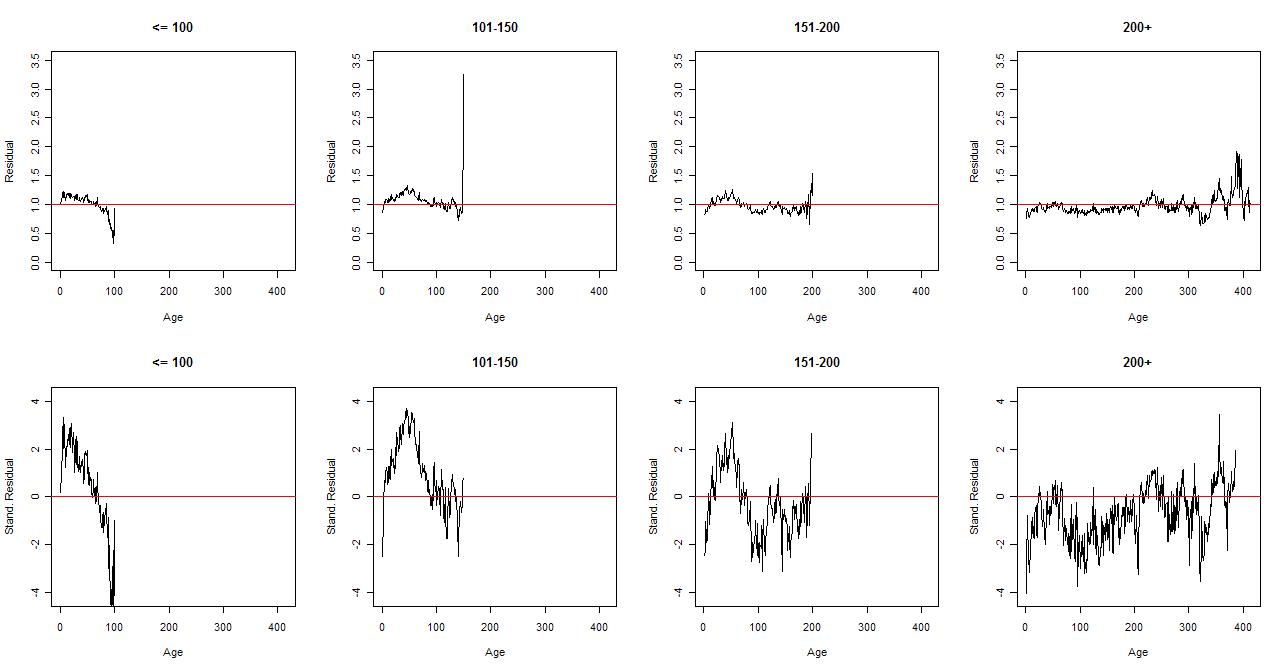
Finally, dividing the Adjusted values by the estimated climate gives the residuals, i.e. the estimates of the Error terms. An examination of the residuals is a good way to check whether the model is appropriate. There should not be any relationship between Age and residual or with any other variable. However, with 40892 residuals to look at, this is not simple. What we will look at is how the residuals are distributed by the length of the record (“lifetime”) of the trees.
The Residuals
The initial data is the matrix yamal generated by Steve’s R script in comment 1 of the thread, Yamal – A Divergence Problem. From the same script, the function RCS.chronology will be used to calculate the adjusted values and the chronology. From these, the residuals for all of the ring widths can then be calculated.
The data was divided into four “life” groups: less than 100, 101 – 150, 151-200, and greater than 200 years resulting in frequencies of 54, 76, 58 and 64, respectively. Since there are still too many residuals for the separate plots to be informative, the averages for each age year were calculated. As well, since different numbers of trees contribute at different ages, both the raw averages and the standardized averages (by subtracting the number one and then dividing by the standard error) were calculated. The results for four “life” groups were plotted separately:

There seem to be some pretty clear age-related patterns in the mean residuals plots that may result, possibly, as a result of the inadequacy of the particular growth curve as applied in the RCS process.
Ring Widths
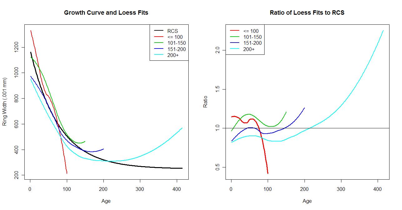
In order to look at it a bit further, we can look at the estimated growth curve and compare it to the actual distribution of the ring widths themselves. Again, because of the enormous number of rings involved, we will use a lowess fit (with default R span parameter) to the ring widths using the age as the predictor. The fit will have a similar smoothness to the negative exponential used by Briffa.

In the ratio plot, the patterns seen in residual plot are evident. What was not seen quite so strongly is the way that the negative exponential growth curve severely underestimates the ring widths of the long lived group.
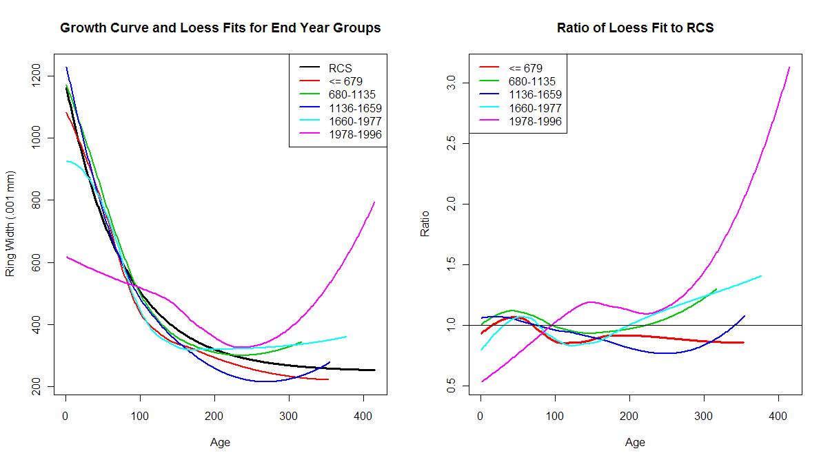
For a final analysis, the trees were regrouped by the end year of the tree’s life. The year ranges were Before 679, 680-1135, 1136-1659, 1660-1977 and 1978-1996. This allowed the mixture of trees with a variety of lifetimes and could examine whether there were changes in the tree behaviours over time. A similar lowess fit was used as in the above graphs:

I was somewhat surprised how reasonably closely the growth curve fit most of the historical group distributions. Well, except for one group …


503 Comments
I had a slight computer problem which killed my R script for this. I will reconstruct it tomorrow morning and post it along with the relevant data. Sorry about that. 😦
Re: romanm (#1),
The shape of the segregated tree series in the head post should be of no surprise given the shape of the Yamal RCS chronology. The climate signal is dominant in the last trees of the series and so the difference from an RCS fit should be the greatest for this group. You’ll only get all your curves to overlay if there is no climate signal.
Re: Layman Lurker (#51),
Delayed Oscillator makes some very pertinent points. Using least splines seems the way to go here. I tried to use Steve’s R utilities for this, but I don’t seem to get a valid chronology by just replacement of
RCS.chronology(tree,method=”nls”)by
spline.chronology(tree,tag=”COFECHA”)
Steve McIntyre (#48), what is required to get a spline rather than exponential RCS fit to work?
Re: Tom P (#55), you have work to finish. See bender about your assignment.
Re: Tom P (#55),
Tom, how do you know that this departure is “climate signal” and not another non-climate environmental factor with red noise like character? From my understanding, RCS cannot make that distinction.
Re: Layman Lurker (#58),
RCS by itself will just say that there is a signal that cannot be ascribed to the growth pattern at the site. But as Steve McIntyre said in the previous post, the Yamal RCS chronology has a “”statistically significant” correlation to summer temperature” with an r = 0.55 and a t statistic of 4.29.
Re: Tom P (#60),
I was going to ask the same question myself, but Layman beat me to it. Your answer does not address the issue of how much of what you magically identify as “signal” and how much is possible aberrant growth due to underestimation by the growth curve used. You still don’t seem to realize that on this web site, we don’t operate on arm waving and guesses when making “definitive” statements such as you seem prone to do.
You do this again in your comment where you claim that least splines (what are least splines) are the way to go when you clearly don’t have a good understanding and certainly no personal experience with what methodology may be available. If you did, then you wouldn’t ask someone else o provide the programming for that purpose.
Re: romanm (#64),
Please read Delayed Oscillators post:
This post will help you understand that basing an RCS chronology on a fit to a subset of the data is fundamentally contrary to the what RCS is trying to achieve. You’ll also find in this post plots of the time-varying splines fit to the data, the method actually used by Briffa rather than the exponential fit you implement here.
Re: Tom P (#68),
I think “a common age-related growth trend” is a theoretical assertion. Statistically, RCS is a specific functional form for this theoretical assertion. RCS is an “identifying restriction” (an assumption from theory, or convenience, or tradition or whatever) used to infer low frequency climate variability. But suppose there is no “common age-related growth trend.” For instance, the Majumder and Radner model implies considerable path-dependence, in particular dependence on initial local resource conditions. The debate here (at least it seems to me) is whether any such “common age-related growth trend” actually exists across trees. A very interesting debate, I might add. But if it doesn’t exist, then the identifying restriction is wrong, and the recovered low frequency variability is biased.
Re: Tom P (#68),
Yes, by all means, please tell me what it is that you think I don’t understand? The reason for the growth curve adjustment? The mathematics behind it? The statistics? I’m all ears. Please, explain it to me.
I read the blog post. It consisted of a lot of armwaving and generalities, but it really did not present any substantial rargument why the spline fit is a good approach. He claims that you can’t just use the modern trees to estimating the growth curve because of the “temperature” contamination. Well, look at the left side of the spline graph. Tell me why the RCS from the entire collection says anything about the behaviour of the early years of those same modern trees. Or they also displaying a remarkable cold period in their early life? Since the trees are not of the same age, this indicates a collective behaviour which is not necessarily temperature related. So why does the spline fit apply to this set of trees which behave so differently hundreds of years ago from the rest of the sample? I’m listening.
Re: romanm (#75), Tom is great at finding something he barely understands but which he thinks supports his position. Then he points you at it with the hopes that you will explain it to him.
I’ve now read DO and commented. In general I think he could make some contributions if he gets beyond the arm waving and actually posts data and code and takes questions and provides answers. If he doesnt post code, then I’ll just stop reading and suggest that others do likewise. Also, he has said that he doesnt read this blog because of all the negative comments etc etc etc. I won’t bash him for that, I’ll just say this. In the past I’ve read RC ( and all the comments) Rabbit ( and the comments) tamino ( and the comments) in it for the gold ( and the comments) In each and every case I found that I had this remarkable ability called choice. I could choose to go moshpit on people who were flaming or I could choose to ignore them. Now, more often than not, I choose to ignore them. It’s a great time saver. I now no longer read RC, rabbit or open mind, primarly because of their comment banning procedures which are ad hoc to say the least. DO, for now, claims that he will moderate with a heavy hand, so if folks want to they should mosey over and ask questions, leave the BS at home, be polite, and see if he can back up ( with data and code and debate) what he says.
Re: romanm (#75),
Yes, most of the Yamal 12 had their early years in 17th century, the coldest period of the Little Ice Age. Your selection of this subsample shows the precise problem of constructing an RCS curve on trees whose growth is not spread across the entire period of the chronology.
Re: Layman Lurker (#76),
It’s not contrary to my statement at all – I completely agree with what Esper says here. It’s RomanM who is ignoring Esper’s caution.
You add:
Delayed Oscillator says something rather stronger than that:
Re: Tom P (#82),
So why does the full RCS chronology on DO’s page disagree with the modern trees and show it as “business as usual” while the mid 1800’s are the coldest period? By the way, I didn’t select it. Briffa did.
Re: romanm (#83),
Because to repeat what DO said:
You add:
It doesn’t. The full RCS chronology shows the late 20th century considerably elevated compared to the rest of the series.
The 1700’s also has a depressed chronology: the RCS curve for the Yamal 12 sits below the full RCS curve in DO’s plot simply because temperatures during the period of early growth of these 12 trees were below average, if not necessarily the lowest.
Re: Tom P (#87),
It has become pretty clear that the P in Tom P must stand for Parrot. Why don’t you stop the repetition and show us that you understand at least part of what you are talking about?
You are going on and on about the “least spline” fit, but I am willing to bet that you don’t know very mch about what is being done in that fit. What sort of splines are we talking about? is the fit being done to the entire set of Yamal ring widths or to something else? Are there parameters involved which are specified beforehand or is it a cut and dried operation? Is “least squares” involved in the fitting process? What is the math behind it? What are the properties and the drawbacks to this choice of curve? Why is it better than other methods for adjusting for growth? Answer these questions before going on that we don’t “understand” what this is all about.
Stop making unequivocable statements which are merely echoes of other people whom you have chosen as the the sole authority and try to bring some intellect into the discussion. Do you not understand that quite a few of the bloggers who hang out on CA are data analyst professionals with a lot more knowledge and experience than you have?
If you can’t even explain the methodology , I don’t see much point in wasting any time in reading any more of your pronouncements.
Re: RomanM (#117),
If you are still unclear about the methodology, which replaces the negative exponential fit with a time-varying spline to ratio the individual ring measurements in RCS, please read the Melvin and Briffa paper Hu kindly references above (#96). Such an approach avoids the restrictions that have been mentioned as associated with a negative exponential fit.
Re: Tom P (#118),
i.e. I don’t know what the “spline” methods are. I saw someone push a button and it just worked.
Re: Tom P (#118),
“Time-varying-response” smoothing is an attempt to get around perceived problems with the usual spline-constructed curves, not with standard “negative exponential” RCS. The splines were either too sensitive to noise at the lightly-populated old end of the age distribution or not sensitive enough to real changes in growth rate at the young end. Solution? Make them less stiff at the young end, and stiffer at the old end. Voila!
I’m not sure the topic can even be distinguished from similar issues in nonparametric regression, because as far as I can tell spline approaches are nonparametric regression fits to observed Growth(AGE). “Standard” RCS is simply a parametric fit to the same data.
Re: Morgan (#122),
I agree. But this post was criticising RCS partially on the basis of its dependence on an exponential fit for the average curve. Although certainly common, RCS is not dependent on using such a fit and other fits have been used, including spline fits of various types.
The other aspect of this post, which is to look at the RCS average curve for subsets of the data, and then express surprise when differences are found, completely misses the point of the RCS method in the first place which is to first remove the common growth-related signal from the entire series before looking at any environmental influence.
Re: Tom P (#118),
Are you really that clueless or are you just faking it to be irritating? I wasn’t asking for you to explain it to me. I already KNOW what is going on with this stuff. I wanted for you to demonstrate that you have at least an inkling of the math behind it. So far, you haven’t done so.
I spent the last hour or so porting the Fortran 90 code from the Melvin et al paper to R, but I don’t know what values of the variable ssy were used by DO in his fit. Since you obviously have been through it, maybe you can tell me what they were (seriously!).
However, I have used my own (secret 😉 ) methodology (which has nothing to do with splines) to fit a growth curve to the Briffa data. Here is what it looks like:
What do you think? Compare to DO’s graph. How do they differ(besides my adding some red dots)? Is it better than the “least splines” fit (by the way, the words least and splines do not go together). I think so, because my method will alow for a more reasonable calculation of error bounds. Will the spline fit do that? What method did I use? C’mon, don’t be a troll. Make some substantive comments. If you can’t, just ask me and I’ll explain it to you.
[Added:] There have been several correct guesses so I will add some info on the plot. The red circles are the averages of the ring widths for each age-year.
The curve is a loess curve with span paramter = . 18, which, after some experimentation, gave a reaonable approximation to the spline curve on DO’s site. The curve was fitted not to the entire set of data but to the previously calculated set of averages, again, because the spline fit was done the same way. The R version of the loess function calculates a lot of good information about the fit which the spline program is incapable of giving. Tom didn’t guess nor did he offer any opinion on the value of my work. 😦
Re: romanm (#123),
If Tom P’s BS results in more Romanm analysis (for me to ponder and learn from) I may have second thoughts about Tom P’s bandwidth. Just a little advice, Tom P, if you decide to stick around (and learn and contribute): tighten up your replies and be more specific – otherwise it does sound like BS.
Re: romanm (#123),
So you KNOW that RCS can use a number of functions to fit the average growth curve, but you chose in your post to criticise it on the basis of just one?
So you KNOW that RCS relies on using tree growth spread through the chronology to best derive the average growth curve, but you chose in your post to split up the series by time before calculating your RCS curves?
You certainly have a novel way of sharing your knowledge with your audience.
Re: Tom P (#126),
Sigh…. Tom, what do you think the word “residuals” refers to in the head post. The residuals are the ring widths AFTER the RCS adjustment has been applied. This type of analysis is standard fare for statisticians for evaluating whether the adjustment is reasonable or whether there are problems.
If the adjustment is a good one, then there should not be any strong age-related pattern in the residuals, either overall or by specific groups. Because of earlier discussion about the effects from trees with differing lifetimes, it was worth looking at from that aspect. The first graph showed that differences in such patterns were evident for thuse trees that lived longer and shorter lives than the rest.
The later graphs were a comparison of the actual distribution of ring width sizes for these groups as compared to what was predicted by the negative exponential type of growth curve along with a demonstration of the numerical effect of making that adjustment.
Now, answer some of my previous questions in romanm (#123). Did you like the graph? Pretty good, eh? (So, I’m a Canadian).
Just the result of over 40 years of teaching this stuff. However, some of us seem unable to grasp the subtlety of the concepts…
Re: RomanM (#128),
I notice you don’t dispute my point that you incorrectly associated “Briffa” RCS solely with an exponential fit.
The later graphs are plots of the Loess fit for end-year groups – an estimation of the common signal for each group, which will include both growth and environment. If the environment is different for the different groups, there should be no surprise that these fits are differrent, or their ratios to the exponential RCS vary, as I said all the way back in (#56). Do you dispute this?
Loess might be of use as an RCS estimator of the common growth signal (if that is indeed your plot in (#123), but that estimator will be valid only if tree-ring data from across the period of the chronology are contributing. Much beyond 300 years this condition is no longer met, so the fit should revert to a flat line.
An interesting sensitivity analysis of the RCS method would be a comparison of the chronologies based on an exponential, truncated loess and time-varying spline fit. My guess in the case of Yamal would be that the choice makes little difference judging by the good agreement in Steve’s exponential-based reconstruction to the CRU archived chronology.
Re: Tom P (#167),
Tommy Petard, accusing a statistician of not being a dendrochronologist, gloating that Team Methods remain undisclosed, non-transparent, inscrutible.
.
Hey, Tom, I think Gavin would like you to share that with the Audience of the Faithful.
Re: bender (#170),
Well, they only remain undisclosed to you if you can’t be bothered to actually read Briffa’s publications to see that he uses other methods than an exponential fit for RCS chronologies.
Re: Eric (skeptic) (#169),
The question is, residual against what? The only trees that can be used for the common curve are the trees containing the signal themselves. This, more than anything Steve or RomanM have published to date, is probably the most valid criticism of the Yamal dataset. It contains few earlier trees of comparable age to the modern subset to identify the common growth rather than environmental signal.
However, there are some strong arguments that a flat line at this point in growth age is the common growth signal. Firstly if you look as DO’s spline or the Loess fit in #123, (yes, I’ve noticed your confirmation of this, RomanM), it looks quite flat from 200 to 320 years where there are contributions from all periods of the chronology. It would be strange for a growth signal to rise upwards after staying flat for such a time. Secondly, there is little reason to expect biologically a late-age spurt – earlier larger, but younger trees than the modern trees don’t show such behaviour (see the grass plots of Steve McIntyre (#48)).
In fact the latter point might be worthy of further investigation. It should be possible to see whether tree size or tree age correlates better with growth (taking into account the obvious dependency between growth and size). An RCS curve based on size rather than age would enable many more earlier trees to be used in the determination of the common growth signal for the modern trees. The resulting chronology would avoid the criticism of an inability to separate growth and environment in the recent record of the modern trees.
Re: Tom P (#171),
Don’t you dare hand-wave to me. “Briffa’s methods: there out there!” I challenge you to show me the code, or the pseudocode, or even the written English instructions. I want the *specific* instructions that you imply RomanM missed. Damn fine good luck. Really.
Re: bender (#172),
You, RomanM and others and are very fond of making your accusations of “handwaving”. But it’s a pretty feeble response when used to avoid addressing the points made.
As for an example of a documented RCS method not based on an exponential fit, I refer you to the article mentioned by Hu McCulloch earlier:
Re: Tom P (#174),
It makes you wonder the purpose of the exponential fit, doesn’t it?
Re: Tom P (#167),
Didn’t you look at the graphs or my comments? All but one of the endyr groups exhibit a similar behaviour which I remarked on as “how reasonably closely the growth curve fit most of the historical group distributions.” Although each of the trees within an endyr group experienced pretty much the same temporal environment, there was a good representation of trees at various age stages during each year. Thus, the environmental effect tended to average out and no “life” group had a dominant influence in determining the shape of the growth curve.
This was the case for all EXCEPT the modern group which went past 1978. Because the group is dominated by trees in the late stages of a long life AND we simultaneously have the same environmental effects on each tree, we run into a statistical problem called confounding. It is still possible to calculate numerical estimates of each effect, but these estimates are unstable (i.e can vary wildly) and have very LARGE uncertainty bounds. Now, perhaps you can understand why Briffa’s use of such a small homogenous sample is unfortunate and why it is important to also have a variety of ages at each year throughout the entire series. It makes the chronology in recent time extremely uncertain and the “calibration” then extends the gross uncertainty to the rest of the series.
What exactly does “but that estimator will be valid only if tree-ring data from across the period of the chronology are contributing” mean? I will guess that you meant to say what I have already explained to you earlier and that is that you need trees of a variety of ages each year in order to overcome the problem of the confounding of growth pattern with environment.
Perhaps, you haven’t noticed, but this is a blog where statistics and its proper use plays a major role. This particular procedure (in bold) must have come from a Climate Science stat course in the section lebelled Ad Hoc Methods: Make-it-up-as-you-go-along. Is this your solution to the confounding problem? Close your eyes and make-believe that the group curve no longer changes after this point (but it’s OK before that point), so it must be environmental… and we just “flatten” the curve in some undefined manner? I find it difficult to imagine that you have taken a course in statistics.
Well, by all means, be my guest. You have the data and the script that I posted earlier in the thread. I’d like to see your results. With your knowledge of loess, iIt shouldn’t be much of a problem for you to make the necessary alterations to re-run my graphs. However, remember that I used a different value for the span in the head post than in the later comparison fit to the splines. Don’t be too surprised in what you see 😉 . Maybe, from experience, you can even predict where the differences will occur without all that calculation just by visualizing some of the information contained in the graphs that you have already seen.
I am puzzled, however. You indicate that loess fails after a certain point, but you imply that the spline fit is good all the way. Why is that? What properties of the methods cause this “divergence”? What I find puzzling is just how this can be when my plot in comment #123 is virtually identical to DO’s plot of the spline growth curve. How would the chronologies for the two differ?
Re: romanm (#173),
You’re confusing a simple spline fit, which is indeed very close to a loess fit, with a time-varying spline which deals with the drawbacks of the simple spline (and loess) as described by Morgan in (#122):
Re: Tom P (#176),
Tom, I have wasted enough time with your arm waving and your inability to understand both the big picture and the sublety in this discussion. You have been asked to produce concrete information with which to back up your arguments or in the very least to demonstrate that you have a glimmer of ability to appreciate the issues of the situation. So far, you have brought nothing of value to the table.
Now, we are supposed to believe in a nebulous “time-varying spline” used by Briffa in his chronology. Your reason for it and it alone as being suitable for use here is from statements in papers by authors that you deem to be the ultimate authorities on the matter.
When necessary, you make declarations on your own without any backup (e.g.including loess in the above quote as having “drawbacks”), solely on your own “vast experience” when there is no indication that you possess even a rudimentary understanding of the procedure.
Go ahead, find the spline fit used by Briffa. When you do, give us a link so that we have something to discuss. Until then, I have better things to do…
Re: romanm (#123),
You can’t remove that uptick! That’s the signal, man!
Re: bender (#127),
It’s at around 320 years old that the uptick on the curve (either Romanm’s or DO’s) starts. For the 11 trees that have survived longer than this, 7 have their last growth in the late 20th century, and above 360 years of age all the trees stop after 1970. Hence there is indeed a very large component of any signal from that period in that last portion of the curve.
Re: Tom P (#129),
lol, you are so completely clueless.
Re: Tom P (#129),
There comes a point in an argument like this when you have to advance your own substantive arguments.
Whether or not you understand the math being employed, it is ultimately just a step in a logical argument demonstrating that Briffa’s curve is or is not an accurate representation of local temperature.
You keep on making statements about steps in the process without tying them into the logical argument.
Roman is rather plainly suggesting that you lack the capacity to do so.
If he is wrong, we are already well past the time for you to show it.
Re: bender (#127),
Good eye, Bender. However, an uptick would actually decrease the “signal” since what I’ve graphed is the adjustment. I think that DO cut off the end of his graph. The longest age tree is 415 years, whereas his graph cuts off at about 390. There’s a slight difference at the lower end as well which could be due to end effects of the spline fit.
Re: romanm (#123),
Can I guess the secret? Some sort of kernel estimate of the median width conditional on age?
Re: C. Ferrall (#130),
No, more mundane than that. I used a standard statistical procedure which would not have been in general use when the dendros twigged to their relatively easy to calculate spline. This particular procedure requires more substantial computing power. I don’t think it has been used by dendros for RCS although I have seen it used by them for smoothing purposes. I’ll put an inline explanation in my comment after Tom tells me what he thinks of it and why splines are better. 😉
Re: romanm (#123),
It’s loess. romanm, email me and I’ll tell you a story.
Re: bender (#148),
I love stories! And science! That’s why I love this site!!
Re: bender (#148),
Aw, you guessed! I have added extra information about the plot in the original comment (#123).
Re: romanm (#123),
Forgive my chiming in at such a distance from your original post but I just ead your post now and, not being familiar with LOESS, went and Googled up on it. Having done that it seems very similar to my original questions earlier in the thread about using higher order polynomials or dummies and ‘letting the data speak’. It seems that this is very much the LOESS philosophy. Those some questions come to my mind (abstracting from questions about the validity of one-size fits all). For example, why smooth at all? Why not run your regression on a full set of age dummies (and year dummies)? The extraction of standard errors is easy with this and would certainly highlight the imprecision of estimates based on a few trees. How easy is it to report standard errors around your LOESS age function? I’m guessing the end result for age would look very much like what you have plotted in post #123.
On the one size fits all question, one could augment the dummy approach to allow for different tree types. For example, add a dummy for live or fossil tree and see if it is significant – interact it with age if you want a more complicated model. Inference is then based on standard tests of significance of the variable in question.
[For those who may wonder what I am speaking about, I am suggesting an OLS regression of Log(Ring Width(Tree,Year)) on a set of approximately 1800 indicator or dummy variables. That set being around 1400 dummy variables for each Year from the start of the data set to the end of the data set and a set of 400 or so dummy variables for the age of a tree from 1 to 400 (or so). Given my background, this strikes me as a fairly vanilla panel data approach and a useful first pass to describe the data.]
Re: RomanM (#117),
Thanks much for this thread as it gives me much to think about and perhaps something on which I can comment after reading it over again.
.
If it can be shown that the RCS algorithm works better for a smaller range of tree ring ages, could one consider the trade off of expanded CIs by looking at smaller sample sizes by extracting older (younger) tree rings. I think I see a definite trend in changing the shape of the Yamal RCS chronology series by using progressively older tree ring ages. I took a look at the relationship of 101 year window of standard deviation of the Yamal RCS series to the same window for mean and count and concluded that the magnitudes of the standard deviation go with the means and not with the counts – providing I did my R code and calculations properly. (See the thread: Re-Visiting the “Yamal Substitution”)
.
Thanks also for relieving some frustrations I am having about the discussions with Tom P in the post noted above. Has not the time come to ignore him until he stops arm waving and in the meantime focus on the most interesting aspects of the subject at hand?
Re: Kenneth Fritsch (#120),
That time came a long time ago.
Re: Tom P (#68),
Not even in the ballpark here Tom.
from: Esper, Cook, Krusic, Peters, and Schweingruber, “Tests of the RCS Method for Preserving Low Frequency Variability in Long Tree Ring Chronologies; Tree Ring Research; Vol. 59(2), 2003
Contrary to your statement, this sensitivity expressed by Esper et al is to be guarded against and accounted for to prevent potential “misinterpretation of climate”. All DO does is point out that the sample size in Jeff’s CRU 12 fit is not large enough to rule out intermingling of environment inot the curve.
Re: Tom P (#68), Hi Tom P. Did DO actually use Briffa’s method?
Can you point me to the place where DO posted his code and/or Briffa’s code? That would be fun to
compare. You should know from your won personal experience that even when you have someone’s
code in hand that mistakes ( hehe) are still possible. And it’s even possible for someone to take code
posted by someone ( like Mac) modify it, post graphs, have a climate expert latch onto those graphs and the person as a ‘guru’ of sorts and find out in the end that the charts dont show what they purport to show.
Posting code is even MORE important when the person doing the analysis is anonymous. When they are known
or public, guess what? they are more likely to post good code, more likely to accept criticism, and more likely
to admit their errors and fix them.
Remembered where else it was saved:
Is there a possibility of another factor – man-made pollutants such as sulfur dioxide and mercury? Both are released in large quantities when burning coal, and both are known to leach nutrients from plants and soil. Are there any good base-line studies to isolate non-climate factors on tree rings?
Re: suddzz (#3),
Frankly, I would think that any attribution of differences to a particular physical cause would appear to be pure speculation. Thatsort of conclusion would seem to require a lot of new information.
Re: Eric (skeptic) (#4),
Yes, that is one of the effects. I do think that there are several aspects of the way the mathematics of RCS is applied that tend to bias the results toward the early years of a tree’s lifetime and in at least this case produce an underestimate of the the growth in later years. The predominence of older trees late in the series is a problem for several reasons, including the lack of knowledge of the behaviour of young trees in response to the recent climate.
I also find the apparent difference in growth pattern of trees that lived less than 100 years somewhat puzzling. it may need some furher examination.
Re: romanm (#5), Trees that lived less than 100 years (and not just measured at an age less than 100 years) are likely growing in poor conditions, which is why their short life span. Perhaps crowded or maybe diseased.
If I understand correctly the RCS underestimates the ring widths for 1978-1996 trees (by a factor of 3 in the oldest trees. Then dividing the measured width by the (3x too low) RCS growth estimate makes the adjusted width 3 times too high. Is this because there are too few 400 year old trees in the 1978-1996 category? Obviously if the intent of RCS is to remove the age-related bias from tree ring measurements, then this adjustment applied to the (presumably few) number of old trees in the 1978-1996 category is producing the opposite effect. Can we conclude that the 400 year old tree(s) in that category had good growing conditions before their death?
Re: Eric (skeptic) (#4),
Model lack-of-fit at the endpoints. Model residuals are supposed to be independent (not serially correlated). It’s a model assumption always worth testing. How about a sliding-windowed DW on the residuals?
Re: bender (#13),
Part of the effect at the endpoints in the Ring Width vs. Age graph is a result of the decreasing number of trees contributing to the loess fit as you approach the right end of the Age intervals. That is one reason for including the standardized plot as well.
But you are right. Residuals should only look like random noise.
interesting post romanm.
You should send an abstract to http://www.worlddendro2010.fi (deadline has been extended to 8 Nov 09).
What implications then does the recent study out of the Univeristy of Edinburgh have where the strongest correlation to tree growth was found with cosmic rays not temperature. Kind of questions all the fundamental underlying assumptions.
Re: Alex B (#7),
In the analysis, anything which affected all of the proxies at the same time in a similar fashion would come across as “climate” rather than growth or individual variation.
Re: Ryan O (#8),
In the end year analysis, the group dividng point were initially chosen by me on the basis of creating 4 equal size groups. After looking at the result, I subdivided the last group by splitting off the trees post 1977.
Roman, for your last analysis, are those your dates for the groupings, or were those in the original paper, or . . . ?
.
The final plot is rather telling.
Stay thirsty, my friends.
Re: bender (#9),
except for one group …
Stay thirsty, my friends.
Gulp!
The log(Ring Width(Tree, Year)) =log( Climate(Year)) + log(Growth(Age) )+ log(Error(Tree, Year)) is rather stymied by the zero ring width years.
I am truly puzzled as to how one can have a zero ring width year. I presume their presence arises by matching ring patterns before and after that year and showing that there must be a missing year.
The model Growth(Age) = A + B e-C * Age is the result of prior wisdom about trees in general and seems pretty dangerous.
I doubt that it strictly necessary, one could allow the model to be decided purely on the data in the sample on a year by year basis but the sample would have to be much bigger. That is one could make the make all three terms equivalent.
Given the sample we have one would have to say that trees get a second lease of life after about 320 which is hardly likely to be the general case.
But this is biased by the relative lack of old trees amongst the fossil trees.
Also I cannot see how one can eliminate the possibilty that the survivors in harsh centuries are not the trees in favourable locations. In harsh times only the lucky trees get big enough to select themsleves as candidates for sampling. That is that the Error(Tree) and Climate (Year) are not independent.
Alex
Re: Alexander Harvey (#10),
The zero width surprised me as well. It would be understandable to possibly have missing values due to tree damage, but no growth at all? maybe someone more knowledgeable on tree biology could weigh in on this.
One way (which I have been using to deal with this problem in log transformations is to replace zero with a small value (e.g. half the size of the smallest non-zero ring) before taking logs. The order relationship is preserved and if there are not too many of these, the effect on the overall clculation will be small.
The negative exponential growth model was developed quite a while ago before statistical methodology which used enormous calculating power (such as lowess applied to 48000+ observations over 415 predictor points) became commonly available. It seems pretty restrictive in its mathematical rigidity.
Re: Alexander Harvey (#11),
This is an excellent point. As it stands, the growth is estimated and the climate effects are estimated from the residuals of the previous estimation. Ideally, one would like to estimate all effects simultaneously. However, the large number of climate parameters (one for each year) can make this a bit of a computing problem.
The alternative is to do the estimation iteratively. It makes a lot of sense to go back and readjust the tree rings for climate effect and recalculate the growth curve continuing in this fashion until the answer doesn’t change with further calculation.
I have written such an R program using a different growth curve and it seems to work. Maybe I can talk Hu and Craig into writing a dendro paper on this. 🙂
Re: romanm (#33), the negative exponential growth model is arbitrary, and you are probably right that it was driven by ease of calculation when these things mattered. Lowess is preferable, but has the problem that any climate “signal” on time scales which are long compared with the smoothing time will simply be adsorbed into the growth curve, and so cannot possibly be revealed by this approach. This is why the dendros like RCS: they claim that it can preserve such long time scale signals. However if the RCS process uses the wrong curve to fit (which it almost certainly does) then this approach will in effect invent long time scale “signal”.
For this reason I have never (at least since I finally grasped Steve’s explanation of RCS) believed that tree rings can be used to obtain climate information over time scales longer than a few decades. The approach of Moberg et al. seems the only reasonable way to incorporate dendro information.
Re: Jonathan (#35), It shouldn’t matter that the growth curve could be impacted by long term climate changes, provided the tree ages are uniformly distributed across the time axis. There could be effects where a periodic climatic effect causes die-off and makes it more likely that (e.g) a spurt at 50 years age occurs in 1800, 1850, 1900 etc – but if that were the case, it should be visible in the RCS residuals?
Re: romanm (#33),
So where I’m heading to with my comments (apart from thinking loud where the problem with Yamal may be) is the following: although it’s quite obvious to me that RCS is not an excellent way to handle the problem in hand, in order to develope better methods one should be able to pin-point how/when RCS fails. Moreover, that should be a testable thing/quantity.
It now seems to me that the number of cores should be high and the average age at each year should be relatively constant over time in order to RCS work properly. That should relatively easy to test (remove some cores from relatively large “ideal” sample and look for effects). Now a new, better method should obviously perform similarly to RCS under stated ideal conditions, but be robust to deviations from those.
Re: Jean S (#50),
I agree that this is a reasonable thing to do. Rather than removing cores, one other possibility might be to introduce unequal weighting to the cores in the nls estimation of the growth function and/or the the averaging of the chronology. This could handle the possible problem of producing “holes” in the historical record.
Right now, I am somewhat more interested in looking at “better” ( 😉 )ways of doing things.
Re: romanm (#33),
Reading back over this thread I came across your comment: “Ideally, one would like to estimate all effects simultaneously.” With the dummy variable regression I mentioned above in post #265 (although moderation may change its number) this is what is done. It looks to me like you have ~41,000 observations and ~1800 variables – pretty standard panel data fare. Am I overlooking something as to why people haven’t taken this approach? I don’t know the capabilities of R (I haven’t made the investment at this stage) but that would be pretty straightforward for Stata to handle.
Re: JS (#270),
It depends on the model you use for the analysis.
If you are looking at the hybrid non-linear situation where the growth curve adjustment is applied as a ratio, but the estimation of the climate effect is done as an average, then the calculations can be problematical and I would suggest an iterative procedure.
I have tried a simple anova linear model using the lm procedure in R taking the logs of the tree ring widths and using three factors: tree, age and year (a total of about 2874 parameters) and the program bailed out with the complaint ” Reached total allocation of 957Mb: see help(memory.size)”. Perhaps another computer with more memory could handle it, but I don’t have access to such at the moment.
This model in this latter approach (which is not necessarily a “good” one) does not assume a fixed form for the growth function and there could still be a problem when estimating the age effect due to the very small number of trees with long lifetimes in the sample.
Re: RomanM (#275), “there could still be a problem when estimating the age effect due to the very small number of trees with long lifetimes in the sample”
Which is kind of one of the points isn’t it? If there is not enough data to identify these, or the standard errors are enormous, then that means they are unreliable estimates. In the simultaneous model this imprecision will also affect the climate estimate standard errors if they are tied up with these very old trees.
Regardless of how things are done in the two-step model, this dummy-based regression of the log-linear model matches precisely the multiplicative specification you give above. Unless there is a different model specification, the two-step procedure is just an inefficient way of deriving all the relevant estimates. The fact that they use ratios and averages is equivalent to the specification you have set out above: log(adjusted)=log(ring width)-log(age); log(adjusted)=log(ring width)-log(age)=log(climate)+log(error) == log(ring width)= log(climate)+log(age)+log(error), which is the specification. The fact that they use averages to estimate the climate effect and impose a restriction that they must be mean zero for every year is just an inefficient way of doing what OLS does anyway. And OLS has the advantage that it is BLUE. To the extent that there is a difference, the averaging method is not BLUE.
From the variables you mention, sounds like your anova linear model is a fixed effects regression? My initial specification was just “random effects”; this is a testable assumption.
Maybe I should dust off Stata and get this dataset and start playing with it.
Re: JS (#297),
The lack of a sufficient number variety of cores in the recent era is a real problem in any reasonable analysis of the tree ring widths. As youpoint out, the standard errors of these parameters will be extremely large and because this is the period used later for the calibration of the chronology to climate, the results over the entire chronology will suffer.
The model I am fitting is in your terminology a fixed effects regression. The difference between fixed and random effects is important when testing for the existence of factor effects and for their interpretatio, but the estimation of the factor parameters is the same. I would include one extra term from what you have given above (anfd write it differently):
log(ring width)= tree + climate + age + error. I have included tree to account for the fact (as someone pointed out earlier) trees come in different sizes for other reasons. E.g., a tree planted in poor conditions (soil, drainage, etc) will possible grow at a lower rate and to a smaller overall size than one which may be in better conditions. Without this, climate might get part of the credit (or harm) because a happier tree existed at that particular time. The design matrix, X, for the yamal data set contains 120 million elements (mostly zeroes) of probably 1 GB memory and this means calculation problms for some computers (mine).
I did run a subset for the years 1501-1996 and they looked very interesting. The estimates of the unconstrained growth function were actually pretty structured with a reasonable looking shape and the chronology also was interesting looking.
Dust off Stata and roll up your sleeves. It’s good stuff.
Re: Alexander Harvey (#10),
I am new to this exciting discussion, so my comment below should be taken with caution. If I understand correctly the graph showing tree ring width dependence on tree age, trees above 300 years old show an increase in tree ring width, which is against the general pattern of exponential growth decline.
This may have to do with the following physiological effect. Trees live on solar power (W/sq.m) that is independent of the vertical tree size (height). This solar power (a certain percentage of it) supports the physiological processes within the tree. The larger the tree height and tree mass, the smaller amount of power comes to a unit mass due to the obvious volume/area relationship. Thus, as the tree grows in height, its mean mass-specific metabolic power (Watts per cubic meter of biomass) decreases. There are minimal limits to metabolic power Pmin that cannot be surpassed without loss of biological performance in living organisms. Therefore, when the tree grows sufficiently large and reaches Pmin, it cannot grow further in the vertical direction. Its vertical growth greatly decelerates. If the tree is lucky enough to live long, further growth can only proceed in the horizontal direction (the tree becomes thicker but no longer higher).
This (well-documented) change of growth allometry in many trees means re-allocation of growth increment from the original three dimensional growth to the two-dimensional growth. That is, although the overall relative yearly increment of tree mass might continue to decrease, tree diameter may display enhanced growth rate at the expense of resources previously allocated to tree height increment.
My colleagues and I had a couple of publications investigating this effect in a more general theoretical framework with abstracts available here (a quantitative introduction of minimum Pmin) and here (touches the problem of changing growth patterns with tree size).
Re: Anastassia Makarieva (#447),
You are trying to explain the 20th century uptick in this chronology. How, then, do you explain the 20th century downtick in the other sub-population? (i.e. the other half of the “divergence” problem.)
Re: bender (#448), To be clear, my possible explanation refers to the first two graphs in section “Ring Widths”, where width is related to tree age; not to the second two graphs where absolute dates are mentioned. That is, I mean the light blue kind-of-U-like curve in that graph.
If I got you right, you are now asking about the red line (the youngest group, trees under 100 years of age) in the same graph. I do not know the answer. But I can speculate from what I know about trees — younger trees are subject to high mortality rates (the so-called “self-thinning” effect). This means that in any group of younger trees there is a very high proportion of trees who will die soon. Since before death every adult tree experiences problems of all kinds (insect attacks, dieback of roots, etc.) this adversely affects growth and decelerates it.
I emphasize these are speculations as I have not digged deep into the problem.
Re: Anastassia Makarieva (#449),
That is an interesting observation/hypothesis! So…
a) In general, tree growth decelerates before death.
b) In stripbark trees, growth is concentrated in the living area and thus accelerated.
c) A high proportion of young trees die.
d) Stripbark trees are generally old, and the stripped-growth is recent.
Combine those four observations and you could select data sets to produce any desired effect. Without snooping the actual data values. Tree ring data analysis for fun and profit 🙂
Re: Anastassia Makarieva (#449),
But these are supposedly open stands at treeline where self-thinning is not occurring becasue trees are not light-limited.
Re: bender (#452), Self-thinning occurs in any case, as it is a direct consequence of stationarity and size effect. Large old tree occupies a large habitable area. It dies and the area is freed. It is then occupied by small trees at a higher population density. As they grow, they occupy progressively larger area and compete. So naturally self-thinning occurs, and in a couple of centuries we can see the same place occupied by another single large old tree.
By the way, a kind of “extra life” effect is known in humans as well. The probability to die next year decreases with growing age.
Re: Anastassia Makarieva (#453),
You are asserting that this happens at Yamal, but on the bassis of what evidence?
Re: bender (#454),
Anastassia does say that the ring widths “may” have something to do with the physiological effect and that it is a “possible” explanation, so I’m not sure she is asserting that this happens at Yamal, only that it may have occurred and may not have been accounted for.
Re: Morgan (#455),
Seems to me, like trees, that might depend on the population being measured. A prosperous country with an advanced health care system might be dominated by selective attrition while a poor country might very well have its infant mortality dominated by a similar type of competitive attrition as occurs with trees.
Re: bender (#454), I am far from asserting anything. This is my first entrance to this discussion and I do not know practically anything. I just gave my arguments that self-thinning should always occur, not due to resource limitation, but due to size effects (space packing by large versus small trees). At the moment I can see no reason why this fundamental process should not happen on Yamal or elsewhere. In my view, in order to disprove this statement, we would have to accept that a young tree from its very birth does not have competitors in the neighbourhood equal in size to the mean area occupied by an old big tree.
Curious about all this, I’ve just run “ring width tree age old” search in Scopus and requested a few authors for PDFs of their papers, the latest results in 2008-2009. A few responses just came. A very interesting paper of Rossi et al. in Forest Ecology and Management might be relevant to the point about different physiology of younger and older trees:
These are data for living trees of black spruce in Canada for an even-aged and uneven-aged stand. In the even aged group trees survived to 150 years have the slowest mean growth rate (as they have apparently grown smallest). Hypothetically, if the Yamal sample were represented by that stage, we would have seen a sharp decline in mean growth rate with tree age above 140 yrs.
The older trees of the more natural uneven-aged stand display cease of growth at about 200 yrs of age, then grow again. I marked with red this approx. 20 years interval with zero growth in the graph of Rossi et al. 2009. This suggests to me the following:
1) during the last twenty years, trees at about 200 years of age did not grow.
2) younger trees 200 years of age grew too, although more slowly than the younger trees, but clearly faster than trees at about 200 years of age.
We can see some resemblance to the kind-of-U-like ring width pattern (the light blue curve) in the main graph.
Full citation: Rossi, S., Tremblay, M.-J., Morin, H., Savard, G. Growth and productivity of black spruce in even- and uneven-aged stands at the limit of the closed boreal forest. (2009) Forest Ecology and Management, 258 (9), pp. 2153-2161. Abstract can be found using DOI: 10.1016/j.foreco.2009.08.023.
Additionally, there are two more recent studing arguing based on tree ring data that after the conventional removal of the biological growth effect, trees do show an age-dependent climate sensitivity.
Vieira et al. (2008) writes: “Dendrochronology generally assumes that climate–growth relationships are age independent once the biological growth trend has been removed. … We tested whether the radial-growth response to climate and the intra-annual density fluctuations (IADFs) of Pinus pinaster Ait. varied with age.” and yes, “The radial-growth response of P. pinaster to climate and the IADFs frequency were age dependent.” [Joana Vieira, Filipe Campelo, Cristina Nabais (2008) Age-dependent responses of tree-ring growth and intra-annual density fluctuations of Pinus pinaster to Mediterranean climate. Trees – Structure and Function, 23(2): 257-265. DOI 10.1007/s00468-008-0273-0]
Wang et al. (2009) writes: “Bootstrapped correlation function analyses suggested that the response of Larix gmelinii radial growth to climate differed between trees 150 years old.” [Xiaochun Wang, Yuandong Zhang, Douglas J. McRae (2009) Spatial and age-dependent tree-ring growth responses of Larix gmelinii to climate in northeastern China. Trees (2009) 23:875–885; DOI 10.1007/s00468-009-0329-9]
Re: Morgan (#455),
I absolutely agree that the two effects do not have identical causes.
Re: Anastassia Makarieva (#460), Thanks for the references.
It’s funny how threads at CA go through their own aging process. Bender, I have a hypothesis can you guess what it is?
Re: Anastassia Makarieva (#453),
While I have to admit I haven’t looked into it, I always assumed that this results from selective attrition of people predisposed to dying young, similar to the idea described above by NW (#414). If so, it isn’t comparable to self-thinning, which as you described it has a different (competitive) cause.
Re: Anastassia Makarieva (#453),
Maybe you can look at the Hantemirov’s Thesis abstract and comment about the relevant parts about tree development?
Re: EW (#457), Khantemirov’s abstract does not contain references other than the works of the author. Being new to this problem, I can hardly provide very meaningful comments. A few notes though:
1) To account for tree age effect, Khantemirov now uses the method of Briffa et al. (1992) (p. 13) rather then their own ‘corridor’ method which, as I understood from CA, the Russian researchers had previously used.
2) A total of 1103 trees were used, 120 living trees and 983 subfossils, Fig. 2 on p. 13, amounting to 148 thousand subfossil and over 16 thousand living tree rings.
3) In Fig. 16 on p. 33 the dynamics of tree age structure is shown, with age groups less than 40, 40-80, 80-120 and over 120 years. The rightmost inlet shows the most recent data for living stands (1850-1950).
This suggests that the majority of trees in recent stands are much younger than elsewhere in the chronology, with the share of trees below 40 yrs being as high as 65 per cent. The question is: whether it is reflected in the tree ring data used? That is, if tree rings used for the modern era largely come from very young trees, then the question of how ring width normally depends on age becomes of paramount importance. My next question is that it looks like Briffa et al. in their Yamal reconstruction used, on the contrary, a few very old trees, and if so, why.
To me as an external observer, before trying to detrend against tree age using some growth model, which may or may not be physiologically valid, a more direct test would be to attempt a reconstruction based on rings of a given age only. That is, among those thousands of ring widths it is possible to select rings of a particular age, e.g. from 20th to 30th year (this will not reduce the total sample of trees used by any significant amount, because most trees should be older than that).
Re: bender (#455), I would like to clarify that although I would argue that self-thinning (in a broad sense) is a ubiquitous phenomenon, this does not imply that this self-thinning automatically explains the rapid decline of tree ring width with age in the youngest age group in Yamal.
Re: bender (#448), err one problem at a time. I’m pretty sure that Melvin in his thesis discussed an improved version of RCS which tried to account for this height limiting function. In any case, I’ve also noticed that as I get older I’ve stopped growing up and instead am growing out. now if this growing out occurred in only one of my branches I might be more popular ( up to a point) with the ladies.
Re: Anastassia Makarieva (#447),
A little OT but I was struck by a comment at Anastassia’s site on a page entitled “A small-scale fight for truth mirrored in a Science Comment” here. An excerpt:
Encouraging to see an example of persistence paying off in these battles. Congratulations. Three cheers for dogged determination!
Calculating the factors A,B & C from fitting to data that is dependent of both Error(Tree) and Climate(Year) seems hazardous. Would it not be better to perform an iterative process using the estimates for both Error (Tree) and Climate(Year) produced in each step. As it stands these are both assumed to be unity which is known to be false. This is a particular problem if “sensitive” trees are selected.
Alex
Thank you RomanM. From your presentation I think even a layman like myself can begin to recognize (thought not understand) some of the problems that must be confronted in any such analysis. I look forward to further elaboration.
Is there enough information present to carry forward with a sensible true calibration study in the instrumental period on this data? That is: withold a third, fit two-thirds, and carry on to determine what the error bars might look like? At least during the instrumental period?
RomanM:
One wonders how much of the so-called “modern divergence” is the product of bone-headed use of RCS on small samples. If you read Esper et al (2002), they do hint at this possibility.
Roman,
Suppose, for a moment, that we _knew_ that temperatures spiked in the area containing the trees from 1970-2000.
Suppose also that we _knew_ that the trees respond positively to increase temperature.
Finally, suppose also that the trees are distributed as in Briffa’s study: the longest cores are also the cores that end after 1990.
Wouldn’t we expect, in this case, that plotting a curve of ring size versus age would show unexpectedly large growth in the oldest cores?
Based on all I’ve seen, I suspect that the increased growth (relative to the exponential curve) is the result of inhomogeneities in the participating trees.
But wouldn’t a recent temperature spike have produced a similar result?
Re: Jason (#16),
Yes, you are right. What we are trying to do is separate the Growth effect from the Climate effect. In this particular case, the assumption is that the growth rate strictly decreases as the tree ages. If this is not true, then the longer lived trees will show increasing residuals at this stage. However in the modern era, this will be confounded with the effect of increasing Climate values making the two effects difficult to statistically separate.
That underlines the major failing of selecting mainly longer-lived trees for the modern sample. Whereas in the earlier time periods, the shorter-lived trees will poderate this effect, the inadvertant “cherry-picking” combined with the small number of cores in the makes sample makes it a much harder estimation problem.
Forgive my endless ignorance, but is there only one set of coefficients A, B, and C for all trees in the sample, regardless of time depth of the particular tree? And what are the values (or typical values, if they vary over time) of these coefficients?
I guess I’m really aiming to distinguish “late life growth spurt” from “Growth(Age) approaching a too-low asymptote” as explanations for the climate+error ramp-up in very old trees.
The fundamental problem with RCS is not subtle points about using a single model for all trees, or issues of breakdown of the multiplicative model, but the fact that the whole model is ad hoc. There’s no obvious reason to believe that trees will accurately obey this growth curve in the absence of confounding effects; it’s simply a function pulled out of the air with some vaguely reasonable properties (starts off high and drops smoothly to a smooth plateau). This alone makes any attempt to extract a long time scale “signal” from the data essentially hopeless (extracting rapid variations should be much simpler). With luck the worst effects might cancel out by averaging over a large number of trees of different ages at any time point, but that means a dataset ending with a small number of trees with an unusual age distribution is essentially bound to give something strange at the end.
Re: Jonathan (#18), that would be my approach to this issue. The dendro playing field is always going to shift, they will keep tweaking their growth model as if it were a climate model that only needs a few more parameters and relationships to perfectly “predict” past climate. We’ll have, for example, the Pinatubo growth function delta which is zero except for a few years after 1991… If the model is hopelessly oversimplified, a lot of extra parameters aren’t going to fix it. Trying to follow and second guess, particularly without access to the raw data is insanity.
Another question, at what point do the local temperature measurements come into play? (excuse me for asking that repetitious and possibly OT question). Another question is what statistical quantity of ring measurements are needed to satisfy a particular level of non-serially correlated residuals? If the model residuals are serially correlated, I assume the model is simply wrong and can’t be used. What level of ratio (last graph) would be a good cutoff?
Re: Jonathan (#18),
In order to have any possibility of drawing any conclusions from uncertain data, you must lay out the groung rules within which your analysis takes place. Thus there is a need to make assumptions and put forward a statistical model which is in as close to the physical reality as possible. If you go back into the past, you must assume that conditions and effects were the same then as now (the uniformitarian principle) or posit a mechanism which incorporates any differences. Within this structure, the details are argueable, but we will at least have a reasonable basis within which such argumentation will take place. You may term this as an “ad hoc” way of doing things, but without it, proper statistical evaluation cannot take place.
I am of the opinion that that there is information that can be extracted from good tree ring on the “growing conditions” at the time that the data was formed. Whether it was temperature, rainfall, cosmic rays or combinations of things is another matter and is not addressed at all in the construction of a “chronology”. What it does try to do is to extract information on what is common to trees of a given age, common to trees in a given year and what tree ring variation remains that is specific to a particular tree.
Re: Jonathan (#35),
This argument has been put forward in dendro papers regarding other adaptive methods (e.g. splines) to account for the growth curve. I am not sure that I would completely agree with this. It may be true of a situation where there is a sequential procedure of first estimating growth, then climate, but if one is using a recursive approach which simultaneously estimates both, as I detailed in romanm (#33), this would not necessarily be the case. Statisticians have dealt with this problem of separating effects in unbalanced Analysis of Variance designs in the past.
Re: romanm (#39), my instinct is that although your proposed recursive method might just work in principle it has little or no chance of working in practice: you are trying to separate two terms with broadly similar temporal structure in a small number of data sets with high levels of “noise”.
However you’re clearly a better statistician than I am, so I look forward to being impressed 🙂
Roman,
Having arrived at your second last graph, Growth Curves & Loess Fits, would it not round out the picture to take a couple of actual trees with counted rings and plot them next to their appropriate colour group? It’s good comparing actual with theoretical.
BTW, this treatment of using additive or multiplicative indices has a long history in Russian geochemistry, where the objective is to combine weighted concentrations of many elements/compounds analysed in soils or rocks, to see if they yield a direction to a concentrated source. They tried more types of combinations than you have outlined. The weights are derived by training on known ore deposits of certain classes like porphyry copper.
Looks like a pretty standard misspecification problem requiring a specification search. There are clearly enough degrees of freedom to add a few more parameters. What happens if you just specify a higher order polynomial rather than the negative exponential? (Using the justification that a polynomial is just a Taylor expansion of any function you care to name.)
I’m sure there are some standard tests that could be applied to show that the residuals are badly behaved as it stands.
Re: JS (#21), just following up. I imagine there are enough degrees of freedom to just do OLS with a full set of year and age dummies – “let the data speak”. What happens then?
As a bonus you would get standard errors around each year dummy.
I’m astonished that anyone is trying to figure out climate from growth rings. Growth rings in trees are affected by so many variables that if Error(tree,year) is the residual after rings are “explained” by age and climate, then the error is an order of magnitude greater than the supposed signal.
Of course age is significant, but at least four factors are more important thatn climate. First is available nutrients, which will vary drastically within small areas. Second is genetics. Some trees have what it takes, while others are wimps. Third is competition, which will vary dramatically from year to year. Competing trees may die, or gain enough advantage to suppress the laggards. Finally, there’s health — fungus, insects, lightning.
In a single forest in a single era, the noise from these factors is going to overwhelm the climate signal. Moreover, I don’t understand that idea that climate could even theoretically be inferred. Trees respond best to their individual optimum. They will not do as well if the weather is either too cold or too warm, or too dry or too wet.
Add to this the fact that natural selection is taking place continuously and if climate changes, the genetic makeup of the stands of trees will change. The most successful trees will be those that adapt best to the climate and other factors. If these are changing at a single location, then the trees being studied over long periods of time are not consistent, even if they belong to the same species.
The next-to-last graph suggests the possibility that expected lifetime and expected growth path might have a particular kind of bivariate distribution in the population. The short-lived trees (brown line in the left panel) seem to have a “live fast, die young” strategy. They grow like gangbusters early, faster than trees that ultimately live longer, but they burn out fast and their growth literally crashes. As I look across the lifetime categories, longer-lived trees start out at lower levels, but their growth also falls off more slowly; and if they live long enough their growth rates actually accelerate. In the longest-lived trees (blue line in the left panel), this pattern is most pronounced, with the lowest initial growth of all but, eventually, a long and increasingly profitable old age.
I wonder whether there is anything familiar about that to people who study the distribution of growth stategies within species of other plants?
Re: NW (#23), The behavior you describe, live-fast and die-young vs slow growth & long life was shown in a paper of mine long ago to be true across species. Recently, it has been shown to be true also between trees within a species. This totally messes up the throw-em-all-in-the-hopper approach used in RCS.
Re: Craig Loehle (#74),
I did take note of this, by the way. You might be just the person to elaborate on my NW (#188). In the recent within-species work you mentioned, does anyone relate the findings to environmental variables? Initial conditions determining later paths of development? Very interested to know.
Re: NW (#192), In the paper I saw, they attributed it to genetic variation. Some trees will just have a faster growth rate under the same conditions than others, which will have a life-history effect.
snip -OT
I need to read this again in more detail, but i’m wondering of there is mathematically a problem with fitting the growth curve alone, with no consideration being made of at least the first order climate effect, so if there were a very cold century, that might distort the growth curve depending on where the sampled (surving) trees occur in time. It may well be that using a linear model alleviates this concern though. I think i need to look at the raw series to understand better…
Nice post, Roman!
I’m no expert on these things, but since there are only rather old trees in the modern part of Yamal chronology, don’t Roman’s plots indicate that Yamal chronology has a (rather serious?) “modern-sample bias” discussed by the man himself on pp 9-15 here?
Re: Jean S (#26),
Thanks for the link. It appears to answer at least one of my questions. From page 9:
Re: Jean S (#26),
The claim here would indicate that a pattern of early accelerated growth would shorten the life span. Thus many of the shorter lived trees could have died because they had an abnormal pattern of growth.
Re: romanm (#43),
Yes, and Hantemirov explicitly states that they selected (only) oldest trees:
http://www.worlddendro2010.fi/pmwiki/pmwiki.php?n=Main.Topics
note a topic on data archiving and meta data
Hopefully I can answer my own question, as Rob Wilson said in the Yamal substitution thread, he included Yamal RCS along with Polar Urals because it had a slightly better correlation with local temperature (his calculations were a little different from Steve’s). So the temperature correlation didn’t enter into the RCS analysis at all, but was used to select the results for inclusion in his meta-analysis.
Rob Spooner #22 is right. I can’t find the reference, but Steve recently quoted someone who writes forest management software for a living, who said that it’s very difficult to predict tree ring growth even when the precise siting weather and soil nutrient details for the growth year are known. Error(Tree, Year).
Or “tacitly assumes that the Error terms average out to 1”.
snip – no need for the extra editorializing
Roman, have you thought about fitting the growth model using relative age (“age/life”) instead of age? It seems to me that in the second plot the growth rate is relatively monotonicly decreasing with respect to the “life”.
Nice Roman, The Lowess fit was a good idea, it really makes the U shape of the ring widths stand out. Since the Russians have claimed now to reproduce the same HS curve using more cores it will be interesting to see if they used an RCS method or something similar with an exponential curve.
Roman —
Briffa has a technical note (Melvin, Briffa, Nicolusi, Grabner, “Time-varying-response smoothing”) in Dendrochronologia, 25 (2007) pp 65-69, at http://www.scribd.com/doc/7212646/Melvin2007, in which he considers more flexible functional forms for RCS than the exponential curve you consider, including a smoothing spline with time-dependent flexibility.
Your Lowess fit sounds similar to a smoothing spline in its effect, though I’m unfamiliar with its details.
Variations on these alternative forms have already been used in some of the literature they cite, though I haven’t had time to digest the article, so I’m not sure if it is relevant to the existing calibration of Yamal or Urals.
This note was mentioned by “Delayed Oscillator”, as linked by Tom P on one of the earlier Yamal threads, I believe. See delayedoscillator.wordpress.com/2009/10/05/yamal-emulation-i
Re: Hu McCulloch (#40),
The lowess fit uses locally weighted least squares to fit either a linear or quadratic at each predictor point. There is a “span” parmeter which determines what “local” means and controls the smoothness of the firtted curve.
The advantage of using loess is the readily available theory with error bounds and other standard statistics along with the avoidance of possible model misspecification in the growth curve. Combining this with a simultaneous recursive estimate of a chronology would be a very useful result. I have made a perfunctory Google search and not located any dendro papers discussing this. I seriously think that one could get a decent paper out of such an approach.
One can propose many mathematical models that might explain the relationship between tree ring width and temperature, but models based on reliable physical principles are more likely to be useful. When not limited by genetic programming, the size of an annual growth ring is limited by the amount of light, carbon, hydrogen, nitrogen, phosphorus, sulfur, and other key nutrients a tree can assimilate and enzymatically process during a growing season. Like all living things, trees usually harvest these nutrients through a surface area that doesn’t grow as fast as volume (m^2 vs m^3). Therefore the growth rate of almost all living things eventually decreases with time.
From a geometric point of view, adding a growth ring of width w requires a larger VOLUME of tree growth as the tree gets bigger. If r is the total radius of the wood being sampled, w the width of an annual ring, and h is the height, then the volume added is Pi*[(r+w)^2-r^2]*h or, neglecting the w^2 term, about 2*Pi*r*w*h. Under circumstance where the total VOLUME of annual growth is constant, the width of tree rings is forced to decrease exponentially with age; a constraint that may explain the presence of the negative exponential term in the RCS formula. (As r and h increase, the surface area available for harvesting nutrients may increase, but probably not proportionately.)
Then one needs to consider how temperature directly affects growth – the assimilation and enzymatic processing of photons and the key elements of life: carbon, hydrogen, oxygen, nitrogen, phosphorus, etc. Does temperature primarily limit the rate of nutrient assimilation, enzymatic activity, or the length of the growing season? Different physical hypotheses imply a different mathematical relationship between spring, summer, or fall temperature and growth. There should be a large number of publications on this subject. It would make sense to understand the physical basis for the RCS formula (and alternatives) before abandoning them for mathematics that is merely statistically convenient.
Re: Frank (#42),
That’s an interesting approach, and would suggest that the previous growth of the tree heavily impacts the expected growth at a given age. So if trees grew up in a time when their growth was stunted (by an unusually cold climate, say), removal of the stunting factor would be expected to produce growth more like that of a young tree.
I want to experimentally restandardize, not on the basis of age [Growth(Age)], but on the basis of cumulative prior growth [Growth(volume)]. And I’ll do so as soon as I retire. In the meantime, can anyone talk me out of it?
Re: Frank (#42),
Frank, a very good point. I too pointed out about tree genetics in another previous post! There are a lot of variables in which stimulate growth in Trees. Another point other than the “genetic” side is if the trees used along the “outside” of a stand for tests, they have a natural tendency not only because of least competition, a positive, but they also have to go thru the “high Wind” factor as well, a negative. This causes what we call “wind check” in the tree. It’s a “vertical crack in the wood which exposes the inside to the sap wood at times. This is an injury so the next growth season comes along and if the tree is healthy, it will focus on “extra” growth in that area. To protect itself from insects! This growth protudes outward. A frozen tree in winter high winds is more prone to receive this wound. It’s growth will be affected…Trees inside the stand don’t have this to worry about hence they are weaker. Their focus is to go up for light and hope trees around them die so they can increase their “Crowns” then the girth of the Tree increases!
For simultaneous estimation why not just use a linear program? A thousand parameters shouldn’t be too computationally intensive now.
Re: Jon (#45),
… but the negative binomial fit is done through non-linear least squares so I don’t think it is workable thay way at this point.
Roman, thanks for this excellent post. Once again, the merits of posting scripts are demonstrated as one can easily work through the analysis and see how the steps are derived.
Here is another interesting perspective on RCS at Yamal (responding to a suggestion by Hans Erren a little while ago). The “grass plot” shown below is a technique that I used in CA posts a couple of years ago when we spent quite a bit of time on dendro matters. It plots cumulative ring width by tree against year. On the left in bold red, I’ve plotted the corresponding “standard RCS” curve. The slopes measure growth rates. Every measurement is in this graphic.
I don’t know whether my eyes are deceiving me here, but I’m inclined to see a surprising uniformity of growth rate in trees up to a certain age (which varies) when the growth rate tails off up until they die. The growth rates seem surprisingly bimodal.
The RCS growth standard doesn’t seem to describe any particular tree very well – in a way, it looks like an envelope (using that in a mathematical sense) for the individual growth curves.
Re: Steve McIntyre (#48),
Looking at the living trees (in green), it appears they mostly have a kink where their growth slowed for a while and then accelerated upward, which was rare in the older trees. Could you post just the last 500 years in an expanded version where we could get a closer view of what happened when?
Am I right in assuming that it’s the actual measured ring widths you’re plotting, and not some adjusted values?
Re: Steve McIntyre (#48),
Great plot! I discovered this type of plot (independently 😉 ) several days ago when the question of how current size may impact the growth rate of two trees of the same age. I realized that the size information was indeed available as the cumulative sum of the ring width sequence. In fact, I was going to post the graph you already put up using different colours for the four “life” groups defined in the head post (but I had to go to a seminar on the use of principal components in biomedical engineering – interesting stuff). Instead, let me add one which sort of addresses the topic in comment romanm (#43) of whether the trees less than 100 year lifetime grew too big and too fast:
The answer seems to not be the case, nor does it appear , that these trees struggled more than the others as per Craig’s suggestion.(#44). What is interesting is the upturn in the growth rates of some of the older trees which were smaller than most of the other trees of the similar age at the 200 year mark. They also appear to be the ones which represent the modern era.
[Sorry, I forgot to add the R script for the plot. It follows:]
Re: Steve McIntyre (#48),
It might be good to tempt some forestry experts into the conversation. When forest plantations have to be fertilised in order to maximise growth and minimise the time before return on expenditure, there is little point in fertilising trees that have essentially reached their near-final size. Foresters do have models of tree mass (or similar) versus tree age, to try to pick such points and to judge when to harvest plantations.
Old trees still require sap and growth rings, but they do not need the quantities consumed when growing. Therefore, cēterīs paribus, the volume of new growth rings will tend to constancy with tree age unless there is a happening such as a large branch loss or pest damage to leaves or a myriad of other uncontrolled variables.
A curve that is fitted to growth ring properties should perhaps allow for a constant volume of tree rings after a certain age. Maybe it is not possible to define that age usefully. It is possible that a curved relation to ring volume for old growth trees could introduce errors.
It’s too long since I worked with theoretical foresters and I am not up to date with modern literature. We did an exercise like this about 1990 (unpubl., just looking).
Re: Steve McIntyre (#48),
For two trees, ages a1 and a2, G1=A+Bexp(-C.a1) and G2=A+Bexp(-C.a2). Then
G2-G1 = Bexp(-C.a1)-Bexp(-C.a2)
= Bexp(-C.a1)[1-exp(C.(a1-a2)]
The term in [] is a constant, so combining this with constant B gives
G2-G1 = Dexp(-C.a1)
with D a (positive or negative) constant. With increasing time and a1, G2->G1 which is obvious from the original equations as both ->A. But it is clear from the grass plot that trees are not close to this limit. But other than at this limit G2-G1 is never zero. That is, no two curves should intersect. But from the grass plot there are lots of intersections. By inspection it looks as though the whole data set could be separated into two subsets that show no, or few, intersections. These subgroups would have at least different values of C.
Roman, you may also want to check out delayed oscillator’s latest article where he responds to Jeff Id’s “Dirty Dozen” post (RC fit of CRU 12 vs. Yamal). Jeff and DO had a brief exchange in the comments.
Some points raised in DO’s article:
1. published Yamal uses a time varying spline
2. the CRU 12 RCS done by Jeff has a sample size which is too small and therefore likely intermingles the age related growth with time related environmental signals.
3. points to EPS method to calculate sub-sample signal strength and the number of chronologies needed to capture the climate signal strength with confidence.
Romanm, and Re: Craig Loehle (#44),
the growth curves by tree life plot (left panel of the second-to-last graph) finally got me to remember some possibly relevant work by Roy Radner on optimal dynamic decision under risk where long-run survival is the goal. Radner is an economic theorist, but the same general flavor of modeling is found in the theoretical biology literature on optimal foraging, so maybe there are similar works there.
I know that, primarily, your argument is an empirical criticism of RCS, and it is very nice. But as the old saw goes, you normally don’t kill a theory with just facts; it helps a lot to have an alternative theory on offer. You may not think of RCS as a theory. Several people have called it ad hoc, but others seem to defend it in terms of a more or less well-developed appeal to the commonness of exponential growth processes in nature. Anyway, if you write a paper on this, an alternative (theoretical, not statistical) model that generates something like what you see might help you drive home your point more decisively.
A classic paper by Majumder and Radner 1991 is availabe here:
Click to access 72LinearModels.pdf
Radner also gave the Schwarts lecture in 1996 on this topic. This is a more discursive and wide-ranging lecture on the same subject:
Click to access 92EconomicSurvival.pdf
Although Radner’s subject is an investor, it might as well be an organism. The interesting, central finding of the theory paper is that when a “fortune” (available resources) fall below a certain critical level (determined by the cost per unit time of surviving, and the stochastic return investments available to the investor), the optimal policy becomes what economists call a “risk-seeking” one, where the investor should place relatively large bets on relatively high payoff, low probability of payoff gambles. Only when current resources are sufficiently good should the investor behave in a risk-averse way, favoring relatively sure bets over riskier ones.
In your graph it looks like relatively short-lived trees begin life with a higher growth rate. This starting growth rate seems to fall with the ultimate life of trees across your four lifetime groups. This seems to fit with the Majumder and Radner model. Within it, once a tree detects that it is in a sufficiently poor (very local!) situation, it would adopt the high risk strategy of fast growth to find (say) nutrients and/or water. By contrast, trees with a sufficiently rich initial endowment would take it easy–grow more slowly. This needs to be governed epigenetically, of course, but that’s no big deal.
Of course this is all moot if the relativel short-lived trees don’t actually begin life with a (statistically) significantly higher growth rate, or if (say) ring growth and root growth don’t go together… which I don’t know about.
Obviously, I find your findings here hugely intriguing. Behavior under risk, dynamic and otherwise, is my professional bag. Thanks for the very interesting food for thought.
Re: NW (#53), Nice post. I’m glad that RomanM took a look at this. It would be interesting to see a paper from Dr. RomanM, Dr. Hu, Dr. Loehel (spell check please) , Dr. Wilson & Dr. Bender
Hmm, I wonder if a journal would accept a blog name “bender” on the author list?
That would be a cool cool cool thing. I generally don’t advocate articles in journals, but if they
accepted “bender” as a author and allowed him to use the name “bender” that would be hugely amusing.
Re: NW (#53),
Well developed my behind! I doubt you will find any complex organisms (probably simple as well) with exponential growth and I don’t see why trees shouldn’t be included in that characterisation. Think about it. Organisms are born, grow to their optimum and then deteriorate before dieing. They don’t reach a plateau and then just drop dead.
Re: DaveJR (#65),
as you wish. I don’t have a dog in that fight. It is why I said “more or less”…you are with the “less” group, a lot less I take it!
Re: DaveJR (#65), note that the standard RCS model is not simply exponential; it’s much more ad hoc than that, being the sum of a constant and a decaying exponential. It’s simply a convenient approximation; nothing more than that.
Re: NW (#54),
Glancing at Radner: timeless insights but outdated/limited methods.
Your description of the lifecycle of tree growth suggest that one could model it as a stochastic dynamic programming problem. This would capture the evolutionary pressure for trees to follow an adaptive ‘policy’ that depends on the state (current size, crown, sunshine, moisture, etc.)
So rather than arguing about which method is best to fit curves to the data, you would solve the species’ problem (something like how much energy to devote to growth versus … what?). Then estimate underlying parameters from observed growth and other aspects of the state that might be observed. One could use the fact that some aspects of the state (say temperature and moisture) will be shared across trees in an area by calendar year. This would reduce the degrees of freedom in the realized shocks that would drive the data. Other aspects (such as being overshadowed) will be idiosyncratic to the tree.
Obviously it would not fit as well as the reduced-form techniques being batted around here, but it would allow you to pool data across sites because the model would account for response to different conditions built into the genetics of the species ( a larch is a larch is a larch). Then you might, gasp, validate your estimates with a holdout sample.
Armed with such a method using data where temperature is observed one could then simulate growth patterns under different (unobserved) historical climates in order to find series that match growth patterns in the rings. With enough computing one could simulate confidence intervals for past climate consistent with the modern record.
Just an attempt at imperialism … trees as rational forward-looking agents.
RE Steven Mosher #54,
That shouldn’t be a problem, as long as he uses his real name, Bender Bending Rodriguez, and Planet Express as his insitutional affiliation! 😉
In a backhanded way, I think DO’s post comes full circle back to the first issues raised by Steve. If the CRU 12 subsample is too small to have confidence that the RCS fit does not intermingle tree growth with environment (be it signal or noise), how can we have confidence that this same subsample does not intermingle noise with signal?
Re: Layman Lurker (#59),
Delayed Oscillator was referring to the total number required of samples required to characterise average growth at the site, not the sample number at any one time. RCS divides the data from the individual core records by this average growth data to isolate any signal due to a change from the average site environment.
The entire model is mis-specified (not by RomanM). The main reason tree rings get smaller with age is that as the tree gets larger the rings are in a larger circle, so a given ring width represents a larger volume of wood laid down that year. The current year rings are supplied by the crown (volume of leaves), which usually reaches an asymptotic size as the tree matures. The typical response is that basal area increment becomes constant during the adult phase (well known in forestry but not to dendros apparently) which means that ring width decreases as the square of diameter, NOT age. In many trees, the juvenile years can be short or very long. For example, a suppressed hemlock 9 feet tall could be 100 years old. If released, it will start to grow faster, but still follow the relationship I noted above but its age relationship with declining ring width will be way off. Just because the trees in cold climates are relatively widely spaced does not mean they do not differ in their rate of growth during their juvenile phase. This will make relationships with age invalid. This also points out that the exponential model (similar to a 1/x^2 model) will only hold for trees with uniform growing conditions over their life. This is a pretty restrictive condition.
Re: Craig Loehle (#70),
It should be easy to modify RCS accordingly if that’s a correct observation.
Roman, could you create a plot of an average (or median) growth as a function of the diameter from Yamal trees (for different age groups), please 🙂
Re: Craig Loehle (#70),
Hmmm, a VERY good point. Never thought about it… Doesn’t that make the whole RCS procedure very questionable?
Re: Craig Loehle (#70),
Is that correct?
If you read the Frank (#42) comment, I think it shows that if a constant volume of v = a*h is added each year, the ring width for a given radius is approximately w = a/(2*Pi*r).
Also, if a constant volume is added each year, the ring width for year n would be proportional to [sqrt(n) – sqrt(n-1)]. For large n, that’s approximately 1/(2*sqrt(n)). That function behaves quite a bit differently than an exponential, since for an exponential the ratio between successive rings is constant, while for this function the ratio approaches 1 as n increases.
Re: MJW (#150),
Alas, this is where it all breaks down. Canopies grow. Root systems expand. Trees flower. Branches break. Heck, sometimes cambium dies back and bark gets stripped.
Re: bender (#158), That assumption of constant volume added per year is the default under constant climate and no damage and no release from competition. It is the thing you want to remove from the history as being unrelated to climate.
A reader is entitled to ask why we have these jousts instead of a real discussion, like the one NW is proposing.
Why did dendros choose age vs size as their variable for correcting growth? If you miss the pith or the core is rotted or it is too big to core all the way, you can still use “age” you just start at the youngest age you have for that tree. Same with fossil wood that is not at the base of the tree (eg logs buried in mud). So, it is convenient, but I would suggest it is wrong.
Re: Craig Loehle (#78),
“If you miss the pith or the core is rotted or it is too big to core all the way, you can still use “age” you just start at the youngest age you have for that tree.”
Hang on a second. Doesn’t that mean that these measurements of tree-ring growth versus age don’t all start from year zero in the life of each tree? So to attempt to use these data series to model the expected-growth of a tree, you need to allow for the actual age, rather than the age that is given? If you don’t have the full core, how do you know how old the tree was up to the point you’ve started measuring from?
Since you seem to know about trees as well as stats, can you confirm something for me: don’t tree rings shrink/get more dense with age, as they lose their moisture content? Doesn’t that mean that the outer rings of living trees would be expected to be thicker than those of even directly corresponding (in age and growth factors) dead trees?
Re: Dave (#135), Bingo! These measurements do NOT necessarily start from age 0. I would wager that the original data at Yamal for the sub-fossil wood is NOT going to the core unless they found whole trees buried in the muck and cored them near the base (seems unlikely). My impression is that the dendros argue it “doesn’t matter” if you get all the way to the core because the same curve shape governs ring width decline over time. I argue that it does “matter” because the effect is due to the distance of the ring from the center, not the age.
Wood does indeed shrink when it dries, but the wood at Yamal was buried in muck, so probably did not change much (although maybe some??).
Re: Craig Loehle (#138),
If I’m reading page 718 of the H & S 2002 paper correctly, the subfossil Yamal trees were sampled by sawing all the way through the trunks, not by coring. For example: “Small boats were then used for locating and collecting cross-sections from wood exposed along the riverbanks.” And: “At present, a total of 2171 sawn wood samples has been collected….”
Re: Micajah (#143), while having a complete cross section does remove the, ahem, “core” problem, it creates another problem – since trees are never perfectly round, where in the cross-section do you sample and how much variation exists in individual trees dependant on this selection? Is there an oportunity to cherry pick? Which is “more correct” and why?
Re: Neil Fisher (#152),
The radii? Yes, actually, there is an opportunity for that. Especially a concern for those 1000-year old trees. When the outer rings get teensy weensy, did Hantemirov prefer to measure across the dilated part of the disc? Larch rings are more or less concentric, but never perfectly so, especially when a tree is in the later stages of life (witness bcp as extreme example). Does he say in his methods exactly how the radii were chosen? If he is biasing the selection to favor cross-dating over signal-estimation, that would be pretty interesting, would generate an uptick.
Re: bender (#160),
Bender, I did a translation of the first 2 parts of the Hantemirov’s .pdf including Mat&Methods and there are some details about taking samples for the course of growth (kinetics?) of living larches. I’m not sure, of course, if I’m getting the terminology right – I’m neither a dendro, nor a Russian and not an English native speaker 😉
I’m now at home and don’t have the translation here, but I can send it Monday. Ask (ewcz at seznam point cz).
Re: bender (#160),
This I gleaned from the Hantemirov’s Russian .pdf:
Work on the collection of the material was carried out during 17 field seasons. To date, transverse cuts of 3458 trees were collected: from trunks and, in rare cases, from the roots sub-fossil larches, spruce and birch trees. The largest share of these samples is from Siberian larch (95%), much less from the Siberian spruce (about 4%) and winding birch (about 1%). Most of the wood samples contain 60-120 rings, the maximum number of rings found in one sample was 501, the average for all samples is 125.
For an absolute dating of sub-fossil samples and extension of tree-ring chronologies to the present, wood samples were taken from the living trees of various ages using age auger (borer?). Total wood cores were collected from 120 trunks of larch trees. In the valley of the river Khadyta core (drilling?) samples were taken from 20 trunks of spruce trees, which were used only for analysis of abnormal anatomical structures in the tree rings.
For the analysis of the growth course, cuts had been taken from the base of the trunk and from a meter distance from 13 living larches, as well as the 13 most-preserved remnants of sub-fossil larch trunks.
These samples were used in the reconstruction of the dynamics of growth of timber stock.
Measuring the width of annual rings was carried out with semi-automatic complex LINTAB with an accuracy of 0.01 mm.
That seems about all there is.
Re: Micajah (#143), It is good that they sawed through the trunks, but only at the base of the tree are you getting back to year 0. Thus the first year in a slab cut from a tree found opportunisticaly sticking out of a river bank will be much greater than age 0 for the tree. Let’s say you cut your slab at 30 feet and it took the tree 60 years to reach 30 feet, then you are off by 60 years for that tree for an age curve. That is, “age 0” for these samples is not biological age 0 for that tree.
Re: Craig Loehle (#160),
I can only imagine that they are also aware of the fact that a foot-tall young tree isn’t putting rings 30 feet up in the air. But I can see that they apparently were looking to cut their samples much lower on the trees: “The best-preserved material from an individual tree is usually found at the base of the trunk, near to the roots. However, many of these remains are radially cracked and it is necessary to tie cross-sections, cut from these trunks or roots, using aluminium wire before sawing. This wire is left in place afterwards as the sections are air-dried.” (page 718)
No method is likely to get that first year’s growth in every case, maybe not even the first few years. But the point I was making was that you presumed they were coring, but they were not.
If Tom P is getting all his stuff from DO, why not just ignore Tom P? I would suggest he is making for a poor messenger. Broken telephone everywhere.
(DO does not impress me, incidentally. A lot of what he says seems to come from CA with a few hours or days delay.)
Re: bender (#84),
Aw, bender, that was too easy! Just look at the name of the blog. 😉
Re: romanm (#85),
I was going to say that while I’m cleaning mosher’s pool, DO is licking my boots. But then I’d get snipped.
Re: bender (#84),
…which explains the name, if you think of blog postings as “speech” (sound oscillations) ;o)
RomanM,
If you’d like to get up to date with RCS fitting you might like to read “Time-varying-response smoothing” by Melvin, Briffa et al, Dendrochronologia, 25, 65 (2007). It includes code.
It’s a little ironic that you as well as Steve and Jeff and others are criticising dendroclimatologists for the simplistic assumption of an exponential fit when you’re the ones falling behind here.
Steve: The descriptions are so crappy in the articles that it’s impossible to tell what Briffa did. Briffa uses one size fits all in Avam-Taimyr. Precisely what he did in Yamal or TornFin – I’m not sure, but it’s close to one size fits all.
Re: Tom P (#88), Tom P – it’s a pay for paper. The abstract reads:
Please can you summarise the paper’s main conclusions and benefits?
Re: curious (#91),
Tom P is doing exactly what Raymond Pierrehumbert suggests is so wrong with the blogosphere: quote-mining, with no capacity for communicating what the quote might mean in other contexts. (Nathan does it too, and far more egregiously.) I got snipped last time for using a bad word which I won’t use again. But this is not *my* criterion; it’s raypierre’s. Steve M may welcome these “contributions”. But I find that’s awfully generous. Myself, I find them distracting when folks like Hu and RomanM are drawn into these strawman arguments.
Tom P:
Which brings up the question… anybody have the local temperature series for the region where the Briffa Yamal chronology was obtained? I’d be interested how the proxy compares to the local temperature.
Tom’s comment also raises the specter that the young tree growth seems to be more variable than later, which would totally explain the divergence of a sample size of 12. That is Error(tree,year) is larger for young trees, with a form something like this
Any way to test/measure for that?
Finally, if it were measurable, one could develop objective criteria for the number of trees of a particular age in order to have a constant measurement accuracy in the reconstruction. As far as I can tell (I apologize for my ignorance if wrong), that sort of analytical statement is lacking in tree ring proxy reconstructions.
Re: Carrick (#89),
Here is the GISS data:Yamal Data
Here’s a Google earth KMZ file showing the locations of the GISS sites:Google Earth File
The local stations are Mys Kamennyj, Salehard, Waigatz and Ostrov Dikson. Salehard has the longest record (1881-2009). Waigatz doesn’t cover the recent time period.
What these records show qualitatively is that there was significant warming up to 1940, significant cooling from 1940-1960 and warming from 1960-2000. Of real interest is that the warming from 1960-2000 is almost completely offset by the cooling from 1940-1960 (Salehard is a prime example of this) so that the current temperatures are not significantly higher than 1940.
Tom P:
I’m pretty sure they were discussing Briffa’s calculation here: “The details of the Briffa RCS fit are as follows.”
Your snark knows no bounds, does it?
Here is a link to the GISS data for the area:
http://data.giss.nasa.gov/cgi-bin/gistemp/findstation.py?datatype=gistemp&data_set=1&name=&world_map.x=513&world_map.y=52
Here’s a link to a Google Earth overlay for the sites within 1000km of Yamal (69.8 N,70.4 E)
http://bbs.keyhole.com/ubb/ubbthreads.php?ubb=showflat&Number=1264549&#Post1264549
The nearby stations are Mys Kamenmyj (1950-1994), Salehard (1882-2009), Waigatz (1914-1950) and Ostrov Dikson (1916-2009). Qualitatively, these all show significant warming since 1960 (except, obviously, Waigatz). But what they also show is significant cooling in the 1940-1960 time period. Salehard shows that current temperatures are no greater than those in the late ’30s/early ’40s.
I came across this site which is very informative!
http://web.utk.edu/~grissino/principles.htm#2
There’s a lot of info here for those who are curious! I’ve already sent emails to two people that their research is partially involved on this issue…Well see! Enjoy to site!
I would like to follow up on the above comment on post 92. This growth is “also” to strengthen the intergrity of that side of the Tree. Depending on it’s depth, it does weaken it on that side perpendicular to the other sides. Strength as we know also depends on whether it’s a hardwood or softwood!
Re curious #91,
I see the whole thing at http://www.scribd.com/doc/7212646/Melvin2007. Does this not work for you?
Roman —
The Briffa 08 chronologies are online at http://www.cru.uea.ac.uk/cru/people/melvin/PhilTrans2008/ [file Column.prn]. There, he reports two Yamal chronologies, one using RCS (presumably the exponential model Roman describes) and the other using a Spline (presumably as in the Melvin-Briffa 07 paper cited in #96). The two series are quite different:
It would appear that the earlier papers cited by AR4 used the RCS version with its pronounced HS.
How can these be so different, and which should we prefer?
Update — This from #141 below:
Re: Hu McCulloch (#97),
Well, I’m just so surprised.
Re: Hu McCulloch (#97),
Do you feel like overlaying Schweingruber Yamal on that plot and showing us some pairwise correlations?
Re: Hu McCulloch (#97),
Re: Hu McCulloch (#97),
Firstly, the spline here is not being used to produce an RCS chronology. Secondly, RCS does not imply that an exponential fit is being used – the Melvin-Briffa paper describes many other ways to fit to the age-dependent growth curve as well as their time-varying spline fit.
An RCS chronology is specifically constructed to extract any environmental signal from the tree-ring series and so should be the preferred curve for any reconstruction.
Re: Tom P (#106),
He didn’t say it was.
He didn’t say it did. That he put “presumably” in parentheses indicates he is a aware of some flavor-choice issues. Issues which are not resolved in the methods section, by the way. (And choices which are, statistically, taken for granted, by the way.)
Re: Tom P (#106),
That it is “constructed to” do this does not mean it actually does it as advertised. The question he is asking is which of the two chronologies actually does contain the stronger signal – something you can not know for certain, but can only guess at. Your unresponsive response sheds no light on that question whatsoever.
RE #97,
The core counts Briffa gives for Yamal in this page fall to 10 in 1989-94, to 5 in 1995-6, and then to 0 in 1997-2003.
It’s intriguing that even though the core counts are 0, chronology values continue to be reported. (The chronologies for other sites with 0 core counts are typically given as -9999 instead.)Has CDIAC “homogenized” this missing data by interpolating chronologies from nearby sites? 😉
I take that back — I was looking at the wrong column down at the bottom of the file where the headers were offscreen. 1997-2003 are correctly given as -9999. :-\
e: Hu McCulloch (#97),
Clearly the spline fit technique produced a U-shaped Growth(AGE) curve, rather than a steadily decreasing one (I imagine it fit ObservedMeanGrowth(AGE) rather well). That would counter the observed rapid growth in the old, living, trees that make of the last few decades of observations.
But I wouldn’t necessarily fault Briffa for throwing that fit out. Does increasing expected real growth beginning at an advanced age even make sense (Craig seems to think not)? If you had a choice of two techniques, an older one that produced a reasonable looking growth curve, and a newer one that produced a growth curve that appeared to be nonsense, wouldn’t you go with old reliable?
Re Bender #101,
I’ll leave that for someone else. I’m going to bed. Good night!
RE Morgan #100,
Steve’s graph in #48 shows that there were lots of earlier trees that reached ages similar or even greater than the live sample, so the spline growth curve is not dominated by the recent live sample’s behavior.
Re: Hu McCulloch (#104),
I was thinking of Jeff Id’s plot found here.
And my suspicion is that fitting a spline resulted in a good fit to the U-shaped means.
Aren’t you curious at all, Tom P, about systematic biases that could be produced at the end points of a chronology when using the RCS method? Not in the least? What arithemtic explains the sharp, err, “divergence” noted by Hu?
Re: bender (#109), stop asking Tom P to think for himself. He’s got negative curiosity.
Re: steven mosher (#110),
This is a learned behavior. Malady of our times.
It’s interesting (for someone who has not looked into details of the two methods, RCS and splines) that they both seem to produce exactly the same output, but with the RCS version suppressing the output at the start and amplifying it towards the end (or vice versa if one looks at it from the RCS point of view).
Are the two methods so similar, or is it indicative of an error in the plot ? Is the difference between the two methods REALLY just down to which end of the time period gets amplified and which gets suppressed ?
Of the trees that started lfe in the 19th Century, five were cored as living trees (YADxxx) and three (L0134,L1266,_02335) are not from the group of 17(?) living trees. L1266 was cored twice making a total 9 cores.
The average growth(age) pattern of the four “dead” cores is close to the regional curve for the first 100 years before diverging upwards. The average growth(age) pattern of the five live cores is very different for the first 100 years. It starts very poorly, has a lot of variance, and increases from about a factor of three below the regional curve till at 100 years is about a factor of 1.5 above the regional curve.
Unfortunately these are very small samples but that is all the data that there is.
Alex
Re: Alexander Harvey (#115),
Then don’t write a paper about it.
Re: Geoff Sherrington (#116),
But They help drive The Agenda. So They must be Good. Remember: it is just the Few Good Men we want.
I’ll get a good laugh out of this if the answer is “it’s eyeballed”.
Roman, could we see residual plots, confidence intervals, andor a count of fitting parameters? And could you perform your secret method on a random two-thirds of the available data and compare it to just the sequestered data?
.
I don’t think that any of that will necessarily give anything away unless your fit is a mighty lengthy polynominal.
I know it’s off topic here but since Tom P has mentioned DO I will repost a comment I made there that is still in moderation. I wouldnt do this, except that DO has let OTHER POSTS through ( if I am to believe the time stamp) after my comment. basically he lets through comments that he can use to make himself look good. Cherry picking? Do they all go to the RC school of PR. Now maybe I effed up and got it wrong but when I visit his site it shows my comment still in moderation. Others can correct me if Im wrong and I’ll apologize. So, what horrible thing did moshpit post there?
it follows:
A couple suggestions. Some folks have asked me to have a look at your blog and recommend it. So far I like what I see and would add a few suggestions.
1. I applaud your decision to create a civil comments section. the blog marketplace has plenty of places for people to vent. I see nothing morally wrong with venting, but it does get in the way of what YOU want to do in YOUR HOUSE. And this is your house.
2. You apriori rule out any deragatory comments of ‘working scientists’ I suppose you meant to say “all scientists” even those who are retired. Further, I think you would do well to extend this to all people. Again, there are places where people like Lucia ( not a scientist), SteveMc, ( not a scientist), etc are trampled. And there are places where gavin and Mann and et all are trampled. It would be distinctive if you established a house where all such things are off limits.
3. Your blog roll. Adding contrarian sites is not an endorsement. You should add some. Many of the skeptic sites have full blog rolls of non skeptic sites. For example early on I got WUWT to put Atmoz on the blog roll ( and vice versa). I hope that drove traffic to Atmoz because he struck me as a fine fellow and good student. Anyways people can judge for themselves. I think if you do get skeptic traffic ( especially the engineer types) they will quickly get that you are somebody to listen to and engage on a constructive basis. basically if you keep the discussion technical, answer questions, and rule the comments with an iron fist, most people will get the tone you want to set.
If they like a little more flavor or color commentary there are places for that.
4. Open your data and code. get in the habit of posting turn key code for every figure you post. That’s one thing that will attract those commentors who actually want to make a positive contribution. Frankly for folks like me it’s pretty much of a deal breaker. In some cases ( where you are working on code for publication) it can make sense to withhold it ( tamino has done this without complaint from me) I’d still advise to post it; but in general if I can’t get the data and can’t get the code, it’s not really science in my book.
5. Post on CA, Lucias site, airvent. Doubtless some will throw a bunch of garbage at you. Just ignore it. If you do people will see that you exist above the mud slinging.
6. Incourage guest posting. When you are just starting it is hard to keep the content fresh. and fresh content ( and/or deep debate) is what makes for an interesting site. Google knows this and sites are ranked ( quality score) based on things like repeat vistors and fresh content. If you want to really be bold, I mean really bold, invite Jeff Id to do a guest post and ask him to return the favor. Do the same with lucia and with St. mac.
7. Do some personal posts to bust up the monotony and provide a personal flavor. You are anonymous, but have a look at lucia. utterly charming lady.. the cat stuff, her knitting, the haiku. I think that kind of humanizing of the anonymous voice can really go a long way to improved sustained readership.
So, take what you want and leave the rest. have a nice day.
moshpit.
Have fun.
RE #97,
On looking over Briffa 2008 at greater length, I think I have now figured out what Yamal.SPL and Yamal.RCS represent:
Yamal.RCS is the RCS chronology using a smoothing spline growth curve, with age-dependent smoothness as described in Melvin, Briffa et al 2007. It should be very similar to Roman’s LOESS approach, but putting all the cores into one curve, and using a variable window that grows with age. This may not match older RCS chronologies for Yamal, however, which probably used the simpler exponential growth curve described in the beginning of Roman’s post.
Yamal.SPL, on the other hand, is just the high-frequency residuals that result when a smoothed version of Yamal.RCL (using a 30-year smoothing spline, i.e. one with a 30-year half-amplitude) is subtracted from Yamal.RCL. Two splines are therefore involved here — the RCS spline, and then smoothing spline, but this series is not itself a spline smoothed series.
So since Yamal.SPL has had its low-frequency component deliberately removed, it is not a suitable candidate for a climate proxy, and Briffa is not claiming it is. All it is there for is to establish that the different regional chronologies have some high-frequency correlation.
But this still leaves the question of how different the Briffa08 Yamal.RCS series, which uses Melvin/Briffa 07, is from earlier Briffa etc. Yamal chronologies.
Re: Hu McCulloch (#141),
The Briffa08 Yamal version is highly correlated with the Briffa00 version, but has an even more exaggerated HS – about 15% more in the latest portion.
Re: Steve McIntyre (#144),
It may be a dumb question, but I have to ask: Why does Briffa 2008 show 611 Yamal samples in table 1 on page 2274?
It lists as its only reference for Yamal the Hantemirov and Shiyatov 2002 paper, which had only 535 subfossil samples covering 4000 years, not 611.
The “YamalADring.raw” data for Briffa 2008 shows only 252 samples, not 611.
Did Briffa get some other data set for Yamal from Hantemirov–one that wasn’t used in the referenced H & S 2002?
A really small matter: How come the number of samples running to 2006 isn’t shown as 4 rather than 5 to be consistent with YamalADring.raw?
Re: Hu McCulloch (#141),
I am using Hu M’s comment above as a guide to our current knowledge of the possible RCS chronologies used for the Yamal series over the years of peer reviewed publications.
.
If that summary is correct, I would think, that to continue these analyses in a meaningful way and assuming that the details of the more recent RCS algorithms will not be forthcoming, why not use a consensus (amongst our statistical minded participants here) best approach growth algorithm and see what kind of Yamal series results and how well it performs through sensitivity testing. With no consensus we might try looking at competing algorithms.
Is there a consensus that the original Briffa algorithm that was emulated by Steve M (and the selection of samples) has some major weaknesses and tendencies to produce hockey sticks?
Re: Kenneth Fritsch (#233),
Well Melvin’s Phd thesis on the problems with RCS shows that RCS will pull a hockey stick out of a population of artifical tree rings with no climate signal present. But he doesnt do any foot stomping about this chart or raise a ruckus. It’s quietly tucked away. Also, there is the claim that RCS will bias modern chronologies up 10%.
But Briffa’s done a geographic and walked away from the wreckage of the past.
RE Craig Loehle #70 and Dave #135,
So what do Yamal growth curves look like when plotted versus radius instead of age? Is there a metric by which one could say that the fit is better or worse than versus age?
Of course, we don’t know the actual radius, just the distance from the start of the core (which is just the cumulative sum of the ring widths), but that’s the best we can do. Briffa 08 expressly states (p. 2274),
Thus Briffa himself assumes here that the begining of the core is the center of the tree, for better or worse.
Furthermore, the RCS curve is the Melvin-Briffa variable stiffness smoothing spline method, not the older Briffa exponential RCS method. In either case, RCS chronology stands for Regional Curve Standardized chronology, but does not by itself tell us whether the “curve” in question is exponential or a smoothing spline.
Update:
DO made a nice request to me via email to move my post to a different thread. Which I have done. No more OT stuff here.
Re Steve McIntyre #145,
So is it your understanding that Briffa 00 used exponential-RCS, while Briffa 08 used smoothing spline-RCS? Did most of the later studies use the Briffa 00 series verbatim?
Re: Hu McCulloch (#145),
I don’t know what curve was used in Briffa 2000 (or 2008 for that matter). The usual neg exp form gives a reasonable approximation but not exact.
Briffa 2000 is the version used in all the later studies.
It seems to me that one important factor that is not being taken into account in estimating RCS curves is site. “Yamal” is in fact a composite of cores from several sites in the same region. However, these sites have differing altitudes, latitudes, and exposures to precipitation, and hence may not all lie on the same curve.
Shouldn’t each site be RCSed separately, or at least given its own dummy paramter if they are fit to the same curve?
Re: Hu McCulloch (#146), Sample homogeneity according to Esper, Cook, et al 2003 http://www.treeringsociety.org/TRBTRR/TRRvol59_2_81-98.pdf page 93 seems to indicate that you are correct. There are problems with subsamples that show significant differences. If there are significant differences, there is (may) be a problem which would indicate a :failure of RCS.” Don’t know if splines help or worsen this effect.
Re: John F. Pittman (#153),
However, it does give a good opportunity to take the equivalent of “multiple cores” toevaluate how much of the variability could be due to the coring process. I would view this as a good thing.
Re: Hu McCulloch (#146),
Jim Bouldin tried to dupe Mark P into believing that site is carefully considered in building these chronologies. Well “careful” is relative, right? And “site” is open to interpretation, right? So he can’t really be proven wrong, right?
Let me add to my previous comment that obviously — though not obviously enough for me to previously notice — [sqrt(n)-sqrt(n-1)] = 1/[sqrt(n)+sqrt(n-1)]
It seems safe to say that ring-width is a good proxy–for individual tree growth.
I’ve been ignored, so maybe everyone is just being nice and I’m just way out there. But Craig Lohle brought up a very important point
Re: Craig Loehle (#70),
Now, just how can RCS work, if the independent variable is not AGE, but is something else like DIAMETER? (Maybe I’m misunderstanding the issue??).
Re: jae (#163),
I guess I’ve been hung out and dried?? Even if it is a stupid question, it would be nice if one of the elitists here would tell me that I should go to school or to hell.
Re: jae (#257),
It can work because it might be a very reasonable approximation.
Re: bender (#259),
Bless you, bender. I would put a tip in YOUR jar!
Tom is now searching frantically for quotes to pull about loess curves and dendro work.. hmm google returns CA near the top of search
Tom P, it looks to me from post 123 like there are two problems. First the average ring width matches the estimator nicely until about age 300, then diverge substantially until about age 350, then diverge widely. Doesn’t this make it difficult to determine what the climate signal is? Second there are very few trees in those later ages, so a poor statistical basis for the estimate.
I believe your answer to the second problem (and perhaps the first) is to add all the trees into the curve fitting, from across the chronology. That would flatten the right hand side of the curve and would give the appearance of a better fit (more red dots clustered along a flatter line). But that answer doesn’t alter in any way the amount of divergence in the 1978-1996 group of trees. Do you agree or disagree that it is an important group of trees on which to perform a residual analysis?
It looks like Tom P is addicted to his “exponential argument”.
Is it the only one he has left?
Re Tom P, #171,
For us non-dendros, could you please tell us which of these other methods he uses in Briffa 2000, and where that method is described? We already know that Melvin-Briffa 2007 describes a new method, which was used in Briffa 2008 (albeit with unspecified paramters), but this was not yet available in Briffa 2000, which Steve says is the version used in most subsequent studies.
Steve #164 found that an exponential RCS curve fits Briffa 2000 reasonably well, but evidently you have better information. Thanks!
I’d agree with you, Tom, and also with Eric the Skeptic #169, that the behavior after 320 years doesn’t make sense. Furthermore, since it is based on an increasingly thin sample, it may just be sampling error. (There may be lots of points in all, but these are coming from just a few trees.) So unless Craig Loehle’s interesting suggestion of building RCS as a function of radius rather than age works better, Briffa should have just discarded everything after 320 years.
This might somewhat reduce the already thin Yamal counts in the recent decades, but since they are already too thin to make calibration to temperature meaningful, nothing important would be lost. Steve’s grass plot in #48 does show that most of the observations on the biggest trees are not particularly recent, so perhaps only a few points would be lost.
In any event, Briffa still should have merged Yamal into Polar Urals to get the counts (of both) up to a reasonable level for most of the period of interest. RCS should then have been done on each site separately, or at least with site-specific dummies to compensate for the fact that several sites would then be merged into one regional chronology.
Incidentally, there’s been a lot of discussion here of “DO’s graph”, with no link to it. It appears that this is a reference to http://delayedoscillator.wordpress.com/2009/10/17/yamal-iv-growth-curves-and-sample-size/.
Re: Hu McCulloch (#177),
It doesn’t make sense as an growth curve, it does as an environmental signal of the late 20th century – it’s not sampling error as that would be as likely to cause downticks as upticks on that part of the curve.
I think an extension of the flat common signal seen after 200 years age is appropriate despite RomanM protests to the contrary. Tree thickness would indeed be an interesting alternative basis for a chronology.
I haven’t mentioned anything about the RCS chronology of Briffa 2000. As Briffa introduced the exponential fit in 1996 I presume he would have used it in 2000. The agreement between Steve’s reconstruction and Briffa’s result would indicate this, or that the chronology is actually not so sensitive to the precise form of the growth fit.
A comparison of the growth curves for each of these sites would help justify merging the data for an RCS chronology of the combined series.
Re: Tom P (#182),
Could you explain this assertion please? Where can we conclude this? There are many theoretical reasons (many discussed here on various threads) which could cause a difference in the biological response to signal.
Re: Layman Lurker (#183),
You don’t expect sparsely spaced trees near the treeline to have a growth spurt after 320 years after having grown quite steadily for more than the previous one hundred years unless there was a change in their environment.
Re: Tom P (#186),
Aren’t you are confusing a change in growth of a single population (only one RC) due to signal or other environmental causes, with the possibility of a separate and distinct growth function? That is what this whole excercise is about is it not? That is what Esper and Briffa caution against in the literature. Not all trees in Yamal belong to the same population of biological response.
Re: Tom P (#186), I think that arguments over which age-related curve fit to use are a little pointless since we need only consider Yamal RCS in Briffa98 which was negative exponential. Second I don’t think it is useful to debate whether the entire chronology should be used to derive an age-growth curve since it turns out that it doesn’t matter. By first performing the growth curve analysis for each subgroup we get to see how useful the subgroup is for its part of the reconstruction.
As we can see from the 1976-1998 plots, those trees are very problematic after 300 years or so. In fact we now know since Briffa was forced to reveal his data in September that the subgroup is such a small set (10 after 1990, 5 after 1995) it would have been discarded even if it were not problematic. Not only is it too small and problematic, but there are other cores for the same geographic area and same time period that could or should have been used instead. The last straw is that the small set was not randomly selected from the larger H&S set which, looking at their results, has no evidence of any 20th century climate signal.
Re: Tom P (#182),
Because it gives the right answer?
Re: Tom P (#182),
If one is going to make ad hoc assertions such as this then one should remove all traces of mathematics from the presentation beyond the simple equation relating growth and environment to ring size. Splines, exponential, etc are not being used and lend a false aura of mathematical certainty to the presentation. The assertion is that a ad hoc adjustment has been made to create a growth curve. Readers can base their credence in the results based on that not on some mysterious mathematical treatment.
Re: Tom P (#182),
As a layman, I am only asking this question as an attemtp to understand the discussion.
Is the substitution of loess for the negative exponential fit, an attempt to link RCS to well-understood statistical concepts. That is, is it an attempt to take an ad hoc procedure and link it to well understood statistical theories so as to take advantage of these powerful techniques?
Biondi (of the NAS panel) also has an article on RCS:
Click to access Biondi&Qeadan2008TRR.pdf
RE Tom P #171
versus Tom P #182
The RCS chronology of Yamal, as introduced by Briffa 2000 and used by numerous subsequent papers relied upon by AR4, is precisely what is being discussed here. You are inconsistently saying that any knowledgeable person would know that it was not necessarily exponential, yet so far as you know it must have been exponential.
Are you just giving us a runaround?
The fact that Briffa 2008 uses a new approach introduced by Melvin/Briffa 2007 is interesting, but a separate issue.
Re: Hu McCulloch (#184), yes Tom P is giving the run around. He is engaging in quote mining and sophistry. In any case unless you see LaTex from him or R code its best to ignore the diversions.
Pointing out his inconsistencies is a futile exercise. this is WHY bender gave him an assignment to present a cogent position. he won’t. He will continue to search comments and posts and articles for any kind of wriggle room or gotcha. I’d rather focus on what Roman is doing.
Romanm, after reading through your introduction to this thread a second time, I appreciate even more the effort you put into explaining how the RCS algorithm works and the basis for it. I had made some early calculations here and used the Steve M emulation of the RCS yamal chronology as a black box. When I could not get my graphs to print properly, I had to go back and review the R code in the emulation. That forced me to learn more about exactly went into that calculation.
.
Your deconstruction of RCS algorithm and what would be important for any such algorithm is what, in the end, is critical to what we are discussing here about the validity of compensating for tree growth and age and error not related to climate response.
.
What my view of all this seems to be stuck on is primarily from the Craig Loehle excerpt, at Post #202 in the thread linked below, stating that larches are better indicators of climate as they become older. Until someone can refute that observation, I will continue to wonder why we would consider not using older tree rings (from older trees) and, instead of looking at tree ages, looking at the ages of tree rings. When I looked at tree ring ages, I see differences in the series shape and away from the HSishness as the trees rings get older – although the sample sizes also decrease by eliminating younger tree rings
.
http://www.climateaudit.org/?p=7241#comments
.
What I see from these deconstructions is that one algorithm will have difficulty fitting all tree ring ages (at least for the Yamal larches) and if that is the case I wonder if there has been any thought in the dendro community of increasing sample sizes so that only a certain segment of tree ring ages is used? Also what happens if selected groups of tree ring ages are put through the same algorithm or ring age specific algorithms? I think I know the answer when the same algorithm is used.
TomP I have a hard time taking DO seriously, when his first post debunking Steve, was to put up the exact same graph as Steve(the green graph), but without the zoom so it wasn’t obvious, and then claim it refuted what Steve posted.
If one size doesn’t fit all, then it would be nice to have some theoretical and empirical grounding for thinking about statistical models that incorporate heterogeneity. I did a little searching around and found this interesting and short review. Just food for thought.
Sultan, Sonia E. Phenotypic plasticity for plant development, function and life history. Trends in Plant Science Volume 5, Issue 12, 1 December 2000, Pages 537-542.
Maybe others know of something similar, more focussed on phenotypic plasticity of relevant tree species.
I have a question (Steve?, Hu?, Craig?, bender? anyone else who isn’t guessing?) regarding the file Column.prn on Briffa’s web site. Is the portion of the Yamal chronologies (.spl and .RCS) in the file which matches the time period of the data we have been using (-202 to 1996)supposedly calculated from that data using the RCS methodology? If not, where can I find another Briffa-clculated version which would have been?
The reason I ask is that I have playing with inverting the chronology to determine the growth function which has been applied (if it was done in the manner I described in the head post). I’m pretty sure my inversion is reasonable (tested on my own chronology constructions), but I seem to be getting nonsense results with both of the above sequences.
Re: romanm (#193),
Roman, take a look at my post on Verifying RCS Methodology. I got a really close match to Avam-Taimyr but not so close to Yamal, especially at the beginning and the end. My guess is that the archived rwl file is slightly inconsistent with the archived chronology – maybe one of the cores isn’t used in the chronology or maybe there’s another core floating around. Also there are cores prior to 202BC that we havent seen in the archive but which might have been used in the RCS. It’s hard to tell.
Re: Steve McIntyre (#195),
Thanks, Steve. I’ll take a look at it. The difference seems like more than just a floating core or two. The whole point of the exercise is that I can calculate the growth curve used if the process for calculating the chronology was to divide by the growth curve and then average the results for a given year.
RE RomanM, #193,
See my post #97 above (as just Updated with the solution to my confusion, from #141).
In short, ignore Yamal.SPL, since it is just the high frequency component of Yamal.RCS and therefore irrelevant to climate reconstruction.
On the other hand, Yamal.RCS is the new Briffa 2008 version of Yamal, using the new RCS methodology of Melvin/Briffa 2007, rather than the old RCS methodology of Briffa 2000. According to “Tom P,” my guru in such matters, Briffa 2000 probably used the exponential RCS methodology you consider first in your headpost. (See #182.) Melvin/Briffa, on the other hand, use a smoothing spline, with age-varying stiffness parameter. This should give results very similar to your LOESS model, though the match would be closer if your LOESS window grew with age.
I’m not sure where to find the Briffa 2000 version of Yamal, though it has been widely used, and is probably in Steve’s archive of data here on CA. This is the version that was used in the several subsequent papers that were relied on by AR4, according to Steve.
RE Steven Mosher #198,
Um, LaTex is a low-level word processing language (beloved by mathematicians who eschew the convenience of front-end software), not a programming language like R.
Re: Hu McCulloch (#200), psst Hu. Tom P tried R. ( you spoiled the joke)
bender (#172),
and…
Um, FOTRAN is the language for Briffa’s time-varied spline fit you challenged me to find.
Re: Tom P (#201),
I did not challenge you to “find” it. I challenged Briffa to disclose it so that we could see it, preferably at the time the article was published. You’re *still* gloating about non-disclosure.
Re: Tom P (#201),
fotran? tom. are you from the hood?
Tom P – please can you explain the relevance of a time varied spline? Isn’t this simply a tuned curve fit with no analytical or predictive value? Apologies if I’ve missed this – I’ve only been following this sporadically.
Arrg. Tonights reading
http://www.cru.uea.ac.uk/cru/pubs/thesis/2004-melvin/
stuff on RCS limitations
Since melvin is interested in making code public he should be an interesting read.
Tom P (#171)
bender (#172),
Tom P (#174),
bender (#203),
Thomas Cramner, 1851,
Re: Tom P (#208),
Still gloating about non-disclosure. You don’t get it, do you?
The relationship between tree ring properties and maturity of the tree needs to account for non-linear growth rate. The young tree grows rapidly and has relatively more ring volume per year than the mature tree, which is really sustaining rather than growing. There can be a mid-phase of activity between these.
For the young, growing phase, a useful reference is http://www.fs.fed.us/pnw/pubs/journals/Gartner_etal_2002.pdf
It is common to use different measures of tree rings, from width to volume to ring total area to density to latewood proportion, for example. These properties are not numerically interchangeable when model curves are fitted against (for example) age of a tree since germination. It is obvious that width has a different exponent to volume that has to be accounted for in a fitting transform.
It is harder to find references to old trees because they are often harvested beforehand or protected for posterity. However, see
Click to access fcin12.pdf
Thus, curve fitting to the growth of trees should require a hinge point rather than a curvilinear approach. One problem is evident – locating the hinge points in the presence of many other variables. Another problem is that not all genera of trees exhibit the same number of growth stages. A third problem is to mathematically apply hinge point methods to stands of many trees, whose germination dates will often differ.
Melvin thesis. briffa co author. interesting reading.
A
recently introduced approach, using the Regional Curve Standardisation (RCS) method
(Briffa et al. 1992a), has the ability to preserve longer-timescale variance in the signal of
interest from multiple series of tree measures, but the method has specific limitations,
most notably by the requirement for large numbers of sub-fossil trees and in the need for
careful sample selection.
The need to examine process-based tree-growth models arose as a result of recent
findings about apparent changes in the rates of tree growth and in the climate sensitivity
of that tree growth across the northern boreal forest (Briffa et al. 1998b). Averaged over
large geographic areas, the maximum density and ring width of trees, specially selected
because their annual growth is limited primarily by summer warmth, showed a close
correlation with summer temperature but the relationship between decadal mean growth
and temperature was seen to break down in recent decades. The existence of an
unexplained change in the sensitivity of tree growth to climate casts doubt on the
assumptions of uniformitarianism, limits confidence in climate reconstructions, and
impacts on the investigation of climate change (Briffa et al. 1998b). The ideal of
“unambiguously” isolating the long-timescale variance in tree growth is dependent on
explaining this “change in sensitivity” issue.
Chapter 5 is concerned with a re-evaluation of the “Regional Curve Standardisation”
(RCS) method of chronology construction. Problems are identified, and adjustments
devised to overcome these problems. The implicit use of mean growth rates inherent in
the RCS method (Section 5.2) and the potential for bias in resulting indices is
demonstrated (Section 5.3). The problem in of using samples from living trees to
represent the growth rates of trees over extended periods, described as modern sample
bias, is introduced and described (Section 5.4). Some problems with the slope of the RCS
curve are demonstrated and techniques required to overcome these problems are
presented. The frequency characteristics and some aspects of the retention of long-
timescale variance by RCS type methods are discussed and explored (Sections 5.5). The
new ideas and techniques are used to develop two new refinements of the RCS method:
Re: steven mosher (#210),
You make some points that I was attempting to make, but you made them more clearly. I was trying took avoid IPCC related literature, but the material in your several posts speaks for itself.
Bender seems to be optimistic that enough time effort and study will produce a usedful method. However, I do not share that optimism because I think that inadequate control of too many variables will persist. However, what I think is unimportant. The data have to speak for themselves.
Re: Geoff Sherrington (#262), just to be clear I was quoting material from Melvins PHd thesis. Steve Mc points out that he wrote about the thesis was back in 2005. The other subtle point I was making ( bender got it ) is that quote mining is quite an easy affair. And even when it comes to quote mining there are various degrees of “skill” I do it way better than Tom if i choose to.
Re: steven mosher (#265),
As a trained sophist should 🙂 How sly of you…
more quotes to get your interest
This rescaling is not available when using the
RCS method and the problem of bias caused by differences in the overall growth rates of
trees within the same region remains. The effects of this problem are reduced by having
greater replication (Briffa et al. 1992a) and the resulting greater uncertainty is considered
an acceptable cost (Briffa et al. 1996) for the gain in preservation of low-frequency
variance.
The RCS method of
generating expected growth values does not use diameter and as a result produces poor
estimates of tree growth rates. Persistence in the growth rates of trees is not considered
and the RCS method tries to overcome this problem, created by mean growth rates, by
using larger numbers of trees in each year. Problems which arise in the RCS method from
the use of mean ring width at a specific ring age to estimate the growth rates of trees are
discussed in detail in Chapter 5.
Where the sample depth drops to ten trees
at 400 A.D. the Tornetrask chronologies diverge considerably. The Finnish-Lapland
chronologies appear “unstable” at around 540 A.D. where sample depth is 15, a sample
depth that causes no apparent problem for the Tornetrask trees at 800 A.D.
Even if the overall growth rates of these trees were controlled completely by
common forcing the RCS method is unable to isolate the magnitude of that forcing in
series of tree indices at 250 years of age. Esper et al (2002) noted this with their trees
“…young non-linear trees grow 2-3 times faster than the linear trees up until 200 years
of age.” This is a predictable result because the average growth of the RCS curve must
underestimate the accumulating diameter of faster growing trees and overestimate the
accumulating diameter of slower growing trees. The comparison of fast and slow growing
trees is somewhat unfair in the light of the definition of growth rate in terms of “mean
ring increment” and the RCS presumption that there are sufficient trees for the averaging
process to remove differences.
Methods of standardisation that use the average growth rate of trees to generate
chronology indices, such as the RCS method, require samples of trees that are roughly
homogeneous over time. In the boreal forest, trees from lower elevations and lower
latitudes generally grow faster than trees from higher elevations and higher latitudes. If
the growth rates of trees from different periods are used care needs to be taken to ensure
that the samples for each period are taken from sites with similar distributions of altitude
and latitude. If similar sampling strategies are used to take samples from each year of
interest then these samples are expected to be homogeneous over time (assuming, of
course, that no other time-dependent change in common forcing exerts an influence).
Chronologies developed from living trees sampled at one point in time or within one
epoch (a modern chronology) are generally not homogeneous with respect to time and the
phrase “modern sample bias” is used to describe the bias that can be created by this lack
The
chronologies ending at 1980 match the full chronology in the last two centuries because
both have modern sample bias (i.e. no slow growing young trees are present).
Observation of the other simulated chronologies suggests that the full chronology is
probably 10% higher in the last two centuries than it ought to be, a result of not having
young slow growing trees from the modern period. This has implications for climate
reconstruction.
Re: steven mosher (#211),
mosher’s quote-mining makes for pretty targeted reading. Compare to Tom P’s random spitballs.
Re: bender (#223), Thanks bender. I stayed up pretty late reading through Melivins thesis. I didn’t make it through the whole thing as the sleep fairy called past 4am. The most interesting thing was the specific flaws RCS has in relation to the modern sampling bias and age bias. basically, RCS needs a lot of trees and it needs a lot of trees of different ages. There is even some binning explored with different age groups ( kinda like what roman did) Also, some intersting comments on coring and the necessity of taking 2 cores per tree to eliminate bias. Melivin also persues an interesting path some here have suggested and that in incorperating a growth model ( like from forestry) It appears to me that one might find more CURIOUSITY in Phd thesis than a journal article for obvious reasons.. eg your director if he is good pushes you to do something new and hpefully publishable.Featherbeding your publications lists with your director comes later. So phds are granted on the basis of curiousity and then the publication game beats that out of them.
I’m sure Roman has seen this. Melivin is participating in a couple of projects and seems dedicated to publishing code.
worth watching.
Re: steven mosher (#243),
Yeah, but they KNEW that beforehand. This “thesis” is hardly revelatory. But at least it’s solid technical work.
I like this from briffas co author
Samples from living trees taken in a single year are not suitable
for assessing time-dependent changes in the rate of growth of trees (individual trees can
be growing faster than they used to but modern sample bias can obscure the differences ).
The reliability of the recent end of chronologies that use mean growth rates will be lower
than the reliability of the central portion of these chronologies. Without any form of
correction, the RCS method (Briffa 1992) and the Age Band Decomposition method
(Briffa 2000) will be suspect if used on modern chronologies.
Re: steven mosher (#212),
Yeah, that’s a good one, for sure. Looks like we’re not at all that far behind Briffa. The difference is he’s happily moving on, while we’re trying to figure out what kind of mess his legacy leaves us. AR5 is going to be a train wreck.
Re: bender (#225), Yup… This is why having “recompilable science” is so critical.
Seeing RCS pull a damn hockey stick complete with LIA and a depressed early period out of population with NO SIGNAL was a stunner. ( see page 140) If anybody gets time they should pull that graphic and post it.
This discussion highlights the underlying difficulties inherent in the application of RCS
standardisation, with multiple potential biases being superimposed in the final
chronology. Their individual effects are virtually impossible to isolate and quantify, even
when using randomly generated chronologies with known common signals. Using series
of tree measures where the shorter, steeply sloping indices of the faster growing trees are
added, by count-weighted means, to the longer, shallowly sloping indices of the slower
growing trees and the resulting curve is “adjusted” by progressively removing slower
growing trees in recent centuries leads to a chronology whose bias is difficult to describe.
Identification of problems inherent in the RCS method and the development of
techniques for overcoming them, has effectively led to the production of new methods of
standardisation. Of the many possible combinations of multiple techniques that could
have been selected, for practical purposes, two specific methods have been chosen.
MRCS and SARCS, both based on the concept of RCS but both using diameter and ring
age to produce more relevant and generally applicable expected growth values. Both
methods incorporate the use of signal-free measures and the BFM method. They produce
chronologies with an arbitrary slope, but can be applied to the development of modern
chronologies without the need for sub-fossil trees. The MRCS method uses multiple RCS
curves and requires several hundred trees. Situations where this number of trees will be
available are limited. The SARCS method stretches/shrinks the RCS curve to fit each tree
and is specifically designed to be used with as few as 50 trees.
ok sorry. but I cant copy the figure from page 140 of melvin thesis. Kewl. shows how RCS creates a hockey stick
( complete with LIA) from no signal
.
Personally, I’m left flabbergasted at the amount of work that Briffa seems to have done into identifying the pitfalls of these techniques, re-identified by Steve et al., and the apparent flippant treatment of these problems in the production of the reconstructions themselves :/.
Let’s review.
-Tom P chides RomanM for equating RCS with negative exponential detrend.
-Tom P reckons RomanM – a statistician, not a dendro – should know better because Briffa has used different detrendings in his other papers.
-Tom P, when asked to identify the statements in the Briffa paper that would have told RomanM that negative exponential was not used, gloats that one should be able to guess if one has read all of Briffa’s papers.
-Tom P, when challenged to show that Briffa has disclosed his methods, waves his hands around about some FORTRAN source code.
-When the sequence of events is pointed out to him, he starts shooting the messenger.
.
Has he justified his original complaint directed at RomanM? No. Rather, he’s lost that thread and gone off on a tangent.
.
Why? Because he’s here to throw spitballs, and he doesn’t care who he’s targeting, as long as he scores a hit. He tries for big game at first, but then moves down the ladder as the smarter ones refuse to bite.
.
Don’t tell me this isn’t trollish behavior.
Re: bender (#217),
Did you read the Melvin and Briffa paper?
Cranmer nailed people like you more than 400 years ago.
Re: Tom P (#219),
Yes.
Re: bender (#220),
Perhaps Steve, RomanM or yourself might like to state what they don’t understand in the Briffa and Melvin 2007 Dendrochronologia paper. Until them the second half of the Cranmer quote seems quite apposite:
Re: Tom P (#227),
It’s not what is not understood that is the problem. It is what is absent. Why don’t you have DO list the deficiencies for you?
Tom P will have made his case if and when RomanM confesses that he should have known from the methods stated (including SI and linked websites) that the negative exponential was not used in the specific case RomanM was discussing. RomanM has enough class that he would admit an oversight should it ever be pointed out to him. As it stands, I do not think Tom P has made his case.
.
Note that none of this gamesmanship would be necessary if code and data were made available at the time of publication.
Re: bender (#218),
I’ll talk to Tom P if and when he can demonstrate (including details) exactly what method(s) Briffa actually used to create he chronologies.
I have been studying some of the available chronologies and I will conjecture the following:
EITHER,
1. Briffa did not not RCS in any form that we know it (either additive or multiplicative) for ANY growth function, spline or otherwise,
OR
2. The tree ring data set used in the chronologies differs substantially from the data set we downloaded from his website.
Maybe Tom can use his mathematical skills to chase this down. 😉
Re: romanm (#222),
His “skills”. Ha! Recall I asked him very early on who he was working with – because it was clear to me he had no skills, in part because he couldn’t reply in real-time, never mind the errors and the ill-conceived “tests”. snip He’s been getting all his “insights” from DO all along. Some skill. Some insight.
Re: romanm (#223),
If samples _02351 (which starts in 1871) and YAD081 (which starts in 1875) are the ones with the most recent starting dates, how does the number of samples shown in the column for sample number go up at any point after 1875?
No samples with more recent starting dates appear in the raw data so far as I can tell, yet the number of samples shown in the “column.prn” chronology goes up in the following listed years compared to the immediately preceding years: 1885, 1886, 1890, 1892, 1893, 1904, 1935, and 1948.
How could that happen? Can there be an RCS method that excludes the ringwidth value for some samples in some years and then puts that ring width series back into the calculation in some subsequent year?
Re: Micajah (#400),
I think I have it figured out after checking two years (1903 and 1934). Throughout the data set, there are 210 ring widths that are given as zero. It appears to me now that these should properly have been coded as “not available”. Both 1903 and 1934 show 27 trees. However, 1903 has two zero values and 1934 has one. These match the drop in cores used for those years.
No “real” statistician would code such missing values as zeroes when numeric values are being used since this type of coding can only provide misdirection when an analysis is being done.
Re: romanm (#402),
Roman, sometimes ring widths are actually 0 – “missing rings” – with the existence of the missing ring being deduced from the crossdating methodology. While I haven’t parsed potential errors in the crossdating methods – a not uninteresting exercise – for present purposes, singleton 0s are possible. In some cases, there are gaps due perhaps to rotten core and these would be NA. So if there are 10 zeros in a row, these need to be NA.
In early days, I parsed some of these records, and it took me a long time to deduce that missing values were encoded as 0 in some records. I’ve got my own parsed versions of many of these records, though, unfortunately, the parsing was often semi-manual. I notified ITRDB of many of these problems and some have been attended to.
Re: Steve McIntyre (#403),
For the most part, the zeroes seem to be distributed sparsely. However, there are three almost consecutive years in the yamal data (1816, 1818 and 1820) with an abnormally large number (11/24, 14/24,and 6/24, respectively). The remaining rings in those years are pretty much uniformly narrow producing one of the lowest portions of the chronology.
So far, in my own analyses, I have been treating zero rings as half of the smallest non-zero value in the data set (e.g. when doing log transforms). Without corroborating information, it’s either an imputation such as that or remove the values from the set.
There is nothing to prevent dendros from incorporating these differences that you outline properly into data sets. Statisticians routinely use different types of missing values. for example, in a longitudinal study, different coding might be used to differentiate between values that are missing because they were not obtained at an earlier time when they should have been measured, missing because the time for the measurement has not arrived or missing (and never expected to be obtained) due to the fact that the individual is no longer in the study.
It would be nice to know that a ring was missing because of external (random) damage as opposed to missing because the growing conditions were so poor that some trees show no measurable ring (while others have very narrow ones at the same time). Then the information in some of those cases would be useable.
Re: romanm (#404),
This was a very cold period. Wasn’t 1816 the year without a summer? I don’t recall exactly.
Re: romanm (#404),
the 1816 period zeros are likely genuine. In my log experiments, I set them as 1.
Re: Steve McIntyre (#406),
The problem with that is that the imputed value now becomes “unit-dependant”. It works OK if you are in .001 mm. units, but not if the values in the yamal data have been divided by 1000 which I sometimes do to keep the numbers involved smaller (e.g. in recursive procedures where convergance may be involved, such as nonlinear least squares).
Re: romanm (#404),
An update on this: The latest Briffa data does in fact include some trees with missing values using the code -9990 (as opposed to the “end-of-data” code -9999 which indicates the end of a particular tree ring series). There are zeroes for ring widths in the data so it seems clear that the latter should likely be treated as measurement data. Several of the trees in the data set are missing a sequence of observations post 1950 with positive numeric values both before and after the missing values.
By the way, did I read earlier that there are multiple cores from several trees indicated by a”2″ or higher?
Re: romanm (#432), I caught the -9990 in my latest post. There are zeros throughought most if not all of Briffa’s new records. I did sum(x==0) to view them.
Re: Kenneth Fritsch (#433), Kenneth, see the lastest post at tAV, you probably will eventually but the average growth in trees>200 years is pretty apparent. I modified SteveM’s esper emulation to correct for RCS with a spline. I was going to use Roman’s lowess but Steve already had it done so my laziness took over. There are a lot of plots though and I found the effects of the older trees very interesting.
Re: jeff id (#434), I mangled some spelling there.
Re: romanm (#402),
Thank you–you’re right. I had been expecting a raw data file to show missing rings with “999” or “-9999” so my Mk I eyeball was blind to those with “0”.
<Re: steven mosher (#210),
Bold mine. Hard to keep reading after that.
Re: Mike B (#224), Well keep reading. the recons he does complete with error bars ( hmm +- 5C at 2sd ) are instructive. In his study he looks at 3 different stations using the actual station data ( not hadcru I assume ) he looks at the correlation between the stations. Plus, it’s only 270 pages or so so you get to see a whole argument laid out no word restrictions and he publsihes some failed approaches. he guess what? In a journal article you cant say “this didnt work” in a Phd thesis you can.
Ok, Tom. You’d rather launch spitballs than post it, so I will. Now step us through it:
SUBROUTINE spline(n,rw,ssy,rwp) ! Spline calculation
! *****************************************************************
! DERIVED FROM IMSL LIBRARY ROUTINES BY EDWARD R COOK,
! LAMONT-DOHERTY GEOLOGICAL OBSERVATORY, AND MODIFIED
! BY RICHARD L HOLMES, E R COOK AND TOM MELVIN.
! ******************************************************************
IMPLICIT NONE
INTEGER,INTENT(IN) :: n ! Length of series
INTEGER,DIMENSION(n),INTENT(IN) :: ssy ! Spline stiffness each year
REAL,DIMENSION(n),INTENT(IN) :: rw ! Series to fit
REAL,DIMENSION(n),INTENT(OUT) :: rwp ! Spline curve
INTEGER :: i
REAL(8),PARAMETER :: pi = 3.1415926535897935_8
REAL(8) :: arg
REAL(8),DIMENSION(-1:n) :: a1,a2,a3,a4,p ! Working arrays
DO i = 1,n-2 ! Stiffness for each year
arg = DCOS(2.0_8*pi/DBLE(ssy(i)))
p(i) = (2.0_8*(arg-1.0_8)**2)/(arg+2.0_8)
ENDDO ! Set matrix values
a1 = 0.0_8 ; a2 = 0.0_8 ; a3 = 0.0_8 ; a4 = 0.0_8
a1(3:n-2) = 1.0_8 ; a2(2:n-2) = -4.0_8+p(2:n-2)
a3(1:n-2) = 6.0_8+p(1:n-2)*4.0_8
a4(1:n-2) = DBLE(rw(1:n-2)+rw(3:n)-2.0*rw(2:n-1))
DO i = 1, n-2 ! Eliminate values
a1(i) = a1(i)*a3(i-2) ; a2(i) = (a2(i)-a1(i)*a2(i-1))*a3(i-1)
a3(i) = 1.0_8/DSQRT(a3(i)-a1(i)**2-a2(i)**2)
a4(i) = (a4(i)-a4(i-2)*a1(i)-a4(i-1)*a2(i))*a3(i)
ENDDO
DO i = n-2,1,-1 ! Back substitute
a4(i) = (a4(i)-a4(i+1)*a2(i+1)-a4(i+2)*a1(i+2))*a3(i)
ENDDO ! Build smooth curve
rwp(1:n) = rw(1:n)-SNGL(a4(-1:n-2)-2.0_8*a4(0:n-1)+a4(1:n))
RETURN
END SUBROUTINE
Use of the time-varying spline requires external parameters. Where are these specified?
RomanM, was the Yamal chronology to which you refer above generated before or after the Melvin et al (2007) technical note?
Re: bender (#231),
The .spl and .RCS sequences are from the Coumn.prn file on this web page. The core counts for each year sem to be different from what we have been using. Another came from a file I had downloaded some time ago called mitrie_proxies_v01.csv. None of the chronologies are “invertible” using the Yamal data set we have been using.
Ran across an interesting web page while I was searching the mitrie site. 🙂
Re: Kenneth Fritsch (#232),
Kenneth, Ihave figured out that the dendros “cheat” by fitting their growth curves to precalculated averages for each age year. The calculation becames more prone to convergence if you are using 415 points instead of over 40000 in the nls fit.
Re: romanm (#236),
Roman, I’ve fallen behind on the thread for the last few days so forgive me. It seems to me that it may be better to use the pre-averaged version. That way age differences in the set are better accounted for. In Yamal we have a few long trees which in the 40,000 point version get very little weight in the fit.
Re: jeff id (#238),
I agree with you that it is better to fit to the averages if you are using nls, Jeff. That’s why I put the word “cheat” in quotes.
However, this may overemphasize in the other direction. E.g., in the Yamal set, the 415 year tree is the sole contributor for the last 29 years of the growth curve with a high variability while the early portion gets pretty smooth. High variability implies high influence.
Re: romanm (#236), Nice find Roman.
I have been playing with various tree ring age groups using the Steve M emulated RCS algorithm and found that the group with tree ring ages less than 99 years does not converge even when I increased the number of iterations (maxiter) from 200 to 400. One can see from the iterations that the process is unstable with regards to reiterated values when tree ring age are limited to ages less than 99 years..
.
So far using 124 years and younger and up to inclusion of all tree ring ages does converge. By the way, my current analysis shows that the trend for HSishness goes way beyond that of the entire RCS series (that includes all Yamal tree rings) when only younger tree rings are used in the emulated RCS chronology.
Even if RCS is used in conjunction with the time-varying spline method (and if Tom P can be provide a fully documented example, that would be appreciated), it would still be a “one-size-fits-all” approach.
Re: bender (#233),
Re: Tom P (#235),
Nope. It’s still one size fits all – it’s just that the curve isn’t a negative exponential; and is curvier at the young end than the old.
Re: Steve McIntyre (#240),
Exactly. Dope.
Re: Steve McIntyre (#240),
So you think all the three curves in figure 1 of the paper are the same shape? If so you’re rather missing the point that a time-varying spline is capable of better fitting the shape of the common growth signal for each series compared to a standard functional form such as an exponential.
I suspect, though, in the case of Yamal the chronology is reasonably insensitive to the exact form of the fitting function.
Steve: Tom, are you being wilfully obtuse? “Conventional” standardization fits a form to each tree individually from which a chronology is developed. RCS fits one form to the population. An age-varying spline fits a different form to the population than a negative exponential but it’s still one curve for the entire population. Before you start opining over-confidently on things, please reflect for a moment about whether it is possible that you’re not understanding something. The chronology may well be insensitive to nuances of the form, but it may well not be insensitive to the more substantial statistical issue of population inhomogeneity – the issue raised in my earlier comment.
Re: Tom P (#252),
Whereupon Tom P demonstrates his failure to understand the phrase “one size fits all” – in this case a single master curve fit through an ensemble of series.
That’s the irony of the bone you were trying to pick with RomanM. I guess it was DO told you to back down from this one, that it was a non-issue?
Re: bender (#253), hehe, You noticed the change in Tom’s style as well. I guess I can say that one of my claims to fame in reading freshman papers was an uncanny ability to smell the influence of others and changes in mental style. you got that ability too bender? ( I guess it’s all that time I spent around books. ) I found it particularly interesting that Tom enlists the help of Cranmer in rebuking you. Cranmer, of course, helped Henry VIII get his annulment, by not persuing the legal case in Rome, but rather polling and getting a consensus of university theologians. hehe.
I guess briffa is now trying to get an annulment from the RCS method. There are more fun analogies here, but if Tom P recants don’t trust him, he’ll change his mind and martyr himself. Tom, don’t you realize that you are just a tool of the royal team?
Re: Tom P (#252),
No, I think it is you who are deliberately misunderstanding my comments. Of course RCS fits the entire population. That’s its point – to separate the common growth signal from the long-term environmental signal. What you call “conventional” standardisation cannot extract that long-term environmental signal, hence the development of RCS. If by “one size fits all” you are implying that somehow it is incorrect to fit the entire population to find a common growth signal, that really is being obtuse.
Re: Tom P (#265),
I’d think it’s intuitively much more reasonable to assume that the climate signal should be the one common to all members of a population, while growth can vary individually with every specimen (among trees just as easily as among people around you)? If so, the “one-size-fits-all” method effectively cancels the climate signal and leaves nothing but noise (which then can be expected to diverge randomly)….
Re: Tom P (#266),
Puh-leeze, Tom P. You’re just arguing here for the sake of arguing. I’ve closely analysed RCS versus conventional standardization, long before the present discussion and have provided detailed technical discussions of RCS versus “conventional” standardization on several occasions in the past, including some useful comparisons to mixed effects modeling.
I used the term “one size fits all” to denote “RCS standardization” in a vivid way that readers would understand (and have understood.) You say:
I imply nothing by this term; it is a descriptive term and it is a correct one. Whether the statistical assumption is warranted or not is another issue. And there’s nothing “obtuse” about determining whether the assumption is valid in a particular instance. Not all populations can be combined. The salient statistical issue is how the combining decision is made in an individual circumstance. For example, why is it OK to combine Avam with Taimyr but not OK to combine Khadyta River with Yamal? Or Polar Urals with Yamal? How “similar” does the population have to be? And I don’t mean arm-waving- that dendros just “know” through mystical communion with the trees. I mean an objective scientific procedure. If you can provide some useful citations on this topic, that would be a useful participation.
Re: Steve McIntyre (#269),
“one size fits *through* all”
Or
“one size fits none”
Whatever. Only Tom P got misled. And that’s always a Good Thing.
Re: Steve McIntyre (#269),
And what is the a priori objective measure of “similarity”?
.
Tom P, these are questions for you to chase down. No dodge, please. This is one where you could really help.
Re: Steve McIntyre (#269),
No, that’s what YOU did in your addendum to my comments above in (#252).
But I would certainly like to discuss more salient issues. For instance you wrote:
For two series to be combined in an RCS chronology, both should at least be contributing to the common growth signal otherwise you’re just adding in noise. This could be quantitifed as similar interseries as intraseries correlation in the growth curves. It would be interesting to see a comparison of the RCS growth curves for Yamal, Khadyta and the Polar Urals – I don’t know if these have been published.
To meet the criterion for a common environmental signal, both series should have a statistically significant correlation to an instrumental signal such as temperature, a condition which has been discussed in the literature. This looks like it might allow a combination of Polar Urals with Yamal, but not Khadyta River in an RCS chronology. Of course even though two series cannot be combined in a single RCS chronology doesn’t mean that the individual chronologies cannot be combined in a reconstruction, for instance by taking an appropriate mean.
Steve: Tom, you’re just arm-waving. “Contributing to a common growth signal” is not a necessary and sufficient condition for combining. Rather than giving me your opinions as to what you think make sense (which, to be honest, have less than zero interest for me), please show me a citation in any dendro literature that sets out an objective statistical criterion for such combination – something that would be of interest to me and others. I don’t mean to be rude here, but as you know, I try to work with original texts and data and thus the opinion of an anonymous commenter who’s studied dendro for a couple of weeks is not what I regard as high authority. Also you misunderstand my methodology. I try very hard to replicate dendro rituals. Here I’m just trying to get an exact recipe. Then I’ll experiment with it. But getting exact recipes is all too often like pinning jello.
Re: Tom P (#276),
Re: Tom P (#276),
But Hantemirov in his Thesis makes apparently a universal total-Yamal chronology from the pooled trees collected in the valleys of at least three rivers. There was no mention of a special conditions at Khadyta or anywhere else.
Re: EW (#278),
Tom P does not understand what “special pleading” is, how it’s de rigeur in dendro science, and why it’s a bad thing.
Re: bender (#279),
If I get that properly, all these datasets discussed (Polar Urals, Yamal etc.) are in fact originating from the large-scale collections done and probably also first evaluated by Russians. So the original material, cuts, measurements, are deposited somewhere at the Ural Institute of the Russian Academy of Sciences. For Hantemirov, they are all part of a single, Yamal dendrochronology regardless of the river valley where the collections were made.
And not only this – studies were made about forest density, growth dynamics and and tree lines of the larch stands. And as a single instrumental calibration point they give Salekhard daily temperature measurements (I didn’t catch any mentions of any gridcell temp in that Thesis “abstract”).
They did a lot of work to study the stand dynamics:
Studies of modern dynamics of larch stands were performed in ecotone of the polar boundary of the forest in the valley of Yadayakhody-yakha. Sampling areas were selected on the first terraces above the floodplain in the height 4-6 m, which ensured the absence of influence of such river valley factors as the appearance of fresh river sediment on the dynamics of renewal of the studied stands.. Test area 1 was laid in the most northerly area of larch growth, the rest were placed downstream at different distances (up to 22 kilometers) from the forest border. To determine date of the appearance, at each of the plots measuring 25×25 meters of wood samples wood (cores) were collected from all living trees with a diameter at breast height of at least 4 cm, which corresponds to a height of not less than 3 m. Samples were taken at a height of 10-20 cm from the surface. In addition, within the area from all dead trees with a diameter not less than 4 cm intervals, saw cuts from trunks at a height of 10 cm were taken to determine their life interval. At 10 sample plots samples were collected from 220 living and 122 dead trees.
Re: EW (#281),
Does he anywhere cite a paper by “Girardin”?
Re: Steve (#276),
I wrote:
Accusing me of arm waving while you ignore my quantitative statement is just empty rhetoric.
I’m surprised at your sudden lack of interest in the views of anonymous commentators who are not dendroclimatologists. How would you describe the author of this very post, as well as the vast majority of your readership? They may find your attitude a little more disappointing than I do.
But it looks like you really need a citation in a dendroclimatologist publication of my suggestion to comparing the interseries and intraseries growth curves to justify a combined RCS chronology. I would have thought with your extensive knowledge of the literature you would know where to look.
I’ll give you a clue: the publication date was 2003. Let me know if you’re still having problems finding it.
Re: Tom P (#280),
More ref-dropping. We’re so intrigued, Tom P. What new red herrings do you have for us today?
Re: Tom P (#280),
I don’t have much patience for this. I’d prefer that you give the citation, with a link if possible. If you can’t find the citation right now, then say so. Thanks.
Re: Morgan (#286),
He knows the citation. He’s just taken to this grade 2 level of taunting. “Guess what I know that you don’t”. Every time he’s done that it’s blown up in his face. But he never admits his errors. He’s all about the collateral damage he can inflict with his pesky buzzing about. mosher is right: best to ignore him.
Re: bender (#294), And if he recants, you can expect him to take it back.
Seriously, Its a wonder that Tom P doesnt see how he is modelling team behavior PRECISELY. Recall the little dust up when the team suggested that Steve should have been able to find the Yamal data. Or the behavior of Cru. As you saw with bugs over on rank exploits these types of behaviors are pretty standard and they come from a particular psychological place. ( I would hazard that Tom P is in a fairly mundane job, perhaps under utilizing some of his talents.) A while back scarfetta ( spell check isle 3, spell check isle 3) did a similiar thing here with “find steves math error”
These games of hide the pea, I know something you dont know, etc etc are all games of over compensating under achievers. At least in my experience. or the games of arrogance.
Re: Steve McIntyre (#269), Steve Thanks. Over in Yamal substitution you noted some of the criteria for combining groups. Is it possible to show the latitude and altitude for the various sites as those also ( i recall) are also considerations.
Re: Tom P (#266),
Tom P lecturing Steve. Heh heh. No fear of looking foolish. Amazing. Does it never stop?
Re: Tom P (#266),
Since this whole post deals with the question of population homogeneity I find this comment remarkable.
Re: Tom P (#235),
My, but aren’t we funny.
Re davidc (#207) The intersections look a bit like ‘compensatory growth’ which can occur in animal growth studies. In this case it might be that whilst the slower trees are not gaining carbon as fast they could, they might, for example, be stashing way nitrogen. When the competition or restriction is removed they are able to grow faster than unrestricted trees of the same age. This is maybe not a proper or full explanation, as I seem to remember that some of the compensatory responses in animal growth were suggested to be down to a reduced basal metabolism. This logic hinges a bit on the idea that most trees are heading for the same asymptotic size – squinting at romann’s plots in #62 its hard to tell if this is the case.
Re: Chas (#234),
From the slopes in the grass plot it looks to me like two distinct sugroups and a bimodal distribution. It seems to me that the most likely explanation is genetic differences, one group with a “go hard, die young” gene, the other not. Romanm’s plots (#62) show clear plateaus ony in a small number of 200+ trees, which seems to support a “go hard” approach as few trees reach maximum size.
Tom P, the reporting of the age-varying spline methodology is reasonable enough. The issue relates to the assimilation of different sites and populations. I’ve followed the RCS literature for a long time and have carefully studied relatively inaccessible (but important) articles like Briffa’s 1996 NATO conference. If two sites are 400 km apart, there’s no guarantee that the trees will have the same average growth rate. If they differ, then you can get a bias merely by changing relative populations. Or changes between subfossil and living samples – which are fitted differently in some Briffa articles. That’s the sort of thing that I was looking for and frustrated not to find.
Having said that, it would be useful to implement the age-varying spline fit described in Melvin’s article. This is cited as a reference in Briffa et al 2008. HAving said that, I got an almost perfect replication for the Avam-Taimyr chronology using a negative exponential – so the actual use of an age-varying spline needs to be checked.
As observed by a reader above, there is a required input to this subroutine. In one of the Melvin articles, the form of the input is K+age, where K is a constant (2 in one example, 15 in another.)
Here’s a transliteration of Melvin’s age-varying spline into R. I’m sure that it could be simplified but for now, I haven’t bothered. ssy – is the required assumption on the form of the age-varying spline. The larger issue, of course, is population inhomogeneity and Melvin’s age dependence methods have precisely nothing to do with that issue.
melvinspline=function(x,ssy) {
n=length(x)
arg=cos(2*pi/ssy)
p= (2* (arg-1)^2)/ (arg+2)
a1=a2=a3=a4=rep(0,n+2)
a1[2+(3:(n-2))] = 1 ;
a2[2+(2:(n-2))] = -4+p[2:(n-2)]
a3[2+(1:(n-2))]= 6+ p[1:(n-2)]*4
a4[2+(1:(n-2))] = (x[1:(n-2)]+x[3:n]- 2*x[2:(n-1)])
for(i in 3:n ){ #
a1[i] = a1[i]*a3[i-2] ;
a2[i] = (a2[i]-a1[i]*a2[i-1])*a3[i-1]
a3[i] = 1/sqrt(a3[i]-a1[i]^2-a2[i]^2)
a4[i] = (a4[i]-a4[i-2]*a1[i]-a4[i-1]*a2[i])*a3[i]
}
for( i in (2+seq(n-2,1,-1) )) { # Back substitute
a4[i] = (a4[i]-a4[i+1]*a2[i+1]-a4[i+2]*a1[i+2])*a3[i]
} #Build smooth curve
rwp=x – ( a4[1:n]-2*a4[2:(n+1)]+a4[3:(n+2)])
return(rwp)
}
last bit from Melvin.
Expected growth curves are used to remove the age-related growth trend from series of
measures. Testing that the age-related growth trend has been removed from series of tree
indices is often performed by examining mean indices aligned by calendar year for
different classes of tree. In this thesis testing the presence of age and diameter related bias
in tree indices is examined by aligning tree indices by age or diameter for different
classes of tree. These methods were used to show that the standard RCS method produces
series of tree indices with systematic age and diameter related biases which can seriously
distort the modern end of resultant chronologies.
Now, return to the cherry picking argument. Let’s grant that you can “pick” trees whose chronologies
correlate with the modern instrument series post hoc. Stipulated. If, as briffa’s co author proves in his thesis,
RCS distorts the modern end of chronologies, then you are not picking cherries at all. You are picking lemons.
You are looking through chronologies that have been created by a method that distorts the modern period.
matching that distorted chronology to a suspect instrument series and watching what comes out the other end.
is that about right bender?
Re: steven mosher (#250),
mosh, that is what I’ve been thinking for about a week now. I think it was late last week I asked whether the divergence problem was partly a manufactured crisis.
For people referencing Melvin’s thesis, please note that this was discussed at CA in early 2005 here.
Re: Steve McIntyre (#251), crap. you dont miss anything. I came here in 2007. too lazy to look at all that went before.
Re: steven mosher (#259),
That’s why I always say:
READ THE BLOG.
Except to Nathan. To him I say something else.
A methodological paper in any other discipline except climate science would use available data sets. But this is climate science and, needless to say, despite the existence of hundreds of measurement data sets at ITRDB, Melvin 2007 uses two series not at ITRDB (the Austrian and Swiss data sets.) He uses a Tornetrask version that is related to the ITRDB version, but he has calculated pith offsets for each of the cores and the pith offset data is nowhere available (nor is it gnerally available.) Note the effect of Melvin’s pith offset calculations on core counts by year. Here is a comparison of his original graphic with my emulation on available MXD data without pith offset using his stiffness assumption (ssy=15+age).
Pith offset is unavailable for chronologies in regular use in most reconstructions. If this is material to the chronologies, then a lot of chronologies will need to be redone. Unfortunately, a LOT of measurement data sets only have one core per tree (though QC standards suggest at least 2). I can’t imagine that estimating pith offset will be all that easy.
Re: Steve McIntyre (#255), A few hints about what we are looking at (blue line? red line? black line? time scale?) and what you think the difference means would be helpful. Thanks.
Steve: Sorry – red line is a straight line fit; blue is age-varying fit using the stiffness recipe of Melvin 2007. Time scale is ring age.
TomP: I still don’t understand why 5 or 10 trees is enough to “extract” a long-term environmental signal when the trees vary widely and we don’t know how those trees were selected from the much larger Russian set (i.e. H&S paper). If you have read somewhere in Briffa’s papers how the selection was made, please send it along.
Looking at the 1976-1998 subgroup in the head post I do not see a long-term environmental signal, just lots of noise.
Re: Eric (skeptic) (#267), eric 5 or 10 trees will not. Tom P is willfully ignoring the KNOWN issue with RCS. One approach, as noted by Melvin briffas co -author, is to break trees into various age groups. Another issue with Yamal is the lack of 2 cores per tree. Here is the situation: Let’s stipulate that the science of dendrochronology can extract a temperature signal. Let’s look at the requirements for data collection as established by workers in that feild: 2 cores per tree collected 90 degrees apart. This requirement is driven by the observation that ringwidth varies within the very same tree. Now, Yamal does not meet this requirement. As a data analyst I have these choices:
1. Ignore the Yamal data as it doesnt meet quality standards.
2. Use Yamal and Note that there is an unknown error
3. Use Yamal and remain silent on this quality problem.
4. Go collect more rings.
5. Estimate the error.
and combinations of these.
The point is the team does #3, and team players like Tom just follow suit. Personally in my own life, I’ve always done
#1. and #4. If forced to by an employer I will do #2 or #5. If asked to do #3, I resign.
It’s laughable how Tom P has started to mimic steven mosher’s modus operandi. Hey Tom P, leave us a witty youtube clip once in awhile to show you understand.
Re: bender (#283), I get a lot of that wherever I go.
Re: steven mosher (#292),
It’s very effective if you are (a) as intuitive and (b) as well-informed as you are. But if you are like Tom P …
Relying on someone else for your content, it tends to screw up the timing of the gag.
Re: bender (#292), Oh I found the Paper Tom is referring to. It says nothing close to what he is representing. Just ignore him.
Re: steven mosher (#294),
You might have found it, but you nevertheless apparently have some difficulty actually reading the article, a distressing condition you share with bender (see #236). The relevant section, helpfully entitled “Influence of Multi-Site Sampling”, discusses using interseries and intraseries growth curves to justify combining series for RCS. As Esper writes:
Re: steven mosher (#290),
If you wish to further practice your reading skills with this paper, try the section entitled “Influence of Sample Depth”. There, despite your statement above and Steve McIntyre’s repeated insistence that Briffa is alone amongst dendros in believing that chronologies can be calculated using ring series from less than ten trees, Esper writes:
Re: Tom P (#300),
1. Esper’s written some other questionable things too. That he writes it does not make it so.
2. Any more spitballs for us?
Re: bender (#303),
You asked for a ref and he gave you one. If he finds a line of reasoning from Briffa are you going to argue it invalid due to an unkempt beard?
Take the punch.
TomP
This is only an inference on the theoretical limits as the actual tested depths are > 4x this inferred low value. That paragraph has gotten quite a bit of air time on this site. It took guts to quote it. Not sure what game you a playing at.
Re: conard (#307),
Look, a number of us are aware of Esper et al 2003. I’ve done several detailed posts on this article over the past couple of years. And we’re familiar with some of the peculiar statements in this article. The problem is that this article does not describe the operational procedures that I requested. If you can point to any tests set out in that article that answer the question at hand, I’d appreciate a specific identification. Statements like the following don’t cut it with me:
I can’t see a test that would could apply to Khadyta River versus Hantemirov Yamal or Avam versus Taimyr such that one is included and the other excluded. Esper’s discussion is diffuse and doesn’t set out objective scientific procedures.
Note that as far as testing for the existence of different populations goes, this is a statistical issue and while I’m very interested in Team procedures, I don’t view any of their statistical doctrines as anything more than an artesanal method, which needs to be looked at and understood, but may or may not be an acceptable statistical method.
Re: conard (#307),
The parameters are not in the code, dude. I am asking for the parameters for Yamal. No apologies necessary.
Re: conard (#307), Tom is playing a game of selective reading and not realizing that most have read this before. Basically the “test” of RCS in this paper is so limited as to be of no use. Look at Toms quote mining. See his last blue box, see those elipses? guess what follows after them? The big If. It would be one thing if Tom read the article assimilated the conclusions and made a case, but when he quote mines and leaves out the buts and ifs, you really do see that he is not interested in contributing.
snip
Re: conard (#307),
No. The total number of trees is reduced to 20. The number at any one time goes down to 1 or 2 where “fundamental differences” are apparent. Esper wrote five or six trees at one time “produce a relatively robust estimate of the low-frequency signal”.
This is in direct contradiction to Steve McIntyre’s earlier statement:
Re: Steve McIntyre (#309),
Rather than sneer at “artesanal” (sic) methods, maybe you might consistently use and improve on them to justify combining series for RCS. You used correlation and the t-statistic with the temperature record when discussing the inclusion of the Polar Urals with Yamal, though you ignored this correlation when making the initial case for the combining Khadyta. You could make similar plots to Esper’s figure 9 and quantify the agreement to indicate that two sets belong to the same “biological-growth” population.
It’s completely up to you, but it might help the acceptance of your proposals for combined series if they have a consistent and scientifically justified basis, especially if the published combined series do not meet the same threshold.
Re: Tom P (#317), I admit I am only reading Esper 2003 in depth for the first time, but I don’t see any indication of quantification of sets belonging to the same “biological-growth” population. Nor do I see a “consistent and scientifically justified basis” for the inclusion of series or determination of adequate sample depth. Specifically he never puts forth a number or formula for an acceptable standard deviation in the residuals.
Even considering these weaknesses, do we have any similar analysis for Briffa Yamal with a larger set of series and running residual analysis with varying sample depths? I am talking of course about 1976-1998.
Re: Eric (skeptic) (#318),
Esper’s analysis is mainly done graphically rather than numerically, but is nevertheless quite clear. Figure 7 in the paper directly shows that RCS become unreliable for a period in which only one or two trees are contributing to the chronology, while it holds up when the numbers are five or above.
To develop a numerical threshold you need to do a simulation over a large number of datasets. For an example have a look at Bunn and coworkers papers at http://www.treeringsociety.org/TRBTRR/TRRvol60_2_77-90.pdf. This is consistent with Esper’s result and shows that a series of 20 trees with five at any one time is sufficient to identify low frequency environmental signals. Taken together this does provide a basis for the Yamal series replication, but it would not be difficult to show the effect of removing random trees from the CRU12 as additional confirmation.
As for combining different series, again Esper shows the results graphically but not numerically, although it would be quite straightforward to extract some comparative numbers for figures 9c and 3c. Esper wasn’t trying to give universal thresholds in this paper but rather illustrate by example methodologies for determining whether replication is sufficient or two series might be combined for RCS.
Re: Tom P (#317), tom it was briffa who introduced the series. it is briffa who has to justify using 5 trees IN HIS CASE. that is, he has to demonstrate that they have the same statistical properties that the esper series has. Problem? esper doesnt define those criteria fully. That’s why I would be flabbergasted if any dendro stood up and said briffas 5 trees are drawn from a population that has the same properties that espers population has.
Re: Tom P (#317),
Rob Wilson commented here earlier and had the opportunity to contradict this statement and didn’t. You have to realize that there’s a different attitude towards the use of 10 in the distant past where crossdating is hard than there is to the use of 10 in 1990 when samples are simple to get. Esper would never use 10 in 1990 for a regional RCS chronology. You haven’t seen Esper or d’Arrigo commenting at realclimate in support of Briffa’s 10. D’Arrigo isn’t going to say that they were sandbagged, but, as I said before, I’d be “flabbergasted” if she or Esper put their own credibility on the line on this issue.
Of course, now that it’s become a more visible issue, there will be considerable pressure from realclimate to get one of these folks to endorse the Briffa 10. But I suspect that their scientific scruples will prevent them.
Re: Steve McIntyre (#326),
Have a look at figure 3b in Esper03:
Esper uses 10 in the original series for the 20th century, reducing it to 8, then 5 and finally 3 to demonstrate preservation of the signal with very few trees contributing.
Re: Tom P (#327),
The figure seems to from figure 7 in this link
I quote from the this paper page 96 : “For data with properties similar to the Gotland collection the sample depth in any given period of a chronology period should not fall below 5 series and the total number of SL, total chronology length, and other discussed parameters, should at least exceed 40 series.”
There is so many issues with this, let me just start with a few:
Gotland is NOT a treeline condition area. Gotland is an island with a very mild climate in the middle of the baltic sea. There is not big differens between different location on this little island. These series is a local serie with a similar climate signal. Not big divergenses between serie. Not at all as Yamal with harsh treeline conditions.
esper et al continue: “The RCS method can be used on LARGE three ring collections from different regions if all series are from the same biological-growth population. Of course this conclusion presupposes that the climate signals in the collections are reasonably similar”
As the Gotland series.
But cant be from a treeline condition where the three line have been moving north and south during the period. As Yamal.
And finally:
“If significant differences occure between various subsamples, some discussion of the impact these differences will have on the resulting chronologies would be useful”
Was that last sentence ment for Briffa?
Re: Tom P (#300), in that section Esper talks about the Scandinavian chronologies and says “The raw chronologies indicate a very heterogeneous tree-ring collection that would give an dendrochronologist reason to pause. Could such a collection be suitable for the RCS method?”.
He answers in the affirmative with what looks to me to be a non-quantitative notion that the “levels and slopes of the average curves are reasonably similar, suggesting that all trees belong to the same population and that RCS could be applied.” He goes on to say “Single peaks and the increased variation in higher age classes (> 100 years) are of minor importance”.
One question is considering the “minor importance” of single peaks, does it make sense to call the single peak in the 1976-1998 tree set occurring at 1998 a climate signal? Second, is there an analysis in the paper of the adequacy of 5 series? He says it is true for “data with properties similar to the Gotland collection”. Does the Yamal data have similar properties to Gotland? What are those properties? He also suggests using RCS over larger regions, continents or hemispheres. Is there an explanation why Briffa did not use nearby trees in his RCS analysis?
TomP: is it the paper that states: “The ability to pick and choose which samples to use is an advantage unique to dendroclimatology” (Esper 2003).
In the Thesis abstract no, he doesn’t.
I’ve dusted off Stata. Stata is designed for panels and has techniques for dealing with sparse matricies – I shouldn’t need 1GB to run it on this data set. But now I need to get the data in.
I went to the raw source (http://www.cru.uea.ac.uk/cru/people/melvin/PhilTrans2008/YamalADring.raw) but the format is a pain as it will involve lots of manipulation to put it into a format I can more easily use e.g. observation[i]={tree, year, width, age} – I didn’t see age in the raw data, is age just set as the first year for which there is a reading for the tree sample?
At any rate – the file you use is in a format I don’t recognise (http://www.climateaudit.org/wp-content/yams.tab). Is there a simple txt file or otherwise with the data already unrolled somehwere?
The yamal.tab file is in R format.
Try this one: yamal.txt. It is a straight text file with the names of the four variables in the first row.
Re: romanm (#302),
OK data in, results calculating. Unfortunately, despite my earlier confidence, Stata did choke on the full dataset so I am slowly exploring the limits. Results for year>1800 worked pretty quickly as a proof of concept. Now for some blog related questions. Suppose I generate a graph of the age and year coefficients with standard error bands (it’s quickest if I do this in Excel of all things) – how do I post it here?
Re: JS (#308),
I’ve done this sort of calculation using mixed effects models. I mostly did this prior to starting the blog. I’ll try to bring the scripts up to date – the analysis was IMO pretty interesting and I was hoping at the time to do something with it, but got sidetracked by Team controversy over relatively simple concepts.
Re: romanm (#302),
thanks for Yamal.txt. Maybe an old SAS man can play a little too! rw is the undoctored ring width, right? No RCS, CRC, BYOB PDQ?
Re: NW (#314), SAS.. last time i did that somebody wrote jcl for me
Re: steven mosher (#315),
Remember “job cards?” SAS even retired the old “cards” statement in favor of “datalines”–to make it sound a bit less Jurassic no doubt. Well anyway, I know how to make it sit, stand, roll over, dance like Carmen Miranda and maximize truly ugly likelihoods. Breaking up is very hard to do…
Re: NW (#314),
Yes, those are the “raw” ring widths from the set on the briffa website in units of .001 mm. No adjustments added (by me or anyone else that I know of.
I used to use SAS from its inception in the late 1970s and I taught it in the early 1980s in courses, but I got away from it when more interactive programs became more common. It’s a good program.
Re: romanm (#321), I learned to love SAS.. after an initial period of many new 4 letter words..
[RomanM: You must have been using the early version FSAS. I remember saying its name on several occasions when I dropped a pile of punch cards and they scayyered acroos the room …;) ]
Re: steven mosher (#355),
Yeah, I remember that too.
Tom, did you ever finish your modification of the RCS function to correctly implement your Yamal ‘robustness test’?
A brief description of my toy results so far (sample 1400-1996). I ran a fixed effects regression (i.e. allowing for tree specific growth effects that are constant over its life) on year and age dummies.
The age effects are u-shaped with growth between age 70 and 220 significantly lower than growth in year 1 (an arbitrary benchmark induced by using dummy variables). Standard errors blow out massively from that point on and the point estimate for age ~400 is (approximately) zero in any case.
The estimated year efects are generally insignificant as well. Seems that, in this dataset, the periods around 1450, 1525 and 1825 were quite cold (statistically significantly different from zero). Everything else is not significantly different from the year 1400 estimate. Standard errors blow out towards the end and the point estimate for 1996 is approximately zero (i.e. the same at 1400).
So, are the wide standard errors a reflection of too many parameters or the volatility of the underlying data? Absent me having made some mistakes (entirely possible at this stage) I could replace the annual dummies with decadal age and year dummies to try and estimate the effects more precisely. But I haven’t thought through whether I need to make an adjustment for clustering if I do this. Maybe Hu or someone else can comment if this is appropriate.
Once I work out how to post up graphs I’ll put them up.
After a bit of experimentation I found that Stata was choking on the fixed effects model. There is something weird going on with it that was messing up the standard errors – maybe there is an identification problem. At any rate, the random effects model is equivalent to the multiplicative model. It is a place to start as it should be directly comparable to the age and climate estimates that spit out of the RCS procedure described above. This approach should, however, and within the constraints of the model specification, be the best (linear unbiased) way of estimating the posited model.
The two images below (if my links work properly) are of the age effect and year effect coefficients with 95% (2se) error bands, from a random effects model on data from 1000-1996. The scale is natural log differences from age=1 or year=1000. So the age effects go down to around -1, which means that the ring width for a 200+ year old tree is around 1/e=0.368 of the ring width for a new tree. This seems to match up approximately with the graphs above where 1000 is the average and old trees are around 300 (from eyeballing it).
I’m not sure how the year effects compare with the RCS chronology but the endpoint is significantly different from zero (that is, the ring width in year=1000). The coefficient is about 1 => about 2.7 times the ring width of year=1000. Is the RCS endpoint more dilated than that?
This is just a first pass at what I think is an efficient, fully-flexible way of estimating the proposed multiplicative model on the data available. I haven’t run any diagnostics on this yet. Because of the problems with fixed effects, I haven’t been able to run the Hausman test. But I suspect that there will be significant tree specific effects leading to a rejection of the random effects model. I just need to work out what is going on there so I can have some faith in the output.
None of this should be taken as endorsing the validity of ‘one size fits all’/random effects for this data set or the data selection leading to the creation of this data set. Some diagnostic tests would probably provide more clarity on some aspects of this. We’ll see what tomorrow brings.
Re: JS (#319),
Your plots are very similar to what I got when I ran the data for the years 1501-1996. Good work. keep it up.
You should not be surprised at the error bounds on the age effect getting very wide at the higher end since there is only one tree contributing to the estimate for the last 29 years. A similar situation exists for the “climate effect” when the number of trees involved drops to low numbers as we approach 1996. This should not be interpreted as a problem with the model and the analysis but rather a result of poor replication in the tree series.
If you are going to do testing, then I would have tree as a random factor while age and year (i.e., “climate”) are fixed.
I am going to try and write my own script later today for getting the estimates for the entire series by circumventing the huge design matrix and doing the calculations in a slightly different way.
The only mention of RCS in the Hantemirov’s Thesis abstract is this sentence:
To remove the age trend, a method of regional curves (Briffa et al., 1992), was used as which maintains the differences between the growth rate of trees that existed in various climatic epochs, i.e., allows to detect long-term fluctuations in wood increases, exceeding the lifetime of individual trees.
I wonder, if there are more details in the >260 page Thesis, which is unfortunately not available.
Steven Mosher, I too am going through the thesis of Thomas Melvin in an attempt to determine the extent of the naivety my view of RCS chronologies. I still have this notion that there is a sweet spot range of tree ring ages for better extracting a meaningful growth curve – although I have reservations about what the sample size does to the CIs.
.
I would recommend the thesis as a means, for at least some of the posters like myself who are less familiar with the bases of interpreting tree ring sequences, to keep up with the discussion at this thread. . It immediately made clear what is involved in extracting low frequency climate responses using Regional Curve Standardization (RCS). Interesting also that the original intent of the thesis was to investigate the “divergence” problem and determine whether factors could be found that account for it.
.
I find the current analysis being described and carried out by Romanm and JS to be complementary to my reading of the Melvin thesis – as well as good reading. Also the ongoing back and forth with Tom P keeps this thread current in Recent Comments and makes clicking on it easier. It is kind of like filler while awaiting developments from Romanm and others from their more in-depth analyses.
Re: Kenneth Fritsch (#325), I like what JS is doing as that was my initial inclination as to how to attack the problem.
Following the sensitivity analysis of Esper to sample depth above, here is the result of removing the three fastest growers of the CRU12 from the Yamal Series, including the infamous YAD06:
while removing the three slowest growers gives:
Removing quarter of the trees, either the fastest or slowest growing, makes very little difference to the chronology. Yamal produces as Esper might say “a relatively robust estimate of the low-frequency signal” with a recent chronology index considerably higher than any other in the period of record.
Re: Tom P (#328),
Tom P, I’ve taken another look at Esper et al 2003. It definitely doesn’ty provide a statistical test for determining whether two populations are sufficiently similar to be combined in an RCS study. However, as you say (and I’ll concede this point), it does provide a graphic example (Jaemtland) of a case where two populations were considered sufficiently dissimilar that RCS should not be done. The “Esper test” seems to be to plot age dependence curves for the two populations being compared and then eyeball them to determine whether they are “remarkably similar” or not. While I would categorize this as “artesanal” statistical methodology, nonetheless, as you said, it does provide a bit of a foothold. I previously looked at Esper et al 2003 in some detail in summer 2005. At the time, Esper had refused to provide the measurement data or chronologies for Esper et al 2002 and it was pretty much impossible to try to develop the analysis further. After a prolonged campaign, I did manage to get the measurement and chronology data for Esper et al 2002, including Jaemtland. I’ll revisit this data and see if it can be applied to the Yamal population. As I noted above, I’m delighted to concede this point (but please don’t extrapolate this as conceding other points :).)
Re: Steve McIntyre (#331),
it is one you have had trouble with in the past. Eyeballing a plot of younger and older trees in the combined Yamal-Khadyta chronology you said:
when in fact a plot of the difference showed nothing like the similarity you thought you saw:
There’s perhaps a little more skill involved than you suspect in applying such artisanal statistical methodologies…
Maybe this is also a good time to delightfully concede that Esper has calculated RCS chronologies with ten cores or less at the end of the series, and also that the shape of the Yamal chronology is quite robust to sample selection within the twelve modern cores.
That way you can happily start tomorrow with a clean sheet of paper.
Re: Tom P (#336),
what are the units in your second graph? Are you differencing two correlated series, each of which has a certain variance of its own? What’s the correlation coefficient between the two series, undifferenced of course. I’m just trying to understand the sense in which this difference graph strikes you as showing some big difference. So help me out… please?
Re: Tom P (#336),
Tom, on the use of 10 cores in 1990, my point stands. It’s a month into this thing and you haven’t seen D’Arrigo, Esper, Wilson or similar dendro defend Briffa’s 10 cores. That’s a matter of fact. It’s also a matter of fact that they would be all too happy to contradict me on this point. Wilson would have loved to contradict me on this but he wouldn’t. Please think carefully about this. In any event, you’ve had your say on this point. I’m not going to change my mind for reasons that I’ve said here and reasons that I’ve kept to myself. So please stop arguing this point. I think that the points on population homogeneity may interest you.
This is not to say that there aren’t peculiar examples in dendro literature. I, of all people, am hardly going to defend weird and inconsistent dendro practices. As I work through the Jaemtland example again, Esper does some pretty strange things. However, looking back at Esper et al 2003 today, and I’m trying to be fair here, I think that Esper would view his comments on population homogeneity as the most salient issue. I’m re-examining his key example from that viewpoint.
Re: Steve McIntyre (#340),
And why would they? They would only defend against a credible attack, and the more I’ve seen over the last month, the less I recognise a case that is answerable, let alone publishable, with respect to the inclusion of the Khadyta series.
Adding Khadyta to Yamal was questionable from the start. First there was a lack of correlation with the instrument record. In addition the short age of the cores meant that noise rather than signal was being injected into the low frequency chronology.
On the other hand age inhomogeneity was shown not to be a problem with Yamal on its own. As for population homogeneity, the modern replication of Yamal is justified by the sensitivity analysis above based on Esper’s tests for sample depth as well as the statistical analysis of Bunn.
Re: Tom P (#342),
I feel like I’m in an echo chamber.
Why are you spending your time here telling us this. Surely, the dendro world (and the statistical world as well) needs you to publish this remarkable new fact so that they wouldn’t waste their time and money including those pesky shorter-lived trees in their chronologies. Perhaps you can even send Dr. Briffa an email to have him remove them from all of his series as well.
And why do you need lots of trees? Hey, one one will do as long as it has the signal you are looking for. Error bars! I don’t need no stinkin’ error bars! Why do I get the idea that you skipped the statistics requirement in school? Estimate, parameters, variability, what’s that? Who needs to know statistics when all need is …
… a good signal.
Re: Tom P (#342),
How many times must it be explained to you that selection on the basis of fit to the instrument record is a really, really, bad idea? It will produce a false hockey stick. Even if you find the shape aesthetically pleasing, the “false” part makes it bad. Objectively.
Re: tensorized lurker (#346),
It isn’t entirely clear that trees have been removed (there is a question of why certain nearby trees from which cores had previously been drawn weren’t added given the small sample size). But the idea has been floated by some (ahem) that if you select those trees with growth patterns that correlate with known instrument readings, you have “removed noise”, and that you would be irresponsible not to do so.
Of course, even if it were true that you were removing noise and not selecting opportunistically for error that was correlated with your instrument readings, and even if it were true that you were selecting a subset of trees with growth patterns that were, say, 95% temperature signal and had been throughout their lives – none of which has the tiniest possibility of being the case – you would still have the problem that your modern series are being screened in a way that older series are not and cannot be.
Then you would publish your finding that the turd you polished was shinier than all other turds as far back as turd records stretch. There would be much rejoicing.
Re: Tom P (#342),
Tom, this statement beyond all others reveals your problem with CA:
“They would only defend against a credible attack”
The credible attacks are routinely ignored. You stretch my credulity beyond breaking to expect me or any one else who has been following this debate from its inception to think that RC et al would not be all over it like a rabid dog if they could genuinely fault Steve McIntyre’s work here. A real and perpetuated mistake rather than their endless series of straw men would be a boon beyond all expectation.
Now that I have the random effects more or less working it is possible to consider testing various departures from its assumptions and the effect on the resulting chronology in a rigorous way. I haven’t followed all 330 comments here so would anyone care to nominate some hypotheses?
Here are a few I was thinking about:
1) Are ring widths for fossil trees systematically different from live trees? Does anyone have a list of which are the fossil trees in the Yamal sample? In the first pass this would just be for a uniform scaling factor affecting the ring width at all ages of all fossil trees i.e. add the dummy variable fossil that is 1 for fossil trees and zero of non.
2) Do trees that live fast and die young have a different growth curve than other trees? This would involve estimating a separate age effects curve for trees that die at age<100 (say).
Re: JS (#332),
1) Are ring widths for fossil trees systematically different from live trees?
If you mean the growth kinetics, then Hantemirov says no.
Re: EW (#333), at a first pass I was just imagining that one could test whether the rings were proportionally narrower (or wider) than living trees without any adjustment to the age profile itself. Someone commented above suggested that they might have shrunk due to moisture loss – maybe they swelled because they were burried in peat. Who knows? But this is a testable proposition.
I wouldn’t a priori imagine that the growth dynamics themselves would be different.
Re: JS (#332),
if you’ve got a bivariate random parameters (intercepts and age effects) up and running, and so can estimate a correlation or covariance between initial growth rate (the tree-specific random additive effect at age=1) and tree-specific random age coefficient across the sample, the significance of that correlation/covariance would be a first crack at this without choosing an age at which to split the sample. Choosing such an age becomes an extra estimation step, I think entailing a modified F-test penalty of the Don Andrews variety for assessing the choice.
Personally, I think that given all we’ve seen, we’d really want a trivariate random parameters model at minimum–the two parameters of a quadratic in age, plus the intercept. Stata probably does MCMC for this sort of thing in some canned procedure or other, probably gllamm.
…but on second thought, let’s suppose there is continuous genotype/phenotype variability here, with a linear growth rate and an intercept that are negatively correlated, plus a hazard function for death that is negatively related to the linear growth rate of the strategy. That could induce the apparently u-shaped age/growth curve across populations and subpopulations, even if every single tree has its own unique, on-average linear growth rate. The trees that die older have a flatter profile, and so die with a larger terminal ring.
Maybe bivariate alone is enough.
oh Tom, no amount of your drumbeat distractions takes away or ever took away from the prime fact that twelve highly individual samples is blindingly obviously not ok, not ok under any circumstances, not ok even if Esper said something that looks similar. And if you look at the rogue 12 closely, they are not only highly individual, they do not even correspond to local temperatures when you look at the 20 nearest stations.
Just accept being wrong sometimes. It would do you a lot of good, even though it would feel bad at first – and others would think better of you. Try to aim higher than being a gadfly.
by “samples” I mean “trees” of course…
Perhaps Esper is little conflicted on sample depth.
.
http://www.climateaudit.org/?p=668
Re: Kenneth Fritsch (#343),
Last for the day. Ah, the Esper quote.
.
The burden of having to figure out which samples are signal-rich and which are noise-rich can hardly be called an “advantage”. The only logical sense in which there might be an “advantage” – and it is illusory – is in the retaining of samples that you PRESUME to be signal-rich (based on correlation) and dismissing of samples you PRESUME to be noise-rich. But to the extent the PRESUMPTION might be wrong, this “advantage” is illusory. By biasing the signal corrrelation upward you appear to strengthen the evidence in favor of the hypothesis, when in reality all you are doing is delaying the cost that ultimately must be paid, sooner or later, when subsequent samples exhibit surprising “divergence”. And so it has come to pass.
.
Esper’s “unique advantage” quote was written in 2003. The Wilson paper on divergence was published in 2006.
.
Finally, note in Briffa’s first reply on Yamal how he insisted that his lab never practises the post-hoc sifting of samples that Esper et al (2003) referred to. Does Briffa share Esper’s view that dendroclimatology has this “unique advantage”? It would seem otherwise.
.
Luminous beauty, what is your take?
TomP , in your charty removing 3 Yamal cores, alittle zoom would e useful.
What is the statistical basis for the removal of trees? My masters-level physics would require me to add more trees to get a signal (if there is one). Sorry if this has been answered elsewhere.
Re: tensorized lurker (#346),
Absolutely none. Tom claims that there is no information about climate in a shorter lifetime tree. Presumably this must be based on the principle that a tree needs to “learn” how to repond to temperature and this may take several centuries. 😉
Tom is fixated on nebulous “signals” not parameters and estimation. If he wishes to argue this on a scientific basis, he needs to specify a statistical model which describes the various variables and parameters involved and then demonstrate how the results either become biased or more highly variable when younger trees are included. But I wouldn’t hold my breath waiting for Tom (or anyone else) to do this.
Re: RomanM (#355),
I claim nothing of the sort. There is little information about the long-term environmental signal in short-lived trees. Trees of various ages distributed through the period of the chronology are used to construct the growth curve for the entire series, but adding in a large number of short-lived trees at the end of the series will just suppress any long-term signal present at that time.
If you’d been paying attention you might have noticed that this has already been done. The long-term chronology that Steve McIntyre calculated for trees less than 75 years old is quite different for the chronology for trees greater than 75 years old. However that latter chronology hardly varies if trees older than 100, 150 or 200 years are used.
This is unsurprising given that the long-term environmental signal is only present in the longer-lived trees.
Re: Tom P (#357),
What an unadulterated specious load of BS arm-waving!
This is exactly why statistics requires that you mathematically spell out the structure of the data you are analyzing. There are no “signals”. There is just a sequence on annual observations on a collection of trees. There are factors which have an effect on those values. You need to quantify the relationship between those effects and the measured values and identify parameters. There is only ONE parameter for climate each year. It is not long term or short term – just one, since there would be no way to separate two mathematically. Your “long-term” effect is merely an identification of apparent trends in the sequence of climate parameters.
Since there are non-climate parameters, these must be estimated as well so that the climate effect can be isolated. Since growth changes as age changes, it is absoluteluy necessary to have a wide variety of ages each year. The younger trees are not “noise”. They are necessary for the estimation process to work well. By excluding them in recent times, the growth effect is estimated from very few trees and the quality of the climate effect estimate becomes much less reliable. Your entire “signal” present at that time is suppressed.
This isn’t magic. It is statistics. It is science.
Re: RomanM (#360),
I take it you are unfamiliar with working in the frequency domain. I suggest educating yourself about the mathematical techniques which are routinely used to separate a signal into high-frequency, short-term and low-frequency, long-term components.
Re: Tom P (#361),
🙂
Re: Tom P (#361),
Oh lord
Re: Tom P (#361),
In my job, I worked with some very very smart people. Some of them were regarded as world authorities in my field. Their papers were quoted in textbooks as fundamental contributions. What I found with them was not arrogance but a genuine interest. I noted and remarked to many people that the smarter they were the more open they seemed to listening and asking questions. If they didn’t understood something they would simply ask for clarification.
Most importantly, they didn’t try to arm wave past questions for which they were not sure of the answer. They had no issue with saying that they were unfamiliar with a particular detail and asking for clarification.
I tried to emulate them – sometimes with success. I had much more to be humble about then them. I would recommend this to everyone.
Re: TAG (#364), Yup. You won’t get that attitude from Tom because Tom is most likely not doing something for his day job that requires him to use the math skills he has.
Re: Tom P (#361),
Put up or shut up. Name the techniques you think address the issue, and use them to demonstrate the truth of your assertions about the inclusion of short-lived trees (or, at the end of the record, young trees – an important distinction, I suspect).
Given that dendroclimatologists can’t even agree on how to remove the impact of tree age from expected ring width, I think you’ve got a long row to hoe here. But best of luck. This would be a real contribution to the field.
Re: Tom P (#361),
-orthogonal filtering
-fourier transforms
My guess is any stats prof will know something about these 2 things.
Thus continues Tom P’s obliqueness, opaqueness, insolence, mockery, taunting, nit-picking.
.
Perhaps Tom P will specify for us an a priori statistical model that separates effects by their time-scale of response? Or maybe just wave his arms and say “the paper is on my desk, if you can only guess its title”. At this point, this is the most one can hope for.
Re: minimalist bender (#368),
Perhaps he’ll give us a hint – number of pages, first letter of the second author’s last name…
Re: Tom P (#361),
Time Series Anlysis textbook on the web. This looks similar to signal processing to me and especially to more modern signal processing which uses statistical tehniques
http://www.statsoft.com/TEXTBOOK/sttimser.html
Table of Contents
General Introduction
Two Main Goals
Identifying Patterns in Time Series Data
Systematic pattern and random noise
Two general aspects of time series patterns
Trend Analysis
Analysis of Seasonality
ARIMA (Box & Jenkins) and Autocorrelations
General Introduction
Two Common Processes
ARIMA Methodology
Identification Phase
Parameter Estimation
Evaluation of the Model
Interrupted Time Series
Exponential Smoothing
General Introduction
Simple Exponential Smoothing
Choosing the Best Value for Parameter a (alpha)
Indices of Lack of Fit (Error)
Seasonal and Non-seasonal Models With or Without Trend
Seasonal Decomposition (Census I)
General Introduction
Computations
X-11 Census method II seasonal adjustment
Seasonal Adjustment: Basic Ideas and Terms
The Census II Method
Results Tables Computed by the X-11 Method
Specific Description of all Results Tables Computed by the X-11 Method
Distributed Lags Analysis
General Purpose
General Model
Almon Distributed Lag
Single Spectrum (Fourier) Analysis
Cross-spectrum Analysis
General Introduction
Basic Notation and Principles
Results for Each Variable
The Cross-periodogram, Cross-density, Quadrature-density, and Cross-amplitude
Squared Coherency, Gain, and Phase Shift
How the Example Data were Created
Spectrum Analysis – Basic Notations and Principles
Frequency and Period
The General Structural Model
A Simple Example
Periodogram
The Problem of Leakage
Padding the Time Series
Tapering
Data Windows and Spectral Density Estimates
Preparing the Data for Analysis
Results when no Periodicity in the Series Exists
Fast Fourier Transformations
General Introduction
Computation of FFT in Time Series
Re: Tom P (#361),
Whether I have any familiarity with these methods or not (what would you guess? 😉 ) is not relevant to the discussion at hand. I will make one last try to explain things to you.
First of all, thinking in terms of “signals” will only serve to mislead yourself and keep from grasping what is really going on here. There are no specific signals that you are postulating ahead of time (“long-term” does not qualify as specific), just a sequence of discrete time observations of tree ring widths which are affected by many factors. The procedures you refer to are useful to extract patterns that may be evident in the yearly values IF the data passed to them is of good quality. No problem.
So why don’t you run these procedures on the raw data? Why do we have to do adjustments first? Dendros realize that the climate information (not “signal”) contained in the ring widths is mixed with the effects of other factors: age, tree, location, soil quality, moisture level, etc. BEFORE you can get the climate effect to pass on to your frequency domain programs, these effects need to be separated out. Now you are in my professional ballpark.
Statistical principles of sampling and analysis do apply. What do you think the anova procedure, for example, is designed to do? If you were familiar with it, you would realize that it can tell you what conditions are needed to maximize the extracted information for each of the included factors. But actually, you don’t need any more than common sense to understand what is going on.
If only you had trees of an (almost) identical age, there would be no way to separate a changing age effect from a climate effect. Even if they were all long-lived, the possibly positive property that old trees are good for “long-term trend” because they are around to experience the changes would be balanced off by an inseparable constantly changing age effect. Of course, you could fit a fixed form RCS function (the “time-varying” spline would not work here), but then any deviation of the actual growth function of the real trees from the hypothesized one would appear as a false climate “signal” causing a bias in the estimates.
Do you really believe that any tree can somehow sense a difference between “low” or “high” frequency climate effect, or that only older trees can, but younger trees just produce noise? The purpose of having trees of different ages is simply to have the ability to separate age and climate. Period! If you don’t have the mix, you can’t. And, the more trees the better.
If you cherry pick (intentionally or not) or if you don’t have a proper mix of ages or if you have too few observations, your result to pass on to the frequnecy domain methods will simply be poor. When you have all of them… Can you spell GIGO?
Re: Tom P (#361),
Huh!
Re: Tom P (#357),
There seems to be a jump in logic there. The addition of more trees at the end may reduce the error bars in that portion. We still get a climate signal only that the historical reconstruction has wider error bars. But where are these error bars?
Sorry about that last. Snip as required.
If a tree matches the instrumental record, how is it determined that it also matches the temperatures of the past? Similarly, how is it known that if the tree doesn’t match the instrumental record, it doesn’t match the past pattern (noise)? This seems to me very basic questions that have to be answered when screening trees.
Re: tensorized lurker (#350),
Precisely the problem. Add to that the problem of splicing a series of trees together to stretch the chronology back through time.
Let me be clear – I don’t know of any case where selection on the basis of fit to the instrument record definitely took place. There is, however, a strong question in my mind regarding the Yamal dataset. Briffa says that he did not use any such selection criteria, but he got the series from somewhere else. One is forced to wonder why the series gets so thin at the modern end (when trees are generally easier to come by), and to wonder at the cores so consistently showing such a nice uptick.
No malfeasance is implied, but I strongly suspect some kind of selection bias, even if inadvertent, at work. That’s a different thread, though.
Re: tensorized lurker (#350),
The answer, as has been posted several times here lately, is that it is ASSUMED that trees ring widths, or max density width have a constant relationship to temperature. If that’s true, as well as the converse, then it’s not necessary to determine it. I know, it’s not rational to make such an assumption, but that’s what the Team and many other dendros do.
Re: Dave Dardinger (#352),
What has been constructed by Briffa is a “chronology” not a “temperature” reconstruction since there has been no calibration done to the temperature record. It is only when the sequence is used by people such as Kaufman that the result purports to describe temperatures. If the various proxy chronologies are averaged as in CPS, then there is an implicit assumption that the relationship is linear.
Re: Morgan (#351),
You don’t have to “fit” it to temperature. Look at the cores visually. You can tell which ones have accelerated growth at the end. These are obviously responding to temperature.
Q: Do YAD trees have a statistically significantly different growth profile than the other trees in the set?
A: Yes.
Model:
ln(rw)=a+b*I(age)+c*I(year)+d*yad+e*{I(age).yad}+error
Sample: 1000-1996 (takes about 40 minutes to run this model on my computer so I haven’t pushed the sample to the full set yet)
Where:
I(age) is a full set of indicator variables for the age of a tree
I(year) is a full set of indicator variables for the year
yad is an indicator variable for a tree YAD**
I(age).yad is an interaction of the age indicators with the yad indicator
(That is, the model is approximately 1600 variables on about 23000 observations)
This model gives an age profile for all trees but the YAD trees, a climate profile, and an age profile for YAD trees expressed as a difference from the standard age profile. The significance of the coefficients on the yad variables is a test for whether their divergence from the other samples is statistically significant. It is. They grow statistically significantly faster towards the end of their lives.
Note that I have not removed these trees from the sample. They are all included and still help to estimate the climate profile, but I have made allowance for a different age profile.
Any questions? Suggestions?
(Teaser questions: Does this affect the estimated climate profile? Are you surprised?)
Re: JS (#353),
There are not a lot of YAD trees and several hundred interaction parameters. I have difficulty imagining that estimates of the interaction growth parameters would have a sufficiently low variability. As well, there is no “tree” effect in your model which would make a difference as well.
I wrote a script in R yesterday to run the full model. It looked like it worked until I tested it on a truncated data set against the lm (linear models) regression procedure and found a slight glitch. If I discover what is causing the difference, I’ll post up the results. It would only be the estimates of the parameters themselves since I didn’t implement the testing portion of the procedure.
Re: RomanM (#358), there are 200 interaction parameters reflecting the longest live YAD tree and there are about 5 times as many observations – plenty. The standard errors (robust) are narrow enough for the purpose of significance testing and you don’t need any more than that.
Estimating the tree effect (aka fixed effects model) caused serious problems. I suspect there is a near singularity caused by some subtle identification problem in the model – the symptom of this is that standard errors grow almost linearly through the variables possibly reflecting the difficulty of inverting an ill-conditioned near singular covariance matrix. With a large enough sample period the standard errors blow out ridiculously.
The potential problem with this random effects model is if the explanatory variables (age and year dummies) are correlated with the unobserved tree fixed effects. It is not obvious to me that this is necessarily the case here so the random effects model may well be consistent and, if it is, then it will be more efficient than the fixed effects model.
TomP, it would be helpful if you could show some work in the frequency domain. What immediately comes to mind is Esper 2003 power transformation. The RCS that you graphed above seems to have a considerable high frequency element at the end.
Re JS (#353) Quite a few of the trees seem to accelerate in the decade or so before they bite the dust, perhaps this is down to some neighbouring trees disappearing which tempts them into overdeveloping their crowns while also leaving them more exposed to wind gusts etc. (I wonder if aligning the trees by ‘years before death’ might help to pick this out).
The cumulative growth curves also seem to deviate from 1-exp style growth at around 20-40 years old -I wonder if this might be a burst of reproductive effort which slows tree growth down.
I have only fitted growth curves to a couple of dozen individual cores but I get the impression there might be a loose relationship between the infinite-age trunk width and the growth ‘halving’ time.
Re: Chas (#366), what sort of model specification were you thinking about? At the moment the estimated age profiles I’ve been playing with are completely flexible and there is no necessary relationship between the estimated growth at age x and x+1. As it turns out, however, if you look at the graph I posted above – despite imposing no restrictions on the profile – it turns out to have a relatively smooth shape. (Heaven forbid, you might even call it negative exponential!)
Re 374: excellent explication. Thank you, Roman.
With Tom P pointing to Esper’s sensitivity test in reduction of sample depth, I wanted to reiterate, in a different format, what I found when looking, not at tree ages as a group, but tree ring ages as a group for the Yamal chronology. My concern has been the reduction in sample depth on progressively eliminating younger trees. In fact I have not seen any CIs calculated for the RCS chronology series nor do I have a sense of how to do it.
.
My reason for looking at tree ring ages was prompted by the Craig Loehle excerpt at Post #202 at the link http://www.climateaudit.org/?p=7241#comments that indicates that the Yamal larches should be better indicators of climate as the tree rings get older. I do not see the algorithms ordinarily used to extract the growth curve including any paramter that would account for the tree ring response to climate changing as the tree rings age.
.
The graphs below are for four groups of tree ring ages and plotted are the series along with the counts for:1) all tree ring ages, 2) tree ring ages greater than 74 years, 3) greater than 99 years and 4) greater than 114 years. It shows what I have noted previously and that is that the ending hockey stick appearance changes with other time period showing increasing tree ring responses compared to the modern times as the younger tree rings used in the series are eliminated. In fact for the tree ring age greater than 99 years, the hockey stick appearance is gone.
.
All this brings us back to sample depth (size) for using an RCS algorithm. I have been attempting to read and learn these processes (for removing the tree ring growth and noise from the tree ring series) so that at least I can ask some intelligent questions. In my reading of the Thomas Melvin thesis I get the distinct impression that the RCS algorithm used by Briffa and emulated here at CA by Steve M has some major weaknesses. One is using the algorithm to account for growth across wide ranging tree ring ages and particularly where the growth rates change from faster growing younger tree rings to slower growing older ones. Another major problem is that of growing rates, for trees of the same age and tree growth varying significantly from tree to tree. Melvin suggested using tree diameters, or a measure thereof, in the algorithm for compensation.
.
What I did to obtain chronologies for the graphs below was to subset the group of interest from the Yamal series and then re-age it so that, for example, the 74 and greater group of tree rings, I subtracted 74 from all ages so that the ages started at 1 (for age 74). I do not know how legitimate this modification was, but I would think that it would make the fitting of a growth curve easier as the age range was reduced by eliminating more of the younger tree rings. Therefore, I can see where the uncertainty in the growth curve could be reduced with a smaller ring age range – with all things else the same. What would not be reduced, and in fact should be increased by the reduction in sample size, is the high frequency noise in the tree ring sizes – as less gets averaged out over fewer samples.
.
I would appreciate some hard judgment on what I have attempted to do here and do not worry about hurt feelings as I am here to learn.
Re JS (#377) Firstly; I have goofed -the dramatic upticks that I thought I saw at the end of trees’ lives were an error on my part.
I was fitting y=a*(1-.5^((x+s)/b)) to the cumulative ring growth (of individual trees) just as an explore – no statistical model. Really it was to see if they differed much in mature size and halving time (b).
If trees do differ in mature size and in (b) it might perhaps be better to make a standard curve based on the growth relative to mature size and with a time axis in units of (b)?
This sort of thing has been done with animal growth curves – here is a very old example:
Click to access 285.pdf
Its maybe easiest (for me to understand!) with the parameters from an exponential, but ‘curve free’ scaling is talked about in these two articles:
Click to access 726.pdf
Click to access 1036.pdf
I dont know if the variations are big enough to warrant this sort of correction.
Here is a sort of sensitivity test for the YAD trees. As described above I ran a model regression where I allowed for a YAD specific age profile. Thus, these trees are still in the chronology all the way to 1996 and contribute to the estimation of the climate effect. However, where the model determines that a better estimate is to assign their late life growth spike to an age effect rather than a climate effect that is reflected in the estimates. A joint test for the significance of the YAD age specific effects rejects that they are jointly zero although many individual parameters are not significantly different from zero and the individual year parameters flirt with significance at the 5% level over the last 50 years of their life). The results are shown below for my, still rudimentary (although much more rigorous than RCS), model:
(Apologies for the poor quality here – I prefer a Mac but I’m at a Windows box now with limited tools.)
I have applied an 11 year centred moving average to this just to smooth out the volatility and make eyeballing it easier. There are standard errors around all these estimates that I have not plotted. With the allowance for YAD trees, the individual year effects are flirting with statistical significance throughout the 1900s.
So, it looks like this random effects model is up and running and able to test hypotheses. Any suggestions for what next?
If anyone is interested in what I am doing and has Stata and wants to sing along, here is the core of the basic program I have been using:
…
use “H:\MyFiles\Personal\yamal.dta”, clear
encode id, generate(tree) /* Convert string valued id to numeric variable tree */
generate lrw=log(rw)
xtset tree year, yearly
xi i.year i.age /* Generate full set of indicator variables for year and age */
xtreg lrw _I*, re robust /* It all happens here, _I* references all generated indicator variables */
The test above was generated with the following do file:
set memory 750m
set matsize 3500
set more off
use “H:\MyFiles\Personal\yamal.dta”, clear
encode id, generate(tree)
generate lrw=log(rw)
xtset tree year, yearly
drop if year238 & tree<244)
xi i.year i.age*yad
gen _IageXyad_1=yad*(age==1)
xtreg lrw _I*, re robust
testparm _IageX*
That second block of code got mangled because of my use of greater than and less than signs being interpreted as tags. How do I make them appear safely?
Re: JS (#381),
ampersand l t semicolon
no white space
<
ampersand g t semicolon
no white space
>
Re: JS (#383),
I have a random effects method of calculating chronologies running in R. It’s something that I’ve been very interested in for a while and never had the change to pursue. I’ll post up a thread on this and let’s compare notes.
Re: Steve McIntyre (#388),
There’s very logical reason to look at random effects models – “conventional” standardization corresponds to the nlsList function of the Pinheiro-Bates implementation, while RCS corresponds to the nls function. It’s logical to see what nlme does.
I’ve got interesting results using crossed factors – one for the tree and one for the year (as a factor).
Re: Steve McIntyre (#389), 1GB of memory, 2 1/2 hours and I have a run for this model on the full data set. I’ll try to post the results up when I have a chance to pretty them up. The age profile is very similar to that I’ve already posted only with narrower standard errors. The climate chronology generated is also very similar. The difference is, it is now possible to test hypotheses about the chronology or the validity of the model e.g. by looking for omitted variables and to quantify the effect of certain trees.
My only problem at the moment is it chokes on tree fixed effects i.e. including an intercept for every tree (don’t fully understand this). But I can still test hypotheses related to sets of trees.
The program I used to test for YAD trees in Stata:
clear
set memory 750m
set matsize 3500
set more off
use “H:\MyFiles\Personal\yamal.dta”, clear
encode id, generate(tree) /* Convert string valued ‘id’ to numeric ‘tree’ */
generate lrw=log(rw)
xtset tree year, yearly
drop if year<1000 /* Memory problems 🙂 */
gen yad=(tree>238 & tree<244)
xi i.year i.age*yad /* Generate a full set of year, age, interaction dummies */
gen _IageXyad_1=yad*(age==1) /* …well almost full set */
xtreg lrw _I*, re robust /* This is where it all happens */
testparm _IageX* /* Are the YAD age dummies jointly significant? */
>This is unsurprising given that the long-term environmental signal is only present in the longer-lived trees.
So how do these trees know each year when producing the tree rings, how long they are going to live?
Re: MikeN (#386),
If they have their morning coffee at Starbucks, the Starbucks Hypothesis says they’ll live a long time.
Re: MikeN (#386),
I don’t know much about statistics, but when they are explained like this it’s magical!!!!
Re: MikeN (#386),
This would be clearer if we were dicussing tree ring ages and not tree ages.
OK – here are the results from a direct estimation of the multiplicative model on the full Yamal data set. This is implemented with a random effects panel data model with ~2600 RHS variables. That is, 415 dummies, one for each year of a tree’s life, and 2200 dummies for each year between 200BC and 1996. Compared with the RCS method this estimation technique has a number of advantages:
1) No functional form is imposed on the tree age profile. Notwithstanding that, you will note that the result is quite smooth except for the estimates for really old trees (reflecting the lack of observations for these ages).
2) Both age and climate effects are estimated simultaneously leading to a much more efficient outcome.
3) Standard errors for all parameters are generated within a very well established statistical modelling framework.
4) Additional hypothesis tests can be constructed and tested within this model. For example, one can test whether the YAD trees have a significantly different age profile and note how allowance for this affects the generated climate chronology. More broadly, one can test for a wide range of model mis-specification problems that would affect the resulting site chronology.
Without further ado:
I have tried to convert the chronology to what I understand to be the standard format for these things. I estimate log(Climate(year)) so take the exponent of my parameter coefficients, calculate the mean and then rescale the sequence to have mean 1 by dividing all Climate(year) estimates by the mean. I have added a 21-year centred moving average over the annual estimates to aid eyeballing the trends. It seems to look relatively close to the RCS chronology – which is unsurprising given the source data is the same and shouldn’t be taken as an endorsement of this chronology as being correct or anything like that – it still imposes a one size fits all age profile which some initial testing suggests is a restriction that can be rejected (statistically speaking).
Standard errors for the climate chronology vary over the history but, for example, at the end of the sample they are around 0.2 for my log parameters around 1 which I think convert directly to confidence intervals of around +/- 40%.
Questions? Comments?
Re: JS (#392),
what does the “Year effects” diagram look like if you leave out everything beyond age 300 years (i.e. cut off older trees individually at that age). It looks that something plays havoc with the “age effects” curve from 300yrs upwards, as it does not seem plausible that an ideal tree, having reached that age growing pretty much the same amount each year, suddenly slows down, then speeds up, slows down again and then peaks at age 390-400. Looks more like what we are seeing are traces of individually variable growth rates, with too few specimens to estimate a realistic average (which makes the other factors – climate among them – that are part of the multiplicative model unreliable to say the least; any signal is swamped in the noise obviously contaminating the “age effects” curve from 300yrs up).
Alternatively, looking at the pretty flat trend of the “age effects” between ages 200 and 300, one might extrapolate that trend for ages 300+ rather than using the overly noisy estimation, and recalculate the old-tree “year effects” with the extrapolated trend values.
I think I’m not the only one here curious to see variants like these, to get a better idea of the influence of the 300+ year old trees in this dataset.
Also, running your calculations with other, unrelated sets of tree-ring data might help to decide if my layman’s impression (merely from looking at the “age effects” curve) that something is fishy with the 300+ year part of the present data is correct, or if very old trees generally show this kind of erratic growth pattern and my suspicions are thus unfounded and your “year effects” curve correct as-is.
Re: ChrisZ (#393),
I don’t think that the variation in the age effects estimates is due to the choice of models or to strange behaviour in older trees.
A more reasonable explanation is that it is an effect caused by the reduced number of trees that have reached that age contributing to the estimation process. At 300 years, the number of trees has been reduced from the original 252 at age 1 to only 16 and the number continues downward from there quite rapidly: 6 at age 350, 2 at age 378 and from age 386 on there is but a single tree.
This also impairs the quality of the estimates of the climate effect which is being measured from those long-lived trees at the same time.
Re: romanm (#394),
that’s just what I was trying to say: The sudden zig-zagging of the “age effects” curve looks as if the reliability of the data drastically drops in this area – the age factor calculation becomes visibly noisy (as you say, probably because there are too few specimens for the individual oddities to average out). Simply using the calculated age factor in the multiplicative model equation will give wrong results for the climate factor for those trees. That’s why I suggested calculating “year effects” for tree ages 0 to 300 only and see if it makes much of a difference.
The calculated “age effects” being the result of analyzing a smallish number of very old trees, it is probable that outliers among that small population distort the curve badly, and subsequently corrupt any signal that, using that curve as input, might be gained from the whole group – in effect, turning one or two outliers into a whole group of odd “year effects”. If by coincidence, certain years are sampled mostly or only from very old trees, this might cause peaks and troughs in the “year effects” that are purely artifacts of the method.
Therefore my second suggestion: Extrapolate the smooth part of the age effects curve beyond 300 using the trend from, say, 200 to 300 years, and put this into the model in place of the calculated age factor for ages 300+ as a more reliable estimate for expected growth rate at age 300+. This way one could avoid having to discard the old-tree data altogether, extract (hopefully) more realistic “year effects” estimates from those old trees that just continue growing smoothly (apart from climatic influence), and expose the outliers as such.
Re: ChrisZ (#395), it takes about 2 1/2 hours to run this so I’ll do a run whereby I drop all observations where age>300 today. For your second I’ll try imposing a restriction that all age effects >300 are equal. Which one would you like first?
The volatility is just a reflection of the fact that there aren’t many such trees – this is reflected in the width of the standard errors through this portion of the age curve. I don’t think the really old trees will have much of an effect on the generated climate chronology. (Partly because there will be so few observations affected out of more than 40000 observations.) The place where they could have an effect would be where they are the only trees contributing to the chronology during the end of their life. I haven’t checked whether any such periods exist, but if they did, the climate estimates would have correspondingly wide standard errors so you would be wary of the results in that area.
I think the area of most progress will be testing the one-size-fits all age profile restriction rather than tweaking the existing curve. For a start, does anyone have a listing of the identifiers for fossil trees so these can be distinguished from live trees? Would they just be anything that isn’t alive today? (i.e. almost the entire sample)
Re: JS (#397), pretty much as I posted at #381 but now with the full data set: as a statistical matter, one can reject the hypothesis that the YAD, POR and JAH trees (living trees) have the same growth profile as the sub-fossil trees with which they have been combined in the Yamal composite. Their growth is (statistically significantly) slower than these trees for the first 100 years of their life and faster for the last 100 years of their life (for years 100-300 one can not reject the restriction that they have the same growth as the other trees). When allowance is made for this divergence the chronology one generates is quite different in the past 50 years. While still high, it is approximately the same as occured in the 200s and 1000s. However, reflecting the wide standard error bounds at this end of the chronology it would not seem to be statistically significantly different from the chronology without the age adjustment (at least for the past 10-20 years of the chronology that I tested).
Those wide error bounds on the generated chronology don’t really get reflected in any subsequent use of the chronology to the best of my knowledge. That really seems to be a problem.
Re: JS (#401),
this is a very important point and one that I’ve been working on. Although JAH doesn’t seem as different as YAD and POR. Take a look at Esper et al 2003 Figure 8 for an example of Esper rejecting two populations as being not the same and therefore not suitable for RCS (h/t to Tom P 🙂 ). I’ve done a similar comparison with the populations now available and got the same sort of discrepancy that you’re observing.
In order to get a better feel for the Yamal RCS chronology as impacted by the number of tree ring ages involved, I did some counting and graphing of those counts below. The first graph shows the total number of tree ring counts per age of the tree ring. Obviously we see a goodly number more tree ring age counts for the younger ages. From that we might conclude that those younger tree ring ages are better characterized in the chronology processing by their shear numbers alone. I am not sure, however, how much weight or influence the younger tree rings have on the expected overall tree ring growth rate or even for the younger ages. I would think that the older rings have significant influence (relative to their small numbers) on the overall expected growth rate of tree rings.
.
In a second calculation I have plotted the counts of the tree ring ages grouped into 50 year spans of ages and where these groups appear over the Yamal time series. There are many peaks and valleys in these grouped tree ring age counts over the series and I do not have a feel for how the changing sample depth would affect CIs. I suppose due to the nature of a growing and long lived trees that these peaks and valleys are difficult to avoid, but the question would remain: at what point in sample size reduction would one estimate the CIs change rapidly.
.
I continue to look at the RCS process in two parts, one where the tree ring age counts are required to establish the overall expected tree ring growth rate (with tree ring age) and the other where tree ring counts are needed at a particular year to provide a decent averaging effect for some of the high frequency noise. Also I do not have a good feel for the effects for this first part noted above where the tree ring age counts are unevenly distributed in time over the Yamal time series.
.
The R code used for the counts and graphs are given below and will require some (reasonable) operator manipulation to use.
.
Re: Kenneth Fritsch (#398),
I think there is something wrong with the graphs for Y200_249, Y250_299, Y300_349, Y350_399, Y400_Plus – they are simply far too symetrical/periodic.
Re: David (#474),
David, you are correct and I thank you for pointing it out to me. I know what I did and need to do to correct the error. I hope to get to it tomorrow and link to the corrected plots.
Re: Kenneth Fritsch (#398),
Re: David (#474),
The error in my post above is corrected with the plots and code for the Yamal tree ring counts by tree ring age and year in the Yamal series shown below. I am learning more R and by mistakes sometimes and continue to do some routines by brute force. Thanks again, David, for pointing to an error that, in retrospect, I should have caught.
Re: Zero rings
When you log the ring widths they are set to missing by Stata. My analysis just skips those observations – no need to fill them in with anything.
Re: JS (#409),
The point is that the “meaningful” zeroes such as the ones Hu mentions in the previous comment DO carry information which is useful. It seems reasonable to me that a numeric value could be used and that it should be smaller that the smallest actual observed ring width. It’s easy to program R to produce the value that I suggest.
On the other hand, Hu is correct that it doesn’t make any difference if a robust statistic (such as the median or a trimmed mean which is sort of an intermediate choice between the median and the mean) is used instead. Actually, I noticed in some of my readings that a few of the dendros actually do that.
Another aspect of using logs is that this will also reduce the effect of extreme values on the centering statistic. Calculating the mean of the logs (and then using the exponential of the result) is exactly equivalent to calculating the geometric mean of the original data values.
RE #404-408,
Tambora was in 1815, and the following year, 1816, was the “year with no summer”. It likely was cool for a couple of years afterwards as well. Tree rings could have been essentially 0 either because of the cold, or because of the direct effect of reduced sunlight on photosynthesis.
Since Briffa’s Yamal file is in units of .01 mm, but the last digit is always 0, the smallest a ring can be is 0.1mm. Setting true (not missing) 0’s equal to 0.05mm (5 Tucson Format Units) would therefore be warranted before taking logs.
In any event, as Roman and I have discussed before, using medians instead of averages makes the difference between 0mm and 0.05mm inconsqeuential, even in logs.
It’s hard to imagine that a single treering can be 25mm or even 40mm wide, but such rings show up frequently in the Yamal file.
I apologize in advance if these questions are too stupid or too uniformed. When one is trying to correlate raw tree ring width data between living trees and expired trees, how does one compensate for changes in width due to changes in moisture?
It seems that a wide variety of possibilites could exist in the Arctic or sub-Arctic for dead trees, such as encased in mud, and therefore very moist, or exposed to wind, and therefore, very dry or even desiccated. Change of ring width dimension would seem to apply when the tree is no longer drawing moisture into the cells.
The lumber industry deals with wood shrinkage all the time:
http://www.woodbin.com/ref/wood/shrinkage.htm
Do dendros provide a way for a statistician to address whether their dead tree samples are representative of the cell moisture content of living trees? Is there a correction factor that would have to be factored into the error estimates in the statistical model?
Re: jcspe (#413), at least within the method I am using there is no need for a correction factor as the estimation just calculates the best fit for the live trees and the dead trees independently based on the observed data. It is then simple to test for whether these age profiles are the same (in a statistical sense). One might speculate about the reasons, but this does not affect the result other than to verify that it passes a sanity check.
I can not speak for what dendros do.
This is meant to illustrate what Romanm romanm (#394) and I NW (#336) and perhaps others have described verbally, concerning the effects of nonrandom attrition of trees due to their deaths.
Both charts show the evolution of mean natural logarithm of ring widths of surviving trees at each year t. All of the heterogeneity in the simulated population of trees is generated via a single z (standard normal) variate “drawn in the first year of life” of every tree. This z determines (a) an initial ring width (intercept), (b) a rate of decline of ring width (log-linear, that is negative exponential for every tree, but each with its own rate of decline), and (c) a probability of death in every year t. These variables are generated from the z-score in such a manner that we have a population that continuously varies over the live fast versus slow, die old versus young, dimensions. That is, some trees start with a higher intercept but relatively fast decline and relatively high death probability, while others start out with a lower intercept but relatively slow decline and relatively low death probability. All trees “age” in that their conditional probability of death increases with t, but at every t this varies across trees. I’ll elaborate on the precise specification if anyone wants, but the important qualitative information is given above.
.
The picture below shows the mean natural logarithm of ring width at each year t for trees that have survived to year t (red-dashed) along with a 95% confidence interval for the mean (blue and green-dashed) along with the number of surviving trees (black-dashed, right y-axis shows number of survivors) in each year. This is a 1000-tree simulation
.
.
The picture below is a 252-tree population. Remember, every tree in this simulation follows its own specific negative exponential with no weather or anything else perturbing it. All the “motion” is nonrandom attrition of trees from the sample.
.
Re: NW (#414), there’s a test for that! (See the top hit on this search – a book by Wooldridge.)
Econometricians dealing with panel data have to deal with selection effects a lot. I’ll have to think about what the best way might be to implement this in this case.
Re: NW (#414),
So your trees fall somewhere on the line from {large asymptotic expected width, rapid decline in expected width at a given age toward that asymptote, high probability of death each year} to {small, slow, low}, right?
And what you’ve shown is that this induces an apparent uptick in average ring width for the oldest trees – one that is neither error resulting from small sample size, nor confounding with “climate”, but a systematic result of the relationship between attrition and varying expected ring width.
Am I following you so far?
Re: Morgan (#417),
Almost just right except that your very first dimension should be “large initial ring width” (meaning first year of growth), rather than “large asymptotic ring width.” With this small correction, (large, rapid, high) are live-fast die-young trees, whereas (small, slow, low) trees are go-slow Vulcans (live long and prosper).
Also, I would say that the growing “jaggedness” at higher t IS INDEED partly a result of the falling sample size. But it is also because there comes a point where the time series variance of the sample mean due to attrition dominates that due to the downward trend in the log ring width of the surviving trees. This occurs both because remaining trees are increasingly slow-growing trees with relatively flatter ring-age profiles, and because the sample is getting smaller. Increasingly, as the sample thins from attrition, we will expect increasingly jagged, higher variance ups and downs. Even with no idiosyncratic high or low frequency shocks such as weather and/or climate.
Finally, I would say that I have only “shown” this is possible. Simulations like this are proofs of concept only–illustrations of possibilities rather than assertions of fact. I chose the parameters to roughly match some of the salient aspects of the data under discussion, but that is not estimation.
Re: JS (#416),
Wooldridge is a great text for panel data. I’ve depended on it for many things. I’ve never had to worry about nonrandom attrition and/or selection in a hazard/duration panel data model, so I’m not going there. But there are a lot of clever people around here.
Re: Morgan (#417), thats what I draw from this. NW?
Re: steven mosher (#426),
NW responded in #419.
Re: NW (#419),
Very interesting. I guess the question now is whether a mechanism like this plausibly accounts for the observed increase in mean growth rate for old trees at Yamal.
Re: Morgan (#429),
On the basis of further simulations, I do not currently think it could wholly do so (though it may be part of the story and I’m a multiple-causes kind of guy). However, the attrition process could produce stronger effects with something other than underlying negative exponential growth. I hope to explore that sometime soon.
It does, however, suggest that even if all trees have negative exponential ring width curves, fitting a negative exponential to a sample that has relatively more old trees covering relatively recent years will tend to make the recent residuals look above normal, anomalously so. But as I said, I don’t think this effect is big enough to account for Roman’s results. Once I am happy with my further analysis I will put up some graphs that show why.
Re: NW (#430),
In my own recent and more simple-minded analysis, I am at the point that you apparently are. I see the older tree rings adding much (noise?) structure to what we see over the entire Yamal time series, but I need to do one more part of my analysis to estimate if those older and noisier rings contribute entirely to the modern upward trend in the series. Right now I suspect there might be another factor operating in the recent time period.
If one had, without the older tree rings, a nearly straight line series up to the modern era, and further if the modern era peaks and valleys did not correspond well with the instrumental record, I would think some major doubt on the validity of the Yamal series as a climate proxy could be cast -even with sharp blade up. We will see.
Re: NW (#414),
Your model could explain the general shape of the Yamal growth curve, the noise at the range of the older tree rings and what changing numbers of trees in the series can do to that noise, but for ease of comparison could you display tree ring width as has been done for Yamal? From eyeballing (with a log function) I think you have emulated the character of the Yamal older rings but not necessarily to the extent we see in Yamal.
I have been attempting some analysis with tree ring ages and I keep getting back to what Romanm has already shown us and with the emphasis on the older tree ring ages and what effect those older rings have on the final Yamal series. In the process I am learning more about R and the bases of the RCS chronology, but those older tree rings keep muddying the waters.
If anyone’s interested, I’ve used the data in Briffa’s reply to make a couple of NEW SUPER YAMAL’s. I included a one size fit’s all RCS in the mix.
Yes and I dont understand why most trees have only one core but a few have 3 or even 4 cores.
On what basis are they choosing which of the cores to use???
Re: Chas (#436),
I would guess that the physical quality of the data from a core could determine whether it would be used. I am surprised that one would not combine multiple cores from the same tree before using them in a chronology rather than treating them as separate trees.
However, I was checking out some ring width files at the NOAA database. I am not sure whether they use such a convention (last digit indicates which core). The starting dates for series whose identification differed only in that last digit had start years which were radically different.
The new data from Briffa also has several IDs ending in “M”. If I had to guess, it would make sense that this could denote some sort of mean of measurements taken radially on a slice but I could not locate an explanation. I don’t like to do analyses without a full understanding of what the data represents.
Where are the dendros when you need them to get some information? 😉
Re: romanm (#437),
It is conventional to use the last digit to indicate core number from a single tree.
Re: romanm (#437),
Roman, usually the last digit of the ID is the core #, the first 3 digits are the site ID and digits 4-5 are tree number. Thus YAD-06-1 is site YAD, tree 06, core 1.
The Schweingruber site had 2 cores per tree (recommended practice) while the Russian sites mostly had 1 core per tree. Briffa averaged the two Schwein cores thus M. I confirmed that they are an average with a few spot checks.
In many RCS cases, all cores are averaged without worrying about duplicates within a tree. However, this would have given more weight to the Schwein site; thus averaging of the Schwein site trees. Curiously this wasn’t done at the Russian sites, tho this doesn’t “matter” in the sense that there are only one or two trees per site with duplicates.
bender, Steve, thanks for the info.
What threw me was looking at this rwl file when looking for examples at NOAA. The first series in the file (017011) starts in 1630 and the second (017012) in 1735, a difference of 105 years. The series in Briffa’s latest data are generally much more consistent with regard to start and end dates.
Re: romanm (#440),
If you stick two drill holes into a tree, what are the odds that you’re going to hit dead center in both of them to within a mm or so with a manual dendro corer? Now that you mention it, the consistency of dates in Briffa’s latest is surprising.
Re: Steve McIntyre (#441),
But if that is the case, then the later start core needs an age correction before it can be used.
Were the older fossilized trees cored or were cross-sections taken? That could account for the precision of the “coring”.
Re: Steve McIntyre (#441),
I thought Hantemirov had “sawn wood samples”, in which case you get the centre pith on every radius measured.
Steve: My understanding was that the living trees were cored, while the subfossil trees were sawn, but I can’t guarantee this understanding.
Re: bender (#443),
Seems to be both, but for different purposes. The Thesis abstract in my translation aided by Google says this:
Work on the collection of the material was carried out during 17 field seasons. To date, transverse cuts of 3458 trees were collected: from trunks and, in rare cases, from the roots sub-fossil larches, spruce and birch trees. The largest share of these samples is from Siberian larch (95%), much less from the Siberian spruce (about 4%) and winding birch (about 1%). Most of the wood samples contain 60-120 rings, the maximum number of rings found in one sample was 501, the average for all samples is 125.
For the absolute dating of sub-fossil samples and extension of tree-ring chronologies to the present, wood samples were taken from the living trees of various ages using age auger (borer?). Total wood cores were collected from 120 trunks of larch trees. In the valley of the river Khadyta core samples were taken from 20 trunks of spruce trees, which were used only for analysis of abnormal anatomical structures in the tree rings.
For the analysis of the growth course, cuts had been taken from the base of the trunk and from a meter distance from 13 living larches, as well as the 13 most-preserved remnants of sub-fossil larch trunks. These samples were used in the reconstruction of the dynamics of growth of timber stock.
Measuring the width of annual rings was carried out with semi-automatic complex LINTAB with an accuracy of 0.01 mm.
Re: EW (#445),
Are the spruce and birch chronologies archived?
Re: bender (#446),
Don’t think so – there was no mention of where the data actually are. IMO, the whole dataset sits at Yekaterinburg and the archived Briffa trees are only a small part of it.
I keep thinking that one might be able to make ‘age offset’ a parameter to be estimated in a maximum likelihood context. For example: rw(i,t)=f(a(i)+age(i,t))*g(year(t)) where a and f() and g() are to be estimated. It wouldn’t work with the fully flexible method I’ve used, but with a restriction on the age profile like RCS imposes it might just be possible. I haven’t gone any further than this though.
Re Steve’s comment on 443 – one more reason one might expect the estimated age profile of live trees to be systematically different to that for dead trees – sampling technique.
A bit more on the nonrandom attrition biz. For background see NW (#414), NW (#419) and NW (#430).
.
In these new simulations, I’ve added a bit of autocorrelated noise (common to every tree in each simulation, rho=.3) and a bit of idiosyncratic noise too (an i.i.d. draw for every surviving tree at every t). This just makes the time series look a bit more like others here, and makes it so that the motion isn’t exclusively due to attrition.
.
A natural question is how severely nonmonotonic could the age/ring-width relationship look merely because of nonrandom attrition? I think that in order to get such effects, you need a severely bimodal underlying distribution of slope coefficients. The following simulations also have this property. Here is a particularly horrifying simulation, done in terms of ring width in response to the request of Kenneth Fritsch (#418). Earlier I was doing this in terms of the natural logarithm of ring width with t=1 normalized to 0, for comparability with the graphs of JS (#392). The horizontal axis is year t. The vertical axis is mean ring width of surviving trees at t. Its HS-ness is spectacular.
.
.
Using this same simulated population, here are the same loess fits by year-of-death categories that Roman originally directed our attention to. This is what originally piqued my own interest in all this. They roughly match what Roman showed us.
.
.
Now, that’s all fine and well but that’s just one particularly awful simulated population of 252 trees. Below are summary results for 1000 such populations–a true Monte Carlo analysis of this kind of population. The solid blue line is the mean of “mean ring width of surviving trees at year t” across the 1000 populations of 252 trees. The dashed green and red lines are the 5th and 95th centiles of “mean ring width of surviving trees at year t” across the 1000 populations of 252 trees. Finally, the black dashed line is the mean frequency distribution of surviving trees at each year t, across the 1000 populations. The drama here is not so great, but clearly the nonmonotonicity is a true characteristic of this data-generating process.
.
.
And for completeness, here is the same graph for the natural logarithm of ring width. This would be a linear declining function without nonrandom attrition and any mixture of underlying negative exponential ring width processes, so this brings home the potential mischief (for homogenous negative exponential RCS) caused by nonrandom attrition.
.
.
Let me emphasize that I have done everything possible to make this relationship as nonmonotonic as it could possibly be. The main secret is choosing a very bimodal underlying distribution of slopes (negative exponential rate parameters), though the distribution of death rates needs to be carefully tuned as well to yield a tree survival curve looking like the one in Kenneth Fritsch (#398).
.
So my feeling is that this doesn’t really give us a complete and satisfying picture. I estimate heterogeneity a lot (of human risk attitudes) and the norm there is more or less unimodal distributions. I think of phenotype diversity as resulting from a sum of lots of little binary switches, resulting in something like a normal, or at least something unimodal. Some genotype/phenotype things are discrete and bimodal, but when we are talking about something continuous like growth rate, I think a severely bimodal distribution doesn’t make much biological sense. (But maybe some of the life sciences people here will disagree.) So while I think I can rig up a population that “looks a lot like Yamal” purely from nonrandom attrition processes, I don’t think it is a very plausible “whole explanation.” Probably part of the story in some samples, but incomplete as an explanation, I suspect.
Re: NW (#445), Excellent work. Let me suggest how you could get such a bimodal distribution. Trees are rarely if ever growing free from competition, but they often start life so, let’s say after a fire. Such trees will have the classic exponential-type decay in ring width due to geometric factors–fast early growth and gradual decline. This will be exaggerated due to increased crowding/competition as they age. Even trees whose crowns don’t touch will compete for water/nutrients with both nearby trees and shrubs underneath themselves, both of which will increase with time since fire or logging or blowdown. Trees experiencing increased competition with age will tend to die young (in addition to the genetic differences between trees). On the other hand, some trees will begin life under more crowded conditions, either from above or below, but still show the geometric effects of increasing diameter. If they reach a dominant status (taller than neighbors) due to either their own height growth or death of neighbors, they will start to grow faster at an older age, opposite to what RCS assumes. Michael Huston more than 25 years ago showed that if you plant identical seedlings of any plant in a slightly crowded condition, you end up with a bimodal size distribution due to competitive asymmetry between individuals.
Re: Craig Loehle (#473),
Thanks. What you say makes very good sense to me. I think your discussion includes two different phenomena, and my simulations only included one of those phenomena.
.
First, there is the phenomenon that initial conditions of growth (say in the “first year” but perhaps it is a different initial period) may “set” initial phenotypic variation across trees. In your discussion, this is the distinction between where each tree starts its life: Specifically for your discussion, in crowded or uncrowded conditions. It is only this kind of between-trees variance–variance in an “initial phenotype”–that I actually put into my simulation, and I imagined that it was persistent, that is had permanent effects over the lifetime of the tree, fixing a growth rate, time-specific death rate and initial ring width specific to each tree. It is the distribution of these initially set, but permanent differences, that I made strongly bimodal. Then the tree-specific death probabilities gradually select out mostly one of the two modes, finally (after enough time) leaving mostly only the mode with relatively flat (fixed) ring growth curves.
.
The second phenomenon you talked about is wholly absent from my simulation. This is the process by which winners and losers in the competition for resources bifurcate into two subpopulations. It is based on “midlife phenotypic plasticity” which is wholly absent from my simulation. If I understand Anastassia Makarieva (#448) and her later posts, she is talking about similar processes. Honestly, I would love to be able to claim that this is the kind of bimodality I put into my simulation, but it isn’t. Quite the opposite, in fact: In my simulations, initial bimodality (set permanently by initial conditions variations) results in a basically unimodal population in the long run. It is all differential thinning away of one of the initial modes.
.
The second phenomenon makes sense to me too. I think the first phenomenon makes some sense too, at least for some traits. I remember reading about a study the Japanese did during WWII of heat tolerance in their soldiers. The observable phenotypic variation was pores per square inch on the skin. They looked at three different predictors of this, corresponding to initial and later environmental differences in the life histories of soldiers, and found that the initial conditions (climate at the location of the soldier’s first year of life) determined a long-lasting permanent phenotype variation that was the lion’s share of adult variance. So I do think the idea of initial conditions “setting” some relatively permanent differences has some empirical support in some species for some things. What I find harder to believe is that this initial variance would typically be bimodal.
Re: NW (#475), The stimulating non-monotonous graph in Roman’s post (tree ring width versus tree age in old trees) can be interpreted in two ways. If it is mean tree ring width in the sample versus mean age of trees sampled, then, as I understand, non-random attrition of trees will produce this non-monotonous feature as you show in your graphs in #445.
Another interpretation is that one originally samples trees that have lived up to a good age and checks for how they grow. That is, one individual tree first grows fast, than very slowly at about 200 years and then faster again. We do not care about those who died young — we only monitor long-lived trees. The possibility of such an individual growth pattern is what I was talking about in #448. Upon some thinking, the population data of Rossi et al. shown in #461 are not straightforwardly interpretable, as they come as a mixture of individual and population-level effects, yet they do show something *is* non-monotonous in real trees.
This effect is not unusual in the plant world. I might come up with more data in a while, but just to give one extreme example — a cedar tree (Thuja occidentalis) typically lives but a few decades, but where it is forced to grow extremely slowly (on cliffs), it can reach thousand years of age. This is exactly the pattern you modelled — those who grow fast, die soon, and vice versa. For sure, in animals the effect is very pronounced between species, mice grow fast and live short compared to elephants. There are some fundamental physiological considerations to account for that.
Whether an individual tree that has been able to live up to over 200 years of age is also able of a growth burst by itself, in the absence of some external forcing, remains to be seen. Regarding the data of Briffa et al., I would agree that here we are dealing with an individual-level response rather than with a population sampling effect, because most tree rings that account for the 20th century in Briffa et al. are over 200 years, #471, i.e., come from old trees. A good test would be to take very old trees that died say in 1800 and compare them with the old trees in the 20th century. But it now appears that such data are not easily available. In the released data of Briffa et al. most trees are either short-lived or lived up to the present.
Re: Anastassia Makarieva (#478),
There are 1000-year old cliff cedars in southern Ontario near Toronto – very near Guelph where Ross McKitrick is. We talked to the cedar specialists early on (wondering about Gaspe cedars). They thought that the growth spurts in long-lived cedars came when its roots got into a good nutrient zone – sort of like mining.
Re: Steve McIntyre (#479), Interesting, I would not think of such an explanation. From what I know about growth curves (largely based on the data on animals) a growth spurt at old age without any external forcing, i.e. as a physiological standard, would be something very unusual and worthy of investigation.
Yesterday Bryan Black from Oregon University kindly sent me two of his papers relevant to this discussion. This graph from Black and Colbert (Ecoscience, 2008, 15:349) shows the non-random attrition in Tsuga canadensis exactly as in the model of NW (#445). One can see that trees that lived to 600 years grew very slowly when young compared to trees that died earlier. Similar data are obtained for other species.
In the second paper (Black and Abrams 2004 Dendrochronologia 22: 31) they show that trees with the lowest growth rate respond most efficiently (in relative terms) to a favorable change of environmental conditions. That is, those who grow fast do not grow much faster, while those who grew slowly appreciably accelerate their growth, e.g., after removal of competitors.
I have been reading the thesis of Melvin (2004), which for me is very educating, and was struck by Fig. 7.6.7 on p. 226. Young fast trees display higher tree ring index (PBS technique) than old slow trees everywhere from 1650 to 1950, after which the situation drastically reverses, with the young trees displaying a deep drop of index in the 20th century.
I find the graphs of Roman extremely stimulating, actually it is clear that after this phrase
one can be looking forward for a very crucial re-analysis of Briffa et al. to appear at CA. Take old trees and report global warming, take the young and report a new glacial period…
Re: Anastassia Makarieva (#480),
.
What I found on progressively removing younger tree ring ages (and not tree ages) from the Yamal series is that the amplitude in the modern era was more closely matched by amplitudes in past time periods. Of course, the sample size is greatly reduced on removing younger tree ring ages and the uncertainty in the resulting series shape has to increase significantly.
I also judge from my analysis that the shape of the Yamal series is influenced largely by the tree ring deltas greater than 2.5 (3.7% of the total deltas measured for Yamal) and that this scatter of deltas is not confined to the older tree rings.
I do need to note, however, that I am gaining an appreciation for tree ages and the potential effects of that factor on the Yamal series – after following the latest discussion at this thread and reading Melvin’s thesis.
Re: Kenneth Fritsch (#483),
When you remove young tree rings, you progressively decrease the share of younger trees in your sample, although at the same time you remove some data for old trees as well.
If we look at Roman’s graphs, actually they show two abnormalities, the youngest trees grow very poorly in the end of their life compared to all other trees, and the oldest trees show a rise in growth. This is shown in the first two graphs.
The second two graphs reveal that this effect is largely anchored to the 20th century. We see once again that when young, trees in the 20th century grow more poorly than earlier, while when old they grow better.
Now, if we believe that better growth is associated with higher temperature (and poor growth with lower temperature), what should we do? We should exclude the young trees from the sample which accounts for the 20th century. Then we will not see the disturbing poor growth of younger trees and will be able to concentrate our attention on the vigorous growth of older trees.
This is exactly what the data of Briffa et al. suggest, where the 20th century is represented by the oldest trees. Therefore, I would try to exclude trees by age, not tree rings by age, and see what happens. Well, perhaps not a new glacial period, but some cooling might be observed. In fact, Fig. 7.6.7 of Melvin’s thesis does show this cooling if we look at “fast young small” tree series.
I need to add that it looks like something did happen to trees in the 20th century, which elicited this differential response. But there can be lots of things, especially clear-cuts and fires that became common with growing anthropogenic pressure. As the data of Rossi et al. 2009 show, trees in uneven versus even aged stand behave drastically differently. As I understand, the available tree ring data do not take the history of disturbances into account.
Re: Anastassia Makarieva (#484),
I’ll repeat what I said above in this thread in the following post :
Re: Kenneth Fritsch (#379),
This excerpt has never been given much discussion here, even though it was peer reviewed and published. Maybe it is time for me to follow up on this theory (conjecture?).
Re: Kenneth Fritsch (#492), I should not be misunderstood, as I very much agree with Kenneth Fritsch that tree ring age should be an important factor, both by itself and in combination with others. From my side, I still would like to emphasize the impact of tree age. This issue has been somehow aggressively attacking my mind after it had been exposed to Roman’s graphs. In hope to free myself from this obsession, I would love to share a few results and some further thoughts, for what they are worth.
Let us accept or just hypothesize that short-lived trees are physiologically different from long-lived trees as suggested by NW (#445). (I especially urge the interested readers to consult an excellent paper of Bryan Black on the topic as cited in #480)). My question is: Will these tree groups tell us different or similar stories of past temperatures?
To look into that question, I used the full dataset of Briffa et al. that was released under SteveM’s pressure and is placed here. These are 40892 datapoints altogether corresponding to 252 trees (or a little smaller number of trees as some trees were represented by two ring series, but I did not pay attention to that and counted each series as a tree). Out of these data I made the following table:
Ring No.;Name;Tree No.;Year;Ring width;Ring age;Tree birth;Tree death;Tree age.
Here “Tree age” is the same for all rings of the same tree and is equal to the age of the tree when it died.
That is, now for each tree ring, apart from the calendar year and from the age of the ring itself, I also knew from which trees (short- or long-lived) that tree ring came.
Now then, not to bother about age-detrending at all, I took tree rings of 50-60 years of age in trees that lived less than 100 years and plotted them against the calendar years, see below.
I emphasize that these are tree rings of a particular age coming from trees that did not live up to a particular age (100 years). One can clearly see two things:
(1) there is no hockey-stick in the 20th century; if tree rings are related to temperatures, 20th century temperatures would not be extraordinary.
(2) there is a surprising lack of short-lived trees between 1500 and 1900 years.
In their absence the story is continued by the old-lived trees. The next graph shows tree rings of the same age, 50-60 years, but this time taken from trees who were lucky enough to live beyond 200 years.
Now we can see that the picture changes in two significant ways.
(1) The empty 1500-1900 years space is densely populated by the data from long-lived trees, who, I emphasize, display a significantly lower than average growth rate.
(2) Rings from these trees grow faster as they approach the 20th century than they did in the medieval warm period.
Note that these data end technically somewhere at 1850, because the 50-years tree rings from 200 years of age trees data back to that.
But we already have a feeling of the right thing to do. Since the long-lived trees apparently tend to display a growth boom, it would be good to have them for the twentieth century. But then we should look at older tree rings, and here we are:
These are rings aged 200-210 years and they all apparently come from long-lived trees. What we notice:
(1) The interpretation of climate story by old long-lived trees (NB, long-lived trees can be young too, as in the blue graph, where they are all 50-60 years old) is such that these trees were not very much impressed by the medieval temperature maxima. There are but a few points there in the upward part of the graph.
(2) But these old-aged trees *are* very much impressed by the warming of the 20th century, as they raise their growth rate clearly exponentially, indeed resembling a hockey stick).
In my view, fortunately for many modern people who are used to the luxury of democracy, this climate story appears to allow for a complete freedom of choice and opinion. If you’d like to feel yourself in a mildly warm, cosy climate, you are free to trust the story of the young short-lived trees (the red graph). On the contrary, if you’d like to feel superior in your maximum temperature experiences and look down on your ancestors, you should trust the story told by the respectable long-lived trees (the green graph). If one feels like doing some intricate analyses on that to become scientifically persuasive to one’s fellow Earth citizens, one can be advised to try various compositions of young and old trees for different time periods to get the point ones wishes.
I am a relatively poor statistician (especially compared to the average CA level), but I am certain these points can be put on a more formal ground, as they are very transparent. Just for those who might be interested, the table is available here in txt format.
Re: Anastassia Makarieva (#494),
I am not certain what you are using in your plots on the Y-axis. I believe Romanm and others here have used deltas (residuals?) or the ratio of the expected to actual TR growth. Are you using raw TR widths?
Those scatter diagrams as presented simply show a lot of scatter and I doubt that the trend lines have any statistical significance or that any features can be implied statistically, but then I am not a statistician – in fact not even close.
I am going to contine looking at the delta levels for the Yamal series that most influence its shape as a reduced data set and see where this leads – while waiting for someone to say, Kenneth you do not know what you are doing.
Re: Kenneth Fritsch (#495), I am using raw tree ring widths. As far as I understand, the four last figures in Romanm’s post are based on raw tree ring width as well. A single growth curve is fitted to all raw tree ring widths data, isn’t it.
As for the trend lines, obviously they do not have any significance but indicate where the sample mean sits. The main idea of this analysis is to choose close tree ring/tree age groups to dispense with the need of any growth curve fitting. Differential physiological response of trees to varying climatic conditions would make age detrending subjective.
Well, TR chronologies all look rather noisy, I agree. In this particular case the lot of scatter does however reflect some trends shown in Romanm’s graphs. As for the temperature maximum between 600 and 800 yr A.D., we can see that the majority of points in the short-lived trees are well above the average, while in the 20th century they tend to gravitate to the lower part of the graph
while the situation in the old-lived trees is close to the reverse:
As for me, I think I will further examine the age effects against a number of hypotheses until I realize that I do not know what I am doing. I would love to be able to meaningfully comment on your delta analysis, but being more abstract than tree ages, for me deltas are much more intellectually demanding. By the way, Michael Stambaugh and colleagues have just published a very long oak chronology and it is claimed to be deposited in the International Tree Ring Databank, “Progress in constructing a long oak chronology from the central United States”, Tree-Ring Research Volume 65, Issue 2, 2009, Pages 147-156. These data might be informative for comparison of tree responses that are not identical with respect to temperatures.
Re: Anastassia Makarieva (#496),
If we are talking about what Romanm posted in the introduction above to this thread under Residuals he used deltas, but obviously for the Widths part he used raw tree widths in order to contrast the RCS and Loess methods.
You make a good point that I missed in the initial post. That has been a question that I have had: Why not use classes of tree rings that do not require an RCS type growth curve? It might take a lot more coring but if one is only an hour from a Starbucks one could do the work with a couple of coffee breaks a day.
Re: Kenneth Fritsch (#483), Now I’ve discovered something I’ve not appreciated before, perhaps that might of interest. I took all the birth/death ages for Briffa’s 82 trees (table is here) to find that
1) Death dates (i.e., when the tree died) range from 1931 to 1996 for 80 out of 82 trees. Birth dates range from 1573 to 1947. This means that effectively they took only contemporary trees for their analysis. That is, only those trees that lived up to the 20th age which is intended to be described as very warm.
The question is: Why did not they use a sample of trees that died say in 18th century? Are such trees entirely missing from the subfossils? Why not to take a single tree born in 1573 and dead in 1773?
2) Namely for this reason all data for the earlier period (1600-1800) come from young trees. Those trees who died in the 20th century were young two centuries ago.
3) Intriguingly, among the total of 82 trees twelve trees (i.e., over 14%) are represented by twins, i.e., trees having the same birth date and death date. But how can one find a two subfossil trees with identical dates? I also checked at least for two couples out of six that such “twins” have strongly correlated ring widths. How could one explain that? Coincidence is excluded. These might be, I guess, trees with two stems, i.e. when one tree gives rise to two stems. The implications of this finding are unclear to me, but I wonder why should one include such autocorrelated datapoints into analysis. I wonder if some large deltas that you analyzed aren’t associated with some of these trees. These trees are marked bold in the table above, but I also list them here with birth and death dates:
YAD041 1803 1996
YAD061 1803 1996
JAH151 1573 1988
JAH152 1573 1988
JAH161 1681 1988
JAH162 1681 1988
POR051 1610 1994
POR061 1610 1994
YAD041 1803 1996
YAD061 1803 1996
YAD091 1906 1996
YAD101 1906 1996
Re: Anastassia Makarieva (#485),
I’ve followed this conversation with interest yet haven’t commented. Regarding your twins, they are multiple cores of the same tree from different directions. Regarding the Briffa 83, I believe they were chosen to refute the sensitivity test by SteveM to the Yamal series (that series only needed for recent data) but am unsure of which particular trees are represented in the 83.
I’ll go back to lurking now, it’s been a very interesting discussion.
Re: jeff id (#486), Thank you for that clarification about twins. Yes, in my posts #471 and #485 I used the data of Briffa et al.’s comment where he responded to SteveM. I’ve just realized that the main stuff is here available for further analysis. But the question persists: suppose you come to a site, there are lots of young trees of all ages nearby, why not to select a good sample of trees younger than 50 years?
I’ve worked a little bit on growth curves; for me this discussion is very rewarding and stimulating. I am very grateful to all people here who are making these exciting developments possible. It’s a pity I knew little about CA before, largely because until you realize how all this might relate to your own work and your own skills, it is not straightforward to fully appreciate what is going on. Most discussions here are detailed and specific, and this is exciting.
Re: Anastassia Makarieva (#485),
Anastassia, very interesting comments.
The last digit in an ID is core # (usually 1), the first three digits are site and the 4-5 digits are trees, Thus, JAH151 and JAH152 are different cores from the same tree while YAD041 and YAD061 are different trees.
I’ve seem some discussions of “cohorts” of trees germinating together in a favorable year (no specific references spring to mind), while some years would be too unfavorable for any trees to gerrminate. Perhaps that’s affecting some of these results.
Re: Steve McIntyre (#487), Thank you, Steve! What I also noted, the couple YAD041 and YAD061 is represented twice in Briffa’s comment dataset. It is included into the sample of living trees (Live_Stats.txt) and also into the YAD series (YAD_Stats.txt) here. The latter series, if these trees are excluded, contains only 8 trees.
Re: Anastassia Makarieva (#485),
Unless it was a copy and paste error, one set of twins was counted twice, ie
YAD041 1803 1996
YAD061 1803 1996
Esper, J., K. David Fran, N. Ulf Büntge, E. Anne Versteg, Rashit M. Hantemirov, Alexander V. Kirdyanov. 2009. Trends and uncertainties in Siberian indicators of 20th century warming Export. Global Change Biology
Bender, are you aware of any relationship between biomass accumulation and ring width? IOW, annual biomass accumulation could be the same for two different trees but RW differs due to differences in verticle growth. Apologies if this has been discussed before.
Somehow my above post was spoilt, my apologies; the figure suggests to me three points:
1) during the last twenty years, trees at about 200 years of age did not grow.
2) younger trees 200 years of age grew too, although more slowly than the younger trees, but apparently faster than the non-growing trees at about 200 years of age.
Re: Anastassia Makarieva (#460), My repeated apologies, it appears that the text is truncated when it comes to mathematical symbols “greater than” or “lesser than”:
1) during the last twenty years, trees at about 200 years of age did not grow.
2) younger trees less than 100 yrs of age did grow, but they did so much more rapidly in the even-aged stand than in the uneven-aged stand.
3) trees greater than 200 years of age grew too, although more slowly than the younger trees, but apparently faster than the non-growing trees at about 200 years of age.
Steve: yes . WordPress has trouble with these symbols. Better to use gt or lt.
The question I am posing in this post is: Do the small portions of very large tree ring responses (delta) have a higher than expected leverage on the characteristic shape of the Yamal chronology?
.
I am going to link to some graphs I have presented in a progression of evidence leading to my question. I want to apologize up front that some of the material in these graphs has been presented at CA before and unfortunately I did not comprehend the full importance of some that material when it was first presented.
.
The first graph shows the mean delta of the Yamal series versus the tree ring age with the rising mean delta for the older tree ring ages and the increased scatter of the mean for each age at the older tree ring age end of the curve. The second graph compares the Expected Growth Curve with the actual mean deltas from Yamal when both are plotted versus the tree ring ages. Looking at this graph one would expect to see a very reasonable fit of the Growth Curve to the actual delta if the tree ages used did not exceed 250 to 300 years. Unfortunately, I think, looking at the mean tree ring deltas for each tree ring age is misleading and when one views the third graph it is apparent why this is the case. I attempted to make the points in the graph small so that you can see the scatter of individual points over the entire tree ring age span. I know that Romanm has shown this same scatter plot previously.
.
Graph 1: http://img26.imageshack.us/img26/7786/yamalex1.gif
Graph 2: http://img17.imageshack.us/img17/5918/yamalex2.gif
Graph 3: http://img39.imageshack.us/img39/9446/yamalex3.gif
.
In order to look at the influence of the very large deltas, regardless of tree ring age, I compared the Yamal series (of delta versus time) to a series of the counts of tree rings that had deltas in excess of 2.5. In other words, would we expect the shapes of these series to be similar with the implication that a small portion of the tree rings used in the Yamal series with these large deltas had a high leverage on the shape of the Yamal series. Graphs 4 and 5 show the series plotted by year and the graphs 7 and 8 show the data plotted using 28 year interval over which the delta or counts are summed. Finally I looked at the Yamal series when excluding the delta >2.5. That data were plotted both by year and summed over 28 year intervals as I did in the previous cases in graphs 6 and 9.
.
Graph 4: http://img14.imageshack.us/img14/2577/yamalex4.gif
Graph 5: http://img44.imageshack.us/img44/8389/yamalex5.gif
Graph 7: http://img406.imageshack.us/img406/4603/yamalex7.gif
Graph 8: http://img41.imageshack.us/img41/698/yamalex8.gif
.
Finally I looked at the Yamal series when excluding the delta >2.5. That data were plotted in graphs 6 and 9 both by year and summed over 28 year intervals as I did in the previous cases .
.
Graph 6: http://img248.imageshack.us/img248/1771/yamalex6.gif
Graph 9: http://img41.imageshack.us/img41/6219/yamalex9.gif
.
I think the evidence is strong that a small portion (3.7%) of the tree rings in Yamal with the largest deltas has a large influence on the shape of the Yamal series. The question that remains as stated in the beginning of this post: Is this relationship unexpected and would it further the analysis to know the origin of the most influential tree rings?
The question I am posing in this post is: Do the small portions of very large tree ring responses (delta) have a higher than expected leverage on the characteristic shape of the Yamal chronology?
.
I am going to link to some graphs I have presented in a progression of evidence leading to my question. I want to apologize up front that some of the material in these graphs has been presented at CA before and unfortunately I did not comprehend the full importance of some that material when it was first presented.
.
The first graph shows the mean delta of the Yamal series versus the tree ring age with the rising mean delta for the older tree ring ages and the increased scatter of the mean for each age at the older tree ring age end of the curve. The second graph compares the Expected Growth Curve with the actual mean deltas from Yamal when both are plotted versus the tree ring ages. Looking at this graph one would expect to see a very reasonable fit of the Growth Curve to the actual delta if the tree ages used did not exceed 250 to 300 years. Unfortunately, I think, looking at the mean tree ring deltas for each tree ring age is misleading and when one views the third graph it is apparent why this is the case. I attempted to make the points in the graph small so that you can see the scatter of individual points over the entire tree ring age span. I know that Romanm has shown this same scatter plot previously.
.
Graph 1: http://img26.imageshack.us/img26/7786/yamalex1.gif
Graph 2: http://img17.imageshack.us/img17/5918/yamalex2.gif
Graph 3: http://img39.imageshack.us/img39/9446/yamalex3.gif
.
In order to look at the influence of the very large deltas, regardless of tree ring age, I compared the Yamal series (of delta versus time) to a series of the counts of tree rings that had deltas in excess of 2.5. In other words, would we expect the shapes of these series to be similar with the implication that a small portion of the tree rings used in the Yamal series with these large deltas had a high leverage on the shape of the Yamal series. Graphs 4 and 5 show the series plotted by year and the graphs 7 and 8 show the data plotted using 28 year interval over which the delta or counts are summed. Finally I looked at the Yamal series when excluding the delta greater than 2.5. That data were plotted both by year and summed over 28 year intervals as I did in the previous cases in graphs 6 and 9.
.
Graph 4: http://img14.imageshack.us/img14/2577/yamalex4.gif
Graph 5: http://img44.imageshack.us/img44/8389/yamalex5.gif
Graph 7: http://img406.imageshack.us/img406/4603/yamalex7.gif
Graph 8: http://img41.imageshack.us/img41/698/yamalex8.gif
.
Finally I looked at the Yamal series when excluding the delta greater than 2.5. That data were plotted both by year and summed over 28 year intervals as I did in the previous cases in graphs 6 and 9.
.
Graph 6: http://img248.imageshack.us/img248/1771/yamalex6.gif
Graph 9: http://img41.imageshack.us/img41/6219/yamalex9.gif
.
I think the evidence is strong that a small portion (3.7%) of the tree rings in Yamal with the largest deltas has a large influence on the shape of the Yamal series. The question that remains as stated in the beginning of this post: Is this relationship unexpected and would it further the analysis to know the origin of the most influential tree rings?
Can’t help but wonder if the staggering amount of calculation and imagination displayed on this thread can lead to a result that shows serious coherence with actually measured regional temperature variations. Without such a result, it risks becoming a chapter of International Forestry Audit.
Using the data available at Briffa et al.’s site (using files *_Stats.txt) I calculated the mean age of rings that are used in their analysis to reconstruct past temperatures. (I clarify — for example, the oldest trees were born in 1573. This means that the mean age of tree rings used for 1574 is equal to one year. If there were only this tree analysed, then the mean age of tree rings used for 1575 were 2, and so on.) These are data for all 84 trees listed in those tables.
In my view, the result is interesting. The ring data usage for the late 20th century is strongly biased towards very old trees. Perhaps some people here have already pointed that out, but I have missed that.
What does it mean? Suppose that there *are* good physiological reasons for trees above 200 years of age to grow faster than at 200, as testified by the light blue line in the main post and by the data of Rossi et al. 2009. If this effect is not taken into account while age detrending, and if the age detrending is based on a monotonously decreasing curve as in Romanm’s graphs above, then one would erroneously conclude that temperatures are elevated in the second half of the 20th century. While in reality that will be an artefact of that time period being represented by vigorous old trees who cheerfully display a post-200 rise in growth rates.
In any case, what this graph suggests to me (if I’ve not been mistaken in my calculations, which can well be the case and needs independent checking) is that Briffa et al.’s data should not be age-detrended based on the data of Briffa et al. These should be independent calibrations based on living trees and best involving tree physiologists, not only dendrochronologists. Given such a strong dependence on ring age in the analyzed dataset, this age detrending is absolutely crucial for the resulting conclusions regarding temperature trends.
Re: Anastassia Makarieva (#471),
Yes, we noticed the aga inhomogeneity right away, but it’s an issue that needs to be emphasized over and over again.
And I agree with your point about tree physiologists. According to the ring width measurements, some trees seem to take Viagra when they’re about 200 years old and start behaving like they’re young again. The responses are hugely non-linear, with 5-6 sigma deviations. I, for one, would like to know the physiology of this. Taking means or even biweighted means from relatively small populations seems statistically imprudent.
In addition, I wonder about departures from circularity. It looks to me like some cores might be hitting the major axis of a somewhat elliptical tree – but one with inhomogeneous ellipticalness i.e. the early portion is more circular.
Since I have been concerned about the distribution of theYamal tree ring deltas and its influence on the shape of theYamal series, I looked at the distribution of deltas for that series. I know this distribution has been discussed before but I do not recall seeing an actual graph of it. Below I show histograms with the deltas and log deltas.
It appears that the distribution fits a log-normal reasonably well, after I removed approximately 200 deltas that had zero values. Any thoughts that we are looking at mainly random delta measurements, that could produce a Yamal series shapes?
Note that the x-axis for the log plot should have been labeled log delta and not delta.
fitdistri(LogC,densfun=normal (Standard Error)
mean sd
-0.268254686 0.821111765
( 0.004071000) ( 0.002878632)
Hey, Steven Mosher, if you are out there, would you rather read Thomas Melvin’s thesis or the points being made by Anastassia Makarieva and the ensuing discussion here at CA? I have nearly gotten through the Melvin’s thesis but there is a lot of reading to be done to get a few major points out of it. There is even a difference in the names -one interesting and the other, well, not so interesting.
ONe of the biases noted by Melvin is that trees with diameters less than 5 cm ( I think that was the number) are seldom-to-never sampled. Thus any slow-growing young trees would be too small to be sampled in a typical dendro program. This is a bias reported by dendros themselves, not one that I am thinking up.
Re: Steve McIntyre (#490),
Indeed. In that Hantemirov’s .pdf, when sampling for growth dynamics, trees were chosen with diameter more than 4 cm in the breast height (about 3 m total height).
When I excluded the deltas >2.5 from the Yamal series, I obtained the series linked below. It does not have the appearance of the complete Yamal series and rather looks like a cyclical representation of deltas over the Yamal series time period with little interest features in any given decadal time periods.
.
.
One could argue with my representation of the Yamal series as a set reduced by delta > 2.5, but my point here is that I judge that by looking at the other Yamal factors with the highest deltas some insight might be gained as to the relative importance of the Yamal factors. The factors that I identify are (1) the Tree ID, (2) the tree ring age, (3) the tree age and (4) the year of occurrence. The year of occurrence versus average delta gives the important measure of what the Yamal series represents as far as implied climate change. Ideally and for someone with the statistical skills, I could see a model of delta as the dependent variable and the factors as independent variables. There are some issues with varying sample sizes of these factors that I would not currently know how to handle, so I’ll proceed with a few posts to show the effects separately these factors.
.
I’ll start with the Tree ID or variation due to individual trees. Below is a table that I produced in R that gives in columns (1) the tree IDs for all 252 tree samples in Yamal, (2) all of the ultimate tree ages from the samples, (3) the number of years that delta > 2.5 for all the tree samples, (4) the sum of the deltas for those years with delta > 2.5 by tree ID, (5/6) the range of dates for the years where delta > 2.5 by tree ID, and (7/8) the tree ring age ranges for the years where delta > 2.5 by tree ID.
.
I find the most interesting observation in this analysis is the apparently sporadic production of tree rings with high deltas and for one particular case within the same tree (L12581 and L12582). If the last digit in an ID is core # (usually 1), the first three digits are site and the 4-5 digits are trees then I would say that with L1258 we have same very big issues measuring the same tree with different cores. Directly below is a table of the L1258 deltas for the two cores showing the very large differences for the same years.
.
I can see now that I need to post another table with all factors listed – even where individual tree samples had no years with delta >2.5.
1938 L12581 5.241347 L12582 1.656591
1937 L12581 3.975521 L12582 1.189952
1927 L12581 3.935129 L12582 1.165005
1924 L12581 3.702367 L12582 1.353279
1923 L12581 3.685066 L12582 1.321541
1933 L12581 3.536191 L12582 1.116692
1926 L12581 3.221369 L12582 1.237006
1936 L12581 3.150925 L12582 1.023377
1925 L12581 3.103949 L12582 1.205666
1928 L12581 3.042775 L12582 1.170298
1911 L12581 2.922267 L12582 1.748569
1898 L12581 2.767797 L12582 2.276737
1922 L12581 2.706514 L12582 1.239432
1909 L12581 2.678639 L12582 2.109725
1930 L12581 2.624051 L12582 0.708494
.
As a follow-up to my tabling of the Yamal factors by Tree ID, below I amended that table to show more factor levels for all trees regardless of the number of years at higher deltas. My purpose here is to get a rough look at replicate tree samples and samples from the same site during the same time period in order to eventually estimate a simple measurement error and compare that error with the variations we see over the Yamal series in time.
The columns of the table are (1) Tree Ids, (2) total tree rings of sample (which is approximately the tree age), (3) tree rings (years) with delta less than or = 1.5, (4) tree rings with delta greater than 1.5 and less than 2.5, (5) tree rings with delta greater than 2.5, (6/7) date range for tree ID.
.
Below I show the R code and plot for the Yamal Series delta means and upper/lower CIs. I calculated the derived YDelta, listed in the code below, as noted previously by adding back to the yamal object, from Steve M’s emulation of the Yamal chronology, the deltas calculated for the Yamal series, as shown below, and removing the raw tree ring data. I then calculated the means and standard deviations of the deltas for the various tree IDs (samples) for each year of the Yamal series and from the standard deviations and number of samples calculated CIs for each year. The means and CIs were placed into a time series starting at year -100 and ending at year 1996. That series was subsequently reduced for viewing purposes to a 30 year moving average and plotted as shown.
.
My question on viewing this plot, and assuming I have not made any major statistical errors, is: Can we really get very excited about a Yamal series showing a modern up tick given the wide CIs, and particularly the width of the CIs in the modern up tick?
To complete my analysis of the Yamal chronology, I calculated the differences between the deltas from the same trees for the same year with the replicated sampling I found in 13 of the 252 Tree IDs. I calculated the means and standard deviations of the differences over the time period the replicate samples held in common. Using Steve M’s decoding of the TR IDs, with digits 1-3 being the site and 4-5 the tree and 6 the sample number, I found 1 tree with 4 samples, 1 with 3 samples and 11 with 2 samples.
.
The results are tabled below along with three typical difference time series plots. The R code used was from previous posts with the additional code listed below.
.
The variations I see, for presumably the same rings, in these replicate samples would place some major doubt on how such an uncertain process could be used to obtain any meaningful results. I assume that I am looking at measurement errors since these differences are from the same tree and same year. The table indicates that larger variations within the same tree trend upward with tree age. Note that these differences are in the same units as used in the Yamal chronology and are of the same magnitude as the humps and valleys in that series- including the ending hockey blade.
.
Most surprising to me, if I have assumed correctly here, is why the replicate samples would not be compared, analyzed and reported on by the dendroclimatologists using these data and measurements.
.
.
The differences even from the same tree are huge.
As I noted in my previous post the variation in delta within the same tree for the same year appeared to trend upward with the tree age. To test that observation I did a regression of the 13 trees with replicate samples and plotted the standard deviations versus the tree age. For the four and three sample trees I took an average standard deviation of all the difference combinations. The statistics were as follows:
.
Adj R^2 = 0.44; Trend Slope = 0.13 standard deviation per 100 years of age; SE = 0.04 standard deviation per 100 years of age, t stat = 3.25.
.
The residuals, line and normal probability plots are shown below.
.
From these calculations the age of the tree then would appear to affect the measurement error of the tree ring widths (TRW) or alternatively have varying TRW with the coring radius. Therefore I ask the question: Are we confounding a physiological tree age issue with a measurement one? Notice also that if one can extrapolate the variation problem into the ages of the trees that mostly make up those in the modern era of the Yamal chronology, we are looking at very large errors. I do not see that the variation is affected by tree ring age which implies that the variation is caused by a measurement error that is more pronounced in older trees.
.
Thanks to all those who have posted R scripts, I have managed to cut and paste together a little viewer that plots the growth of each tree in sequence.
A special thanks to you, Romanm for your clear commenting – it is 95% your code 🙂
Its not much real use, but maybe it gives a feel of how an inverse exponential curve fits each tree’s growth. (Note that there is a parameter ‘s’ that allows the curve’s origin the freedom not pass through 0,0 ,if it chooses). It is a unusual version of an inverse exponential, I know, but it has the slight advantage that ‘b’ is the time taken to reach 50% of the asymptotic size.
-Some trees seem to be positively exponential and the fitting fails.
download.file(“http://www.climateaudit.org/wp-content/yams.tab”, “yams.tab”, method=”auto”,
quiet = FALSE, mode = “wb”,cacheOK = TRUE)
load(“yams.tab”)
ids = unique(yamal$id)
for (i in 1:length(ids)) {
onetree.rw=yamal[(yamal$id==ids[i]),”rw”]
onetree.age=yamal[(yamal$id==ids[i]),”age”]
onetree.growth= cumsum(onetree.rw)/1000
par(ask=TRUE) ### ASK B4 PLOTTING NEXT CHART
y=onetree.growth
x=onetree.age
##WRAP THE NLS IN ‘TRY’ TO STOP IT JUMPING OUT OF THE LOOP IF THERE IS A FITTING ERROR
nlmod <-try(nls(y~ (A*(1-(.5^((x+s)/b)))),start=list(A=150,s=5,b=50),trace=FALSE),TRUE)
plot(x,y,main=ids[i])
###ONLY PLOT A CURVE IF THERE ISNT A FIT ERROR:
if(class(nlmod)!=”try-error”)lines(x,predict(nlmod),col=2)
}
##
To see a plot (or to see the next plot) one has to press ‘Enter’
On further analyses of my findings of the standard deviations of the deltas from the same tree and same year trending significantly with the age of the tree, I looked at the tree ring age as a factor in this difference. From a visual observation I thought that the variation in deltas was not affected by tree ring age, but my calculations as explained below paint an entirely different picture.
.
I divided the difference time series for all 13 trees that had replicate core samples into 1st and 2nd halves and calculated the standard deviation (SD) and mean for each half of the series. I then did a calculation to determine whether the 1st and 2nd half differences for SD and mean were statistically significant using the 95% CIs. The results are listed and tabled below.
.
1st versus 2nd half for SD: Ave Difference = -0.214; SD of Difference = 0.211; n = 13; df = 12; 95% CI = -0.341 to -0.086
.
1st versus 2nd half for mean: Ave Difference = -0.075; SD of Difference = 0.115; n = 13; df = 12; 95% CI = -0.145 to -0.006
.
Since the 1st and 2nd half differences of the difference series are statistically significant for SD and mean (the CIs do not include 0), the tree ring age does appear to be the critical factor when comparing tree ring deltas for the same tree and same year. Why this should be so and at the level of variation shown by this analysis is a question that I would think that the Yamal authors would have discovered and at least attempted to answer before going on with any further interpretation of the Yamal chronology.
.
It is important to remember that these difference comparisons take the issue and uncertainty of the RCS expected growth rate (with tree ring age) entirely out of the picture – as that effect is cancelled in the differences.
.
Re: Kenneth Fritsch (#505),
Based on my findings for same tree and same year differences, I should have reiterated in my previous post that the most varied deltas (and unexplained at that) would likely appear to be occurring in the modern era of the Yamal chronology. That era has older trees with the older tree rings. I think that much of that variation is captured in the CIs I posted in Post #500 above – its just that further analysis puts us a step closer to understanding why.
Re Kenneth Fritsch (#505) -could the decline be something to do with the RCS curve not matching the trees actual decline in growth rate?
I looked at the (raw) annual ring widths (in excel) for L00131-4 and the annual SD of the widths seems to increase when the trees put down larger rings – their coefficient of variation looks pretty trendless with time. (though there are some spikes in the series when a ring or two has a width of zero).
If the delta is arrived at by division then a higher theorised (cf. actual) RW in the RCS curve might tend to reduce the delta’s SD ?
Re: Chas (#507),
Chas, you happened to select a tree that appears to have little trend in SD with tree ring age as noted in the table above and thus I would expect the tree rings widths (before division) to show little trend also. L00311,2,3,4 appears to be atypical of the trees with replicate samples.
I used the differences in deltas because the Yamal chronology uses that measure in its time series plots. You are correct, however, that the RCS growth rate curve remains in play when I take differences. When I difference the same tree ring for the same tree for the same year but different core sample I am looking at:
Delta1,x – Delta2,x = (TRW1,x – TRW2,x)/RCSx with RCSx varying with tree ring age, but at a much slower rate at the older tree ring ages. Instead of speculating about this, however, I need to do the same analysis using TRW for the replicated tree cores.
Thanks, Chas, for pointing out the possible sources for variations.
I also wanted to look at the Schweingruber data where 2 cores per tree is the norm.
The post by Chas above reminded me that I have been basing my difference series for replicated tree cores in the Yamal chronology on the resulting deltas and not looking directly at the tree ring width differences. To that end below, I have recorded the average tree ring widths for replicated cores for the entire series and for the first and second half of the series.
.
The first table below shows those results and the expected differences of tree ring widths with tree ring age. The second table shows the standard deviations and means for the difference series using the measured tree ring widths (in place of deltas) between replicated samples from the same tree.
.
From the tree ring width differences one can see that the variations are influenced by the younger tree ring ages being bigger and tending to give a larger standard variation, but not entirely as the smaller older tree rings in some of the trees from the second half of the difference series had standard deviations larger than the younger larger rings from the first half of the difference series.
.
By the nature of the delta calculation one would expect if the error in measurement were the same regardless of tree ring width (age) that the variation would be higher for the smaller (and older tree ring) widths because one is dividing the same difference by a smaller number. Just by looking at all the tree ring width data the foregoing situation would appear to explain some of the older versus younger tree ring differences in variation but not all of it. In fact some of the effects for young versus old tree rings would appear to be unique to some of the trees with replicated samples.
.
To get a better feel for the affect of average tree ring width on the variation between old and young tree ring ages and without including the RCS expected growth curve, I simply divided all the standard deviations (SD) for the entire, first half of and second half of series by the average tree ring widths of the replicated cores used. This would be in line with dividing the tree ring widths by the RCS growth curve in calculating deltas used in the Yamal chronology. When that adjustment is made, as shown in the third table below, the same relationships as found when using delta differences are apparent and can be shown by calculation, i.e. the regression of SD divided by TRW versus tree age for the entire series is significant and the differences between the first and second half of the series where SD is divided by the TRW are also significant.
Finally, when one observes the large standard deviations, in the tree ring widths (as noted previously when looking at deltas) of the difference series of replicated cores, relative to the absolute tree ring widths, one has to ponder how meaningful results can be extracted – and particularly with older tree ring ages.
.
.
.
Re.Kenneth Fritsch (#509) -Very interesting, the general inter-core coefficient of variation is much higher than I would have ever imagined – 30% would seem to be a quite conservative rule of thumb.
Curiously though, the average of the annual COV’s that I get from Excel for the entire L00131-4 series is 0.25 (this is the average of [each year’s SD divided by that years RW]) – Sadly I cannot yet understand enough R to work out whether I am doing it differently to you -it could also be one of those Excel ‘dragging down’ slip-ups that I get quite often 🙂
After analyzing the Yamal replicates, I was very interested in what a similar analysis of the Schweingruber duplicate cores would reveal. To that end I downloaded that collated series from CA and calculated difference series for the overlap of the duplicate series in time. For this analysis I simply took the differences in tree ring widths (TRW) for the duplicate cores for each year and divided by the average TRW for the duplicate cores for that year or (TRW1-TRW2)/((TRW1+TRW2)/2). Using this measure removes any RCS mismatching as a possible source of variation while at the same time emulating the calculation of tree indexes or deltas that are used for the series chronology.
.
I calculated for the entire series and the first and second half of the series, the mean and standard deviation (SD) of the tree ring index described above. In addition I plotted the difference series for that index measure for each duplicated core. The tabled and graphed results are shown below along with the R code I used for the calculations.
.
The Schweingruber duplicates did not have complete overlap of measured tree rings for some reason that is unknown to me. The series also did not have long lived trees with older tree ring ages as the Yamal series did. Nevertheless, the SDs were more uniform than in the Yamal series and did not vary significantly with tree ring age. What was similar to the Yamal series was that tree rings measured for the same tree and same year had hugely varying TRW. The graphs presented below show that not only do the differences vary from year to year but also trend up and down over extended portions of the entire difference series, not unlike what we expect to see in the chronology.
.
Based on my Yamal and Schweingruber analyses I have to have answered the following questions before taking seriously any conclusions coming out these TR chronologies:
.
Do dendroclimatologists show and discuss the results of replicated tree cores?
Do dendrochronologists pay proper attention, or at least attempt, to establish CIs for their chronologies?
.
.