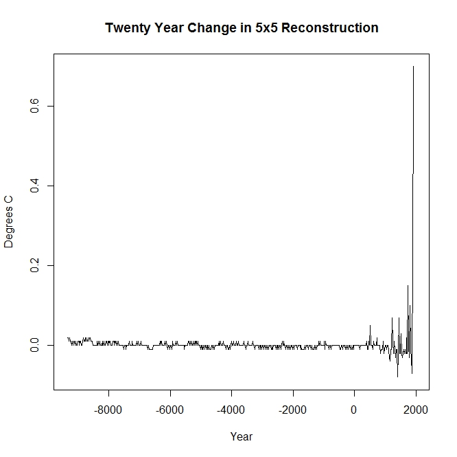
So far, the focus of the discussion of the Marcott et al paper has been on the manipulation of core dates and their effect on the uptick at the recent end of the reconstruction. Apologists such as “Racehorse” Nick have been treating the earlier portion as a given. The reconstruction shows that mean global temperature stayed pretty much constant varying from one twenty year period to the next by a maximum of .02 degrees for almost 10000 years before starting to oscillate a bit in the 6th century and then with a greater amplitude beginning about 500 years ago. The standard errors of this reconstruction range from a minimum of .09 C (can this set of proxies realistically tell us the mean Temperature more than 5 millennia back within .18 degrees with 95% confidence?) to a maximum of .28 C. So how can they achieve such precision?
The Marcott reconstruction uses a methodology generally known as Monte Carlo. In this application, they supposedly account for the uncertainty of the proxy by perturbing both the temperature indicated by each proxy value as well as the published time of observation. For each proxy sequence, the perturbed values are then made into a continuous series by “connecting the dots” with straight lines (you don’t suppose that this might smooth each series considerably?) and the results from this are recorded for the proxy at 20 year intervals. In this way, they create 1000 gridded replications of each of their 73 original proxies. This is followed up with recalculating all of the “temperatures” as anomalies over a specific 1000 period (where do you think you might see a standard error of .09?). Each of the 1000 sets of 73 gridded anomalies is then averaged to form 1000 individual “reconstructions”. The latter can be combined in various ways and from this set the uncertainty estimates will also be calculated.
The issue I would like to look at is how the temperature randomization is carried out for certain classes of proxies. From the Supplementary Information:
Uncertainty
We consider two sources of uncertainty in the paleoclimate data: proxy-to-temperature calibration (which is generally larger than proxy analytical reproducibility) and age uncertainty. We combined both types of uncertainty while generating 1000 Monte Carlo realizations of each record.
Proxy temperature calibrations were varied in normal distributions defined by their 1σ uncertainty. Added noise was not autocorrelated either temporally or spatially.
a. Mg/Ca from Planktonic Foraminifera – The form of the Mg/Ca-based temperature proxy is either exponential or linear:
Mg/Ca = (B±b)*exp((A±a)*T)
Mg/Ca =(B±b)*T – (A±a)
where T=temperature.
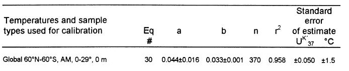
For each Mg/Ca record we applied the calibration that was used by the original authors. The uncertainty was added to the “A” and “B” coefficients (1σ “a” and “b”) following a random draw from a normal distribution.b. UK’37 from Alkenones – We applied the calibration of Müller et al. (3) and its uncertainties of slope and intercept.
UK’37 = T*(0.033 ± 0.0001) + (0.044 ± 0.016)
These two proxy types account for (19 (Mg/Ca) and 31 (UK’37)) 68% of the proxies used by Marcott et al. Any missteps in how these are processed would have a very substantial effect on the calculated reconstructions and error bounds. Both of them use the same type of temperature randomization so we will examine only the Alkenone series in detail.
The methodology for converting proxy values to temperature comes from a (paywalled) paper: P. J. Müller, G. Kirst, G. Ruthland, I. von Storch, A. Rosell-Melé, Calibration of the alkenone 497 paleotemperature index UK’37 based on core-tops from the eastern South Atlantic and the 498 global ocean (60N-60S). Geochimica et Cosmochimica Acta 62, 1757 (1998). Some information on Alkenones can be found here.
Müller et al use simple regression to derive a single linear function for “predicting” proxy values from the sea surface temperature:
UK’37 = (0.044 ± 0.016) + (0.033 ± 0.001)* Temp
The first number in each pair of parentheses is the coefficient value, the second is the standard error of that coefficient. You may notice that the standard error for the slope of the line in the Marcott SI is in error (presumably typographical) by a factor of 10. These standard errors have been calculated from the Müller proxy fitting process and are independent of the Alkenone proxies used by Marcott (except possibly by accident if some of the same proxies have also been used by Marcott). The relatively low standard errors (particularly of the slope) are due to the large number of proxies used in deriving the equation.
According to the printed description in the SI, the equation is applied as follows to create a perturbed temperature value:
UK’37 = (0.044 + A) + (0.033 + B)* Pert(Temp)
[Update: It has been pointed by faustusnotes at Tamino’s Open mind that certain values that I had mistakenly interpreted as standard errors were instead 95% confidence limits. The changes in the calculations below reflect the fact the the correct standard deviations are approximate half of those amounts: 0.008 and 0.0005.]
where A and B are random normal variates generated from independent normal distributions with standard deviations of 0.016 0.008 and 0.001 0.0005, respectively.
Inverting the equation to solve for the perturbed temperature gives
Pert(Temp) = (UK’37 – 0.044)/(0.033 + B) – A / (0.033 + B)
If we ignore the effect of B (which in most cases would have a magnitude no greater than .003), we see that the end result is to shift the previously calculated temperature by a randomly generated normal variate with mean 0 and standard deviation equal to 0.016/0.033 = .48 0.008/0.033 = 0.24. In more than 99% of the cases this shift will be less than 3 SDs or about 1.5 0.72 degrees.
So what can be wrong with this? Well, suppose that Müller had used an even larger set of proxies for determining the calibration equation, so large that both of the coefficient standard errors became negligible. In that case, this procedure would produce an amount of temperature shift that would be virtually zero for every proxy value in every Alkenone sequence. If there was no time perturbation, we would end up with 1000 almost identical replications of each of the Alkenone time series. The error bar contribution from the Alkenones would spuriously shrink towards zero as well.
What Marcott does not seem to realize is that their perturbation methodology left out the most important uncertainty element in the entire process. The regression equation is not an exact predictor of the the proxy value. It merely represents the mean value of all proxies at a given temperature. Even if the coefficients were known exactly, the variation of the individual proxy around that mean would still produce uncertainty in its use. The randomization equation that they should be starting with is somewhat different:
UK’37 = (0.044 + A) + (0.033 + B)* Pert(Temp) + E
where E is also a random variable independent of A and B and with standard deviation of the predicted proxy equal to 0.050 obtained from the regression in Müller:
The perturbed temperature now becomes
Pert(Temp) = (UK’37 – 0.044)/(0.033 + B) – (A + E) / (0.033 + B)
and again ignoring the effect of B, the new result is equivalent to shifting the temperature by a single randomly generated normal variate with mean 0 and standard deviation given by
SD = sqrt( (0.016/0.033)2 + (0.050/0.033)2 ) = 1.59
SD = sqrt( (0.008/0.033)2 + (0.050/0.033)2 ) = 1.53
The variability of the perturbation is now three 6.24 times as large as that calculated when only the uncertainties in the equation coefficients are taken into account. Because of this, the error bars would increase substantially as well. The same problem would occur for the Mg/Ca proxies as well, although the magnitudes of the increase in variability would be different. In my opinion, this is a possible problem that needs to be addressed by the authors of the paper.
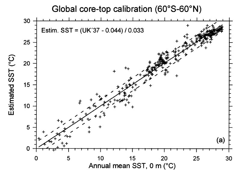
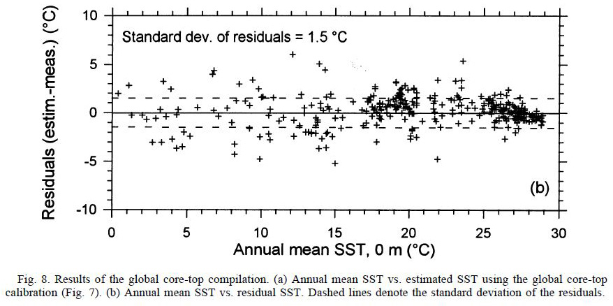
The regression plot and the residual plot from Müller give an interesting view of what the relationship looks like.
I would also like someone to tell me if the description for ice cores means what I think it means:
f. Ice core – We conservatively assumed an uncertainty of ±30% of the temperature anomaly (1σ).
If so, …


264 Comments
Ultimately we are interested in the uncertainty between the result of the calculation and the actual temperature. In statistics we infer this kind of error from the sample variation which is usually a reasonable assumption. But what happens to this assumption when you start to use a Monte Carlo method to bulk up your sample?
To give an extreme example, suppose that only one proxy measurement was input into the procedure. The Monte Carlo method would then inflate this to a respectable looking sample of 1000 data points. The variation of this respectable looking sample could then be accurately computed, but in fact it would tell us absolutely nothing about how far away we are from real temperatures. You can’t manufacture certainty out of nothing.
I confess that I have not time to read Marcott’s paper to see how this issue was addressed.
Re: Ian H (Apr 4 20:19),
Agreed. I had assumed they had used a polynomial fit of order N+1 to connect N points. But to connect them with straight lines? This results in infinite acceleration in the rate of temperature change at each of the data points. Hardly a good starting point if you are trying to improve resolution.
My initial impression was the same as Ian’s. But then I thought nothing that crazy could get published. Perhaps it could? Is this in essence what they have done?
You want to estimate the mean height of the male population of a town. You sample 73 people. Write down their heights. You then perturb each of them by generating a normal realisation with standard deviation 1sigma (As far as I can see, the value for sigma is the sample standard deviation of the 73). Now repeat this 1000 times. This gives you 1000 estimates, each based on a “sample” size 73. Take the average of your 1000 estimates as your estimator of the town’s mean male height and use the sample standard deviation of this “sample” size 1000 as your error estimate.
As Ian says, you cannot erradicate bias by generating more data points from the original ones. Also, you cannot increase precision. To see this, imagine 10 million new estimates, rather than 1000. The standard deviation of the resulting estimate would very close to that derived using the original 73, but cannot be lower. However, if you treated this as 10 million times 73 sample points of actual heights, the standard deviation of the resulting estimate would be very close to zero.
OK, there are no towns population 73 million. Assume the sampling is “with replacement”. i.e. men can be measured more than once.
I think what I am trying to say is an abstracted illustration, applied to a simple problem, of Steve’s post starting from
So what can be wrong with this?……
Nice example. However, it seems to me Marcott et al measured the height of all people – young, mature, old, men, women, from the Netherlands, Vietnam, West Africa, etc. That E term looks bigger and bigger.
Also I am pretty sure that they perturbed on the timing of the temp measures not the temp measures themselves. In the paper they say they used a 1C proxy uncertainty. This seems low compare to Muller’s estimate for Alkenones.
It sounds like they are trying to move the points on the proxies around to see if they can get then to “line up”, and then when they have the best fit between the proxies they call this the actual signal.
However, this approach ignores the obvious fact that these proxies are regional and we know that different region do not move in unison. Often when it is hot one place it is cold in another – for example the polar see-saw.
Rather than improving the resolution in this case it would just as likely tend to create nonsense, as it tried to shift the points around forward and backward in time to try and invert one proxy to match the other. This could result in high temps being shifted in one direction and low temps in the other and create trends where there were none.
My initial thoughts on this technique is that it might work with multiple proxies from a similar location to reduce error, but over widespread area it could be poorly behaved because the underlying assumption is wrong. There is nothing to say that the proxies from different regions should be expected to move in unison, have similar magnitudes, or even move in the same direction.
I’m very strongly reminded of the tree ring calibration problem. I wonder if this isn’t another example of selection bias? In effect they are using the “average” temperature of the proxies to select which proxies to use. The proxies that stray from the “average” are adjusted to match the average – in effect they are de-selected through adjustment. There appears to be a huge opportunity to introduce (amplify) error.
Would someone assist? Tamino has put in some artificial spikes to show that these would be detected using Marcott’s methods (I think) and as such spikes are not seen anywhere in Marcott’s reconstruction but are seen in the grafted temperature records for the 20th century, he concludes that it is only in the 20th century that such marked increases have occurred in an 11500 year time span. Because I’m banned from Tamino’s site for arguing and generally not showing sufficient obeisance I can’t ask if the proxies for the 20th century show this spike. I understand that there are problems using recent proxies, I don’t really know what they are but if one can artificially insert spikes in earlier periods of the time frame studied to see if they can be detected it might be informative to see if such spikes are in fact present by determining temperature in the 20th century using proxies rather than instrumental measurements. Apologies in advance for my obvious ignorance, my area of scientific expertise is biochemistry not climate science
Ian, Physicist Clive Best says he has debunked Tamino’s last post (looks plausible though I can’t judge). Also notes that Tamino has blocked him! The notorious “open mind” of Grant Foster aka Tamino strikes again….
Re: Ian (Apr 4 20:24),
Tamino and RC have been excited ever since I posted this article at their web-sites:
“as such spikes are not seen anywhere in Marcott’s reconstruction but are seen in the grafted temperature records for the 20th century, he concludes that it is only in the 20th century that such marked increases have occurred in an 11500 year time span.”
I don’t think that’s his reasoning. He says elsewhere that the proxies are particularly unable to resolve 20th Cen, because of declining numbers and end effects. But we know there was a spike (CRU), and he’s saying that a spike like that would have shown up in the earlier record.
Again, there is a spike in instrumental data but it has never been detected by a reasonable proxy. This is very annoying.
“he’s saying that a spike like that would have shown up in the earlier record”
But there was at least one such spike, though a cold one, the 8.2 KA event, and it doesn’t show up.
Nick: As I understand it, no spike equivalent to the 20th century would show up in the proxy record because of the low resolution of the proxy record, right? I seem to remember reading about a 300-year resolution, though perhaps some proxies are better than that?
Wayne,
300 year was supposed to be the upper limit – yes, many are better. But even though they might not show up well in individual proxies, when you average 73 there is a better chance. I haven’t done the calc myself.
Wayne
Source: Revkin’s interview of Jeremy Shakun at Dotearth April 1
Nick: “when you average 73 there is a better chance”.
Two comments: 1) “better chance” is no a very reliable method, and 2) averaging tends to smooth so I’d say averaging 73 items makes it less likely.
And as David L Hagen says below, there’s nothing in the data that can show anything less than 300-year-cycles. No amount of statistical processing will pull out spikes of 50 years. None.
What you have is centuries of highly-smoothed data followed by a half century of barely-smoothed (because there’s not much) data. That will make a hockey stick every time. Try it yourself.
Re: Ian (Apr 4 20:24),
Tamino has played a magician’s trick on you. He hasn’t added the spikes to the location where the proxies were created, he has drawn them on top of the proxy data. To understand this by analogy, consider this:
Adding additional planets around stars does not make them detectable to astronomers 50 years ago. These additional planets would be real spikes. However, drawing picture of planets on the old photos will certainly make them detectable! These are Tamino’s spikes. Your half blind old granny could detect them!! So, no surprise Marcott was able to do the same.
Re: Nancy Green (Apr 4 21:25),
Nancy, I like your analogies. I believe you’re exactly correct about “drawing pictures of planets on the old photos.”
Here’s approximately how I put it to Tamino in a blocked post, and also on Clive Best’s:
(I created a comment for Tamino pointing out two apparent flaws in his analysis, and suggesting workarounds. He’s not released it…)
To a person familiar with how data works it is visually obvious that Tamino’s methodology has a problem. One vs 100 vs 1000 perturbations in his method produce almost identical spike results, but with ever-smoother background data.
I believe Roman’s analysis provides a mathematical background for why Marcott AND Tamino’s methods simply don’t work. In essence, they are oversharpening the data, and in Tamino’s case he’s oversharpening an introduced digital defect.
1) Real world data would never introduce exactly identical spikes in X (time) and Y (amplitude) in all 73 proxies. Doing so introduces what is essentially a digital defect in the data… the same as an artificial dropout, or a scratch on a CD (or in Nancy’s analogy, a painted-on planet 🙂 )… When it is so perfectly aligned in the raw data, the defect will naturally survive a wide variety of processing algorithms. Yet this is what Tamino did. In the real world, different proxies will reflect climate in different ways, with at least slightly different temperature responses (assuming they are all temp proxies!) Even real thermometers don’t all produce the exact same signal.
Tamino should have had proxy-dependent variability, as well as some level of randomness, in his spike-production method.
2) Tamino’s methods are not fully explained with respect to perturbation and time-adjustment (end cap)… Steve M showed that the decisions underlying those methods and parameters are crucial to whether a spike even shows at all in modern times.
Now RomanM shows how the original Marcott method over-sharpens the data.
My final thought: IIRC, the strange thing about the “spike” in Marcott is that it is not seen in the unprocessed raw data. By whatever means, the spike is a feature of the processing methods and parameters. Yet these simulations of paleo “spikes” involve introducing raw-data spikes and determining whether the processing will eliminate the spikes. Seems like inverted tests to me!
I’m sensing two questions are important:
a) If there were temp ‘spikes’ in the past, would they be visible
b) How likely is it that processing methods and parameters will produce a spike that’s not in the original data?
Re: MrPete (Apr 4 22:06),
I’m sensing two questions are important:
a) If there were temp ‘spikes’ in the past, would they be visible
==========
As per my more detailed analogy, they would only be visible if the resolution of the proxy is sufficient to make them detectable. You can study the old photo’s of other stars all you want and you will never find a planet – unless “Tamino” has drawn one in. Yet newer, high res techniques now make it appear that planets are quite common.
A) Yes, but only if they were originally large enough to pass through the filtering process. They would be heavily attenuated from their original form. Furthermore, depending upon circumstances, they might not resemble their original form.
B) Zero, unless the processing method was designed to do so. Legitimate processing techniques, implemented correctly, should never add information, they should only make existing information easier to analyze.
Mark
It is quite easy to figure out, how “real world data” would if represented by such proxies.
With a 300 years resolution, data of +-150 years would be averaged. Temperatures from 1863 +-150 years would then contain data from the little ice age as well as from today averaged in one data point.
On top of this there are dating errors when combining different proxies, leading to a further spread of averaged data in use and a further loss of variation.
On top of that such proxies do not represent only temperature but various other related and unrelated variables which will contribute to a further loss of variation.
So their use of Monte Carlo allowed them to have smaller error bars thus giving the impression of greater confidence/accuracy. The more I hear/read the more I believe everything they did was to produce a specific result. GO TEAM!
Great stuff here Roman. Leaving the prediction error out of the Monte Carlo model? Tsk. And of course the assumptions of the Muller et al calibration model (and any associated variance attenuation) are also imported into Marcott’s reconstruction as well. Then of course we have the uncertainty of the offset alignment with modern temperatures. This could take a while.
This is the second time you have dropped a comment on this matter. You wouldn’t by any chance be planning to take a closer look at this now would you? 😉
Roman:
This is very elegantly and clearly stated.
Have you looked at Nick Stokes tool that allows you to visualize all the proxies? I am not sure technically how it relates to your analysis above but the lack of variance of the proxy anomalies particularly between roughly 5000 and 7000 BP looks very strange especially given Figure 8 that you very helpfully pasted into your post and the SE of +/- 1.5C.
I would like to see what the error bars would look like if done correctly!
Scott,
I expect that you would not see them assuming you kept the y-axis constant. 😉
Roman M,
I’m not following your logic here.
Assume no autocorrelation.
If I fit a model with residual error, E, I can generate realisations from the model by predicting mean model values and sampling from E; OR I can sample from the coefficient distributions and set E to zero. If I allow both the coefficients and the residual error to vary for each realisation then i will end up with an overestimate of the error variance. No?
Muller’s coefficients were a fit to the mean. The actual observations (actually residuals) are distributed about the mean with a SD of 1.5C. Where is that accounted for?
I don’t believe that is necessarily the case here. The model estimates are calculated from one sample and then the predictions are made on a data which are external to that sample. The error in the coefficients is independent of the E for the data to which the prediction is applied. You are dealing with two independent sources of uncertainty and both are playing a role. There is also a second step in which one has to solve for the “temperature” perturbation which does make the situation more complicated. I am willing to be convinced that you are right if you can come up with a good argument.
Either way, I don’t think that what was done by Marcott is correct.
Roman,
I commented below that I just couldn’t understand why you’re adding in a measure of Muller’s residuals (which I presume is E). I still can’t, but it seems now to me that you might be doing so because M did not include varying UK37 according to its uncertainty. It surely wouldn’t make sense to include both.
Just looking at your math, I think your first equation should actually be
U=0.044+A+(0.033+B)*(T+δT)
where U=UK37, δT=Pert(Temp)
Then to first order, we’ve created a random variable
δT=(-A-T*B)/0.033 (differs from yours by T*B)
But then you take mean of 1000. That should make the change very small, otherwise 1000 is not enough. The only thing of interest should be the mean of product terms. And here, I suspect that is very small too.
You want to add in E. The only way I can make sense of that is as a proxy for δU – uncertainty in UK37. But again, just adding that should leave no net change after mean of 1000.
Incidentally, I presume A and B are independent of time. It wouldn’t make much sense to think of the interpolation formula varying randomly from one time to the next. In that case, any effect they did have is likely to vanish after taking anomalies.
It seems to me that it’s only perturbing the age model that does anything interesting.
You are correct on the first part, but wrong on the second. Yes, the E is due to the fact that even if the regression line predicting proxies from temperature is known exactly, the observed proxies will not all fall exactly on the regression line. The uncertainty due to the fact that the regression coefficients are not known exactly contributes uncertainty independently of E. Saying that it wouldn’t make sense to account for both is statistically naive.
In fact, both are taken into account in a much less clumsy fashion than varying coefficients as done in Marcott et al when one calculates prediction intervals in regression. Müller does not overtly give enough information on the observed temperatures used in the regression (one needs the means and variance of those temperatures) to do the exact calculation and I am not sure whether I can infer them from the information given. However, if you look at the formula for the prediction interval, you will see that the end result has a lower bound of the standard deviation of E. This also addresses your point that changing the coefficients each time because those values do not appear overtly and it also deals with the fact that I was ignoring the effect of the variation of the slope coefficient in my post.
I will add an update to my post on this approach when I get a chance later today.
Nick: Obviously Roman can answer best, but I haven’t seen these particular words. There are two variances around a central value involved: 1) The variance that reflects your uncertainty in calculating a parameter of your model, and 2) the variance of the fit of the data to your model.
I believe this is the difference between the SD of our data and the SE of our slope and intercept. Even if we know, a priori what the slope and intercept are (SE’s are zero), that does not mean that the data will fall directly on the line (SD is not zero). Both sources of variability must be accounted for, but most of the time all we focus on are the SE’s.
[Roman: This is exactly what I am saying but you have expressed it in more technical terminology. I have been using simpler language so that people who do not have a sufficient statistical background can get the sense of what is wrong with the Marcott approach.
Roman: Yes, it’s best to explain things at the appropriate level for the audience and I think you’ve done well.
This kind of discussion really hurts my head, though. On the one hand, it makes me want to step through the whole chain of analysis from measurement to result, looking at the uncertainties at each step. And there is a LOT of uncertainty/variability that is not usually carried forward through that chain that should be. A LOT of assumptions are made and we end up with layer upon layer of abstraction and smoothing that is simply not reflected in the statement of the results.
So then I think, wow, the results we see reported are way overconfident. But then I hear some non-technical skeptics arguing that everything is so uncertain that we can’t possibly know anything so let’s just assume it’s all okay and stop poking around. No, that’s wrong, too.
And these two poles create a real tension that is just headache-inducing.
It feels like science is devolving into four camps: 1) scientists who gather data but then keep it close to the vest because knowledge is power, 2) scientists who are enamored with statistical methods and so take whatever data is at hand and assume if they use sophisticated-enough statistical methods they will get legitimate answers — better answers than the data would seem to support — but then 3) lay people who assume what’s “peer reviewed” or what uses “sophisticated statistical methods” must be right, and 4) lay people who are skeptical of science overall.
It’s a sad state, really. Though maybe I’m biased because the climate field is the poster child for enamored-with-statistics. (I don’t mean to imply that I’m a climate scientist, I’m not. But following this field is part of a hobby of mine so it’s over-represented in my impression of science at large.)
Steve: I think (and certainly hope) that the commentary here falls into a 5th category. The strongest commentary here applies statistical requirements to science articles that are often weakly peer reviewed.
Nick: “No, this is not regression, it’s applying a regression relation”. You need to quote what you’re replying to, since we’re all reduced to a flat thread at this depth. I assume you’re addressing my comment about errors-in-variables by saying that the x’s of which you speak (which have errors) are not being used in a regression.
I can accept that. My mistake.
(Though I’d add that it’s my impression that the original regression had errors in its x’s (time).)
Roman: You and your readers are struggling with the proper analysis of confidence interval in what an analytical chemist would call a standard curve. One can see a presentation of how an analytical chemist would do this analysis at:
Click to access 07_Calibration.pdf
The 17th, 20th and 21st slides illustrate the problem you are dealing with. If the UK’37 ratio can be measured with complete precision, you are dealing with a situation that looks like slide #21. (My guess is that the sensitivity of the alkenone proxy (95% confidence level) is understood to be about 1.1 degC, meaning that a 1.1 degC temperature change will be real 95% of the time.) Unfortunately, no measurements are ever made with complete precision. In that case you are dealing with a situation link slide #17, where the uncertainty in the calibration curve combined with the uncertainty in measuring UK’37 creates additional uncertainty (which I think you are calling E).
Frank,
“creates additional uncertainty (which I think you are calling E)”
Your slide 17 etc just deal with the algebraic consequences of the uncertainty of slope and intercept (A and B of the post). So did the prediction interval link that Roman referred me to. There is no extra E referring back to the residuals of the original regression. And I am now thoroughly convinced there should not be.
To see this, take Roman’s extreme where Muller has an infinite sample, and A and B were zero. Then your slide 17 would, correctly, be telling you that you just convert with the straight line. No extra E. The x-axis variable has uncertainty, which converts directly to that of the y variable.
I think Roman’s fallacy is the statement:
“The regression equation is not an exact predictor of the proxy value.”
Of course not, but they are not trying to predict the proxy variable. They have a reading. They are trying to predict how the proxy variable depends on T. Muller did a regression which discriminated a component that depended on T from a residual that did not. Marcott need not be concerned with the various ways in which Muller’s samples varied independently of T. He only needs the T dependence.
Nick, it seems to me that you must never have taken an elementary mathematical statistics course.
What’s the difference? They are deriving an equation which which predicts what the expected value of the proxy will be for a given temperature. As in any linear regression, Müller et al start with a linear model for the relationship between Proxy P and temperature T:
P = A + BT + E
where A and B are numeric constants. E is there from the very start to account for the simple fact that for a fixed temperature T, the measured proxy values will vary – in a scatter plot, they may appear above or below the line P = A + BT. E is assumed to be a random variable with mean 0 (which gives the line a physical meaning as the mean of all proxy values for which have an associated temperature value of T and a standard deviation of σ which describes how far the actual observed proxy value might be vertically from the line.
But A and B are not known, so the first step is to estimate them and that is what Müller did. They took 370 proxy samples along with their 370 associated temperatures and came up with estimates a, b and s for the parameters A, B and σ. The results were a = 0.044, b = 0.033, and s = 0.050. They also realized that a and b were not exactly equal to A and B, so they calculated estimates of their standard error (i.e. uncertainty) due to that pesky E term in the original model and came up with s(a) = 0.016 and s(b) = 0.001.
Now Marcott comes along with a (possibly different) set of proxies and decides that he can use this regression equation to “predict” what the temperature may have been for the conditions under which those proxies were formed. He solves for T as a function of P and gets T = (P – a)/b, thereby generating his set of “temperatures”. But, wait a minute – there was an E in that equation. What happened to it? They assumed in each case that the E was equal to 0. The effect of the variability of the proxies around the regression line has been completely lost in this process.
In order to be able to calculate error bounds for their results, they need to somehow restore this information into their data and they decide to do this by using their Monte Carlo methodology. What needs to be done is to add in a randomly generated E and see how the temperature estimate changes. However, in a very clumsy effort, they decide that perturbing the coefficients alone according to their uncertainty will do the job. It does not achieve the necessary result because it only deals with how well Müller was able to estimate the coefficients and not with the variability of predicting the proxies themselves.
This is patently false. First of all, as one can easily see from the model, E does not relate just to the “residuals of the original regression”, but to ALL of the proxies. Secondly, the prediction formula applies to proxies outside of the original study. Now look carefully at the part of the formula for the prediction interval under the square root. The initial “1” is E. Statisticians are clever people. 😉 They figured out that the distribution of the distance from a new proxy value from the calculated line is a (multiple of a) t distribution with n-2 df (368 in this case – read “normal” for that many df) with mean zero and with standard deviation equal to s*(the square root part of the formula). This takes into account E AND the uncertainties of a and b and this is the perturbation amount that should be applied to the proxy.
By the way, if you remove that “1” from the equation, you get what is needed to calculate a confidence interval for the line itself.
[Update: The link to the prediction interval is this.]
Nick Stokes (Apr 6 03:33),
I’m struggling to understand your point. In their MC perturbation analysis Marcott et al only accounted for the “model uncertainty” (Frank’s slide 13), i.e., calculated their “proxy-to-temperature uncertainty” by estimating the mean response SD. Are you saying that it is the correct approach?
Jean S,
My point? Roman says there is a big omission in Marcott’s MC which is E:
“E is also a random variable independent of A and B and with standard deviation of the predicted proxy equal to 0.050 obtained from the regression in Müller”
As far as I can see, E is effectively the residual in the original regression
UK’37 = (0.044 + A) + (0.033 + B)* Pert(Temp) + E
“Even if the coefficients were known exactly, the variation of the individual proxy around that mean would still produce uncertainty in its use.”
I do not believe those residuals need to be considered. Here’s a thought experiment. Suppose there was another independent variable s affecting UK37, not interacting with T. s normally varies with no detectable pattern, so it’s effect is included in noise. But suppose in Muller’s situation, the amplitude of s variation was unusually large, so he had to compensate by taking a lot of samples. Does Marcott have to take on an error term for that s variation?
In any case, no such reference to a third independent variable appears in Frank’s slides, as I far as I can see. There is only the uncertainty in the regression coefficients, which Narcott allowed for.
What do you think would be the value of E in the case where A and B are very small?
Nick Stokes (Apr 6 06:40),
you didn’t answer my question. I’m not interested in “thought experiments”. I gave you a link which as far as I understand is precisely dealing with the situation. Please formulate your point in terms of the link, and this might actually lead somewhere.
Jean S,
Yes, I believe mean response is the right thing for them to use. But this is a somewhat different question. Roman is talking about importing a variable from Muller’s regression.
The reason why I think the mean response is right is because of its role in the Monte Carlo. There isn’t any point in just adding variation to the observed variable, because the Monte Carlo averaging will simply remove it with no residual effect, assuming there are enough repetitions.
Nick Stokes (Apr 6 07:27),
Thanks, Nick! We now know precisely what we disagree on. And knowing your ways for many years, I do not even try to convince you of believing anything else.
Yes, that’s precisely what makes the difference between the mean and predicted responses in their perturbation analysis.
Nick –
I must be missing something here. The residual error in Muller’s sample regression has a SD of 1.5 K. That represents a lower bound on the accuracy of the temperature attributed to a given sample.
Suppose that, in digging in the muck, we didn’t find proxies but readouts from a digital thermometer (naturally it will have a date stamp such as 3456 BC ;-). Being a primitive digital thermometer, it had a relatively poor accuracy of +/-1.5 K (1-sigma). Averaging N of these readings will result in a metric T0 which ideally has a mean value of the actual temperature, but a SD of 1.5K/sqrt(N). For N=73, that means SD ~= 0.2 K. That value constitutes a lower bound on the Marcottian uncertainty. [Well, not quite — not all Marcott proxies are alkenones and I don’t know the SDs of the other proxy types.]
HaroldW
“I must be missing something here.”
Well, I guess one of us is. It’s late here, but it’s the night when we leave daylight saving, so I guess I have an extra hour. It may not make me wiser though 😦
That 1.5°S is just 30x the (Muller) UK37 se – 30 is inverse regression slope. I think here too, the primary uncertainty in T is 30x the uncertainty in their observed UK37, whatever that is.
I’m not sure what to make of the bronze age digital thermometer; it’s UK37 that is dug up. In fact I believe the real error source is not in the UK37 obs itself, but where and when it came from.
Jean S,
“And knowing your ways for many years, I do not even try to convince you of believing anything else.”
Well, I may be incorrigible, but I’m sure there are more perceptive listeners who will be interested.
Nick,
I realize that this is an argument from authority, but the odds of you being correct on a statistical issue as opposed to Jean S and Roman, is as low as Mann’s verification r2. You’re arguing here with specialists within their specialty
Nick: “The x-axis variable has uncertainty” If this is true, OLS does not work properly. You need to go to an Error-in-Variables kind of approach.
Jean S,
You are not effusive in your explanation, and I think I may see a crossed wire. I have been talking of the Monte Carlo which produced the mean curve after date variation etc. I see that you may be thinking that Marcott et al used that as their sole source of error bounds for the curve. That would indeed be wrong, but I don’t see that stated in either paper or thesis.
While I’m not in possession of the Muller et al. paper, this is speculative, but the SE in UK37 of 0.05 appears not to be uncertainty (which in this case I take as measurement uncertainty), but the spread on observed values at sites with the same SST. The SE of the estimated SST, at 1.5 K, is (as you say) 30 times that value, being just the result of solving for T from the observed UK37 values through the equation UK37 = 0.044 + 0.033*T. The meaning is still that, using the Muller best-fit coefficients, the estimated T differs from the actual by +/-1.5 K, as the second panel of figure 8 indicates.
Thinking about this some more, varying the A coefficient should have no bearing at all on the reconstruction, as the anomalization step (4500-5500BP) will negate this. Unless Marcott varied A for each sample independently, which would not seem to be consistent with its meaning as a calibration coefficient.
Wayne2,
No, this is not regression, it’s applying a regression relation.
But on the question of how M et al derive their blue CI’s; following through their Fig S2 and explanation, they aggregate in step c over the 73 proxies, and record a standard deviation. I assume that includes the between-proxy variance as well as the Monte Carlo variances, which if they were all of the same kind, would be where uncertainty in UK37 (or equivalent) values is included.
RomanM (Apr 6 08:20),
nice and very throughout explenation! But I’m afraid you are wasting your time with Nick (hopefully the explenation is useful for other people). He already stated that he believes that it is enough to account only for the errors in A and B…
Roman,
Their UK37, in your terms has a component depending on temperature (mean response) and a component that varies with other things. In compiling their stack, they account for error in the mean response through the Monte Carlo. But they include in their variance (I believe) in step c, Fig S2, the between proxy variance over their 73 proxies. Is this not covering your E? The variance in proxy values due to non-temperature effects?
Why are you still up? I thought you were going to bed! 😉
In their paper, Marcott et al keep referring to “the chronologic and calibration uncertainties estimated with our Monte Carlo simulations”. This procedure is crucial to their calculation of calibration effect on the end result. The contribution of these particular proxies that constitute 68% of all proxies used toward estimates of the error bars is very substantial. Imagine the spaghetti graph S3 in the supplement being two or more times as wide. Depending on how many replications are done, there could very well be higher variability in the reconstruction as well. In my view, correcting their work would make real substantial changes in the paper and this has to be addressed by the authors.
As an aside, there is also a slight upward bias introduced by the perturbation of the slope coefficient, but that is another issue.
Roman, Jean,
To put my argument there another way – suppose they didn’t vary dates. Suppose they didn’t vary the regression coefficients. Supposed they reduced their Fig 2 process to just step c, averaging over the 73 proxies and using the (weighted) sd to construct the CIs. Do they need your E as well?
Nick Stokes (Apr 6 09:23),
I don’t see any such step on p.8 (SI), where they explain the procedure. CIs are calculated in the step 6).
Jean S,
Yes, I think it is in step 6, They say “The mean temperature and standard deviation were then taken from the 1000 98 simulations of the global temperature stack (Fig. S2d),”. That’s the step, shown in Fig S2, where they take the area-weighted mean over the 73 proxies. I assume the sd they refer to includes the variance over those proxies.
That’s not the way I read it. Step 5 says:
To me, this indicates that 1000 reconstructions were created from the simulations in Step 5 which were then averaged to form the overall reconstruction and to calculate the standard deviation(s?). I don’t see this as referring to “variance over those proxies” in any way.
Nick Stokes (Apr 6 10:18),
what? Are you suggesting that their SD includes also proxy variance over time or over different proxies? That would be crazy, but I don’t see anything like that going on but only variance over 1000 (mislabeled 10000 in the figure as in the thesis) “stack” realizations (as it should).
And I think Nick Stokes’ fallacy is the statement :
“Argumentum ultimum verbum.”
If your model is: P = A + BT + E
then I suspect your A and B should be exact numbers.
If your model is: P = (A+/-dA) + (B+/-dB)*T
then I suspect you don’t need an E term. The curved confidence intervals around the linear regression provide a nice graphic representation of how uncertainty transfers from the temperature axis to the UK’37 axis and back. However, one needs to recognize that there may be significant experimental variability (dP) in measuring P (which potentially can be reduced by analyzing multiple samples). The uncertainty in P must be transferring to the temperature axis as shown in overhead #17). Rearranging gives
T = [(P+/-dP)/(B+/-dB) – (A+/-dA)]/(B+/-dB)
The model for the regression in Müller is P = A + BT + E. The people applying the result to their proxies have assumed that a single A and single B is used for all proxies from all locations.
Don’t confuse estimation uncertainty (which is not part of the model definition) with something like modelling the variation in the proxy-temperature relationship (which should be part of the model).
For example, I might wish to model the situation that intercept and slope might be related to physical location of the proxy site. In that case, my model equation might look like
P = (A + dA) + (B + dB)*T + E
where dA and dB are extra parameters and E = dP in your statement. The statement of a model should contain all of the relevant assumed features of the situation including any sources of randomness – your model specification should have had it written in rather then added on as an afterthought.
Jean S,
“Are you suggesting that their SD includes also proxy variance over time or over different proxies?”
Over different proxies. If you look at their cube in Fig S2, the dimensions are age, proxies and Monte Carlo reps. They collapse to 1D by averaging over proxies and Monte Carlo. It would be logical if the sd they quote is the variance associated with this total averaging process.
Anyway, I’ll try to test today using my emulation program, which basically collapses a 2D version (no MC).
Oh, Nick! You have got to be kidding! Please stop making things up.
The description of Fig. S2 states:
Where does it say “proxies” anywhere in the description? Where do you see “proxies” in the diagram?
Even if the proxies were to be included, how would that be done? Average all 1001 series together or do you envisage they did something weird and wonderful but somehow just forgot to tell us about it?
Roman, what exactly are the “datasets” if they are not the data of each individual proxy? Or are you distinguishing between the proxy (the record of d18O, etc) and the datasets (the calculated temperature based on the proxies)?
I am not distinguishing between proxy measurement and “temperature”. Each of them carries the same information because there is an exact relationship linking the two and one is reproducible from the other..
The datasets are formed by adding randomly generated quantities to each proxy and to each time with which that proxy has been linked. Although the datasets have been calculated using real proxy and time values, they do not contain the same information.
Romanm,
‘Where do you see “proxies” in the diagram?’
Vertical axis, “datasets” #1:73
Each age value is found by averaging a 73*1000 array of proxy/MC values. I don’t see why the sd quoted would not be the sd of the numbers in that array.
What are “proxy/MC” values. They are either one or the other. Once the random elements are added to the proxies, they are no longer “proxies”. They do not create 1000 NEW proxies.
The description clearly reads: “(b) Three dimensional matrix of each of the 1000 simulated datasets.”.
Did they somehow substitute “simulated data” for “real proxy data” somewhere between (a) and (b) and then put it back before the statistics were calculated in (d).
The simulated data was merged together on the horizontal level (probably quite differently) for each of the many types of reconstructions. It then makes sense that you have 1000 values for each of the 20 year periods from which the standard deviation can be calculated.
It does seem to me that it all turns on what is meant by “perturbing them with analytic uncertainties in the age model and temperature estimates” in the Real Climate Q&A
“4. Used a Monte Carlo analysis to generate 1000 realizations of each proxy record, linearly interpolated to constant time spacing, perturbing them with analytical uncertainties in the age model and temperature estimates, including inflation of age uncertainties between dated intervals. This procedure results in an unbiased assessment of the impact of such uncertainties on the final composite.”
In both cases did they include the full prediction interval or just a subset such as confidence intervals on the coefficients. Note the different language used between the two parameters “age model” and “temperature estimates”.
Anyway my feeling is I can’t tell from the descriptions and I can’t replicate to test. I do think that Nick Stokes’ suggestion somewhere above that it all comes out in the wash when we move from point estimates to regional and global estimates is a diversion – if the variance in the point estimates is understated and a function of proxy type then averaging these doesn’t fix it.
I’m also unclear why they went through the process of perturbation on temp and date separately and then interpolated a new “sample” value, and didn’t just go there directly to find a range of points in temp-time space around the original estimate.
It was done under the principle that a good way to estimate true variability of a reconstruction would be to start by doing many identical, but independent reconstructions. Then one could average these reconstructions to estimate the temperature and calculate the standard error at each point of the reconstruction to determine error bounds. This is similar to estimating the mean of a population from an average, but then needing to compare each of the observations to that average to determine how well the average may estimate that mean.
One of the reasons for the development of Monte Carlo methods was for estimating the variability of statistics for which the standard error could not be calculated theoretically because of the mathematical complexity of the statistic. It involved creating simulated samples with the same characteristics as the original sample and then calculating the statistic for each of these. The whole point of this post is that the method used by Marcott for Alkenone proxies (and likely some others) did NOT generate “temperatures” with the same characteristics as the original sample because the simulated values lacked a component of variability which made the new values considerably less variable. The end result would be a serious underestimation of the error bounds of the reconstruction.
Roman,
“What are “proxy/MC” values. They are either one or the other. Once the random elements are added to the proxies, they are no longer “proxies”.”
I think this is quibbling. They have for each age an array of 73×1000 data points. Each row of 1000 consists of perturbations of the observed values from one proxy. When you average over the 73000, and take the sd of the 73000, you incorporate essentially all of the proxy to proxy variation. And that incorporates a good measure of proxy uncertainty. If they were of exactly the same kind, it would be the obvious measure to use. And the heterogeneity doesn’t really change that.
And this relates to HAS’s point. It’s important because if that does cover proxy age value variability, and I think it does, then it would be a bad mistake to then include E as well. Double counting.
It appears that the conversation with you is pretty much done. You do not seem to be familiar with even the most basic elements of mathematical statistics and the interpretation of regression procedures.
The difference between proxy and “perturbed proxy” is not quibbling. You don’t “average over the 73000, and take the sd of the 73000” – again you don’t seem to understand the details and the details are important – and how you understand without any previous analysis or experience that “you incorporate essentially all of the proxy to proxy variation” or how “that incorporates a good measure of proxy uncertainty” is absolutely incredible. Perhaps you could explain to us the mathematics behind how this is done.
The method for perturbing of the ages is considerably different from the method for perturbing the proxy values:
How does this affect the categorical statements you are throwing around in you comments?
On several occasions, I have explained the technical and mathematical aspects of the proxy perturbations to you. You responded every time with nothing but an opinion. Bring some real evidence to substantiate what you say and then we can have something substantial to discuss.
RomanM @ 6:34 PM
I understand why Monte Carlo, just not why they ran two Monte Carlos and then combined rather than run one in temp/time space perturbing both dimensions independently – I meant this more as a curiosity rather than a substantive point.
Nick Stokes @ 6:47 PM
Of course the point remains we don’t know whether/how much it biases the best estimate if it wasn’t done, and we know it makes a difference to its PDF.
Where did you get the idea that there were two different Monte Carlo reconstructions?
The description on p. 8 of the Supplement document indicates that they did a single one combining the two perturbations as you suggest they should.
I choked on my pinot grigio when Nick accused Roman of quibbling.
Roman,
Let me put it at it’s simplest level. Suppose the MC perturbations were small. They had 1000 rows each essentially with the same proxy numbers. And they went through the same process. They would get the same result as if they had simply taken the mean and standard deviation of the individual proxies at each age (except for area weighting, which for 5×5 has small effect). And the sd would represent the proxy spread and would be a reasonable basis for a CI.
So why does the actual MC perturbation change that? Obviously it smooths, and reduces the CI’s for that reason. But it doesn’t suddenly stop the sd from expressing proxy variability.
I have now done that calc on my original recon, which did essentially average without MC. The result was an average sd of about 1°C. Obviously a lot higher than theirs, which is more like 0.2. But theirs is very substantially smoothed relative to mine.
I’d emphasise again that the issue is not whether the inclusion of proxy variability as they do it is perfect. It’s whether it is not there at all. If it is there, then simply adding in your E is not the right thing to do.
RomanM @ 9:15 PM
From the SI:
“We used a Monte-Carlo-based procedure to construct 1000 realizations of our global temperature stack. This procedure was done in several steps:
“1) We perturbed the proxy temperatures for each of the 73 datasets 1000 times (see Section 2) (Fig. S2a).
“2) We then perturbed the age models for each of the 73 records (see Section 2), also 1000 times (Fig. S2a).
“3) The first of the perturbed temperature records was then linearly interpolated onto the first of the perturbed age-models at 20 year resolution, and this was continued sequentially to form 1000 realizations of each time series that incorporated both temperature and age uncertainties (Fig. S2a).”
Step 1) “We perturbed”; Step 2) “We then perturbed”; Step 3) we put humpty-dumpty together again.
Come to that why not carry all the distributions through the global reconstructions and do the Monte Carlo at the end and pick up the rest of noise on the way?
Nick Stokes @ 9:19 PM
Call me old fashioned but I like to start with what should have been done and compromise from there. You never know what you might miss taking the short-cut (and sometime the umpire could send you back to do it properly even if only to show the short-cut didn’t matter).
If you see what I mean.
In fact I rather suspect that in this case the short-cut that you are rationalising is really the long way round if you are really interested in what is going on.
No risk in doing it right, if it doesn’t matter it will show.
HAS,
“I rather suspect that in this case the short-cut that you are rationalising”
It isn’t a short-cut. Look at the alternative that is proposed. Estimate the variability about the regression line. Create a whole lot of artificial proxies with perturbed values. Calculate the variance. Those artificial proxies would sit on the same axis of their cube.
But how to estimate the variability? Roman says import variability from Muller’s regression. But that was done with a whole different lot of proxies and circumstances.
So use the current data? From the 73 proxies estimate how they sit around some regression lines? Create artificial perturbed proxies etc?
The fact is, we have 73 proxies which do actually have the variability we’re looking for. Why not use them directly?
It isn’t rationalising either. One who proposes adding a whole lot of variance (E) has to show that it hasn’t been accounted for already.
What I am indeed assuming, btw, is that they actually did include the whole variance from the 73*1000 points per age step. Sometimes they make it sound as if they might have taken the mean over proxies and discarded that variance, which would indeed be wrong. But they are describing a fairly sophisticated algorithm, and that would be an odd thing to do.
Nick Stokes @ 1:37 AM
But the thing I don’t understand about that approach is how you get to say anything about temperatures.
Nick (1:37 AM) –
By ignoring E one is estimating a different quantity. Let me try an analogy.
Suppose you want to estimate the average height of a population. You select a group of N=73 persons at random and look up the height on their driver’s licenses. It turns out that a previous study established that when a person of known height was measured at the dept. of motor vehicles (DMV), the recorded height was on average correct, but varied with a standard deviation of Y. With some common assumptions, you’d say something like, “the average height of this group is X +/- Y/sqrt(N)”, where X is the mean of the license heights.
Now someone comes along and tells you that the yardsticks which the DMV used didn’t go through quality control, and their markings varied. What does that do to your confidence in the average height? To assess this, you create an array of 1000 random runs, in each of which you generate a perturbed height of each person (according to the actual recorded height, and variation of the yardsticks). For each run, the mean of the N perturbed heights can be calculated. The scatter of these 1000 mean values (call it Z) is an estimate of how much the sample mean varies due to the yardstick problem: before you could say definitively that the average recorded height is X, now you say “the average height, as measured by the DMV folks, is X +/- Z”. But you can’t say that the average height is X +/- Z; you still have to include the Y/sqrt(N) factor. Although you now have 73K pseudo-heights, there are only 73 measurement errors.
Just to be clear, Roman’s E is analogous to repeatability uncertainty (deviation Y), dA & dB to the yardstick uncertainty (deviation Z).
HaroldW,
I think this analogy can be developed, but it has a difference.
1. You speak of the mean of 73 individuals (X_i). But the CIs Marcott is drawing are for the mean temperature of the Holocene. For that, the error includes sampling of the proxy readings^* from a notional population. So your analogy should be estimating a population mean, from which population the 73 were sampled. So there is the familiar problem that, without Y for now, population estimated mean is mean(X_i) and has se: sd(X_i)/sqrt(72)
2. So Y and Z are a bit much. Lets just MC Y. Add N e_j’s (N=1000, e~N(0,Y)) to each X_i and average. Then the variance(over i,j)(X_i+e_j)~variance(X_i)+Y^2/N
The MC preserves the variance of X_i in the total variance.
We still have the sample variance of X_i and have added thet due to Y.
* The “population” is complicated for the proxy analysis. It’s not the population of proxies 1:73 – we don’t have a distribution model for them. It’s really the population of residuals.
Incidentally I found a non paywall copy of Huybers and Wunsch 2004, which Marcott cites as source for the random walk etc.
HaroldW,
I tried to reply, but I think it went to spam. The gist is that I think you are looking at a mean of a sample of 73, while Marcott is showing CI’s for the Holocene temperature. So there’s a sample->population mean step that’s not in your analogy. I tried to reformulate as seeking the pop mean from which the 73 were derived. Then just one of Y and Z is enough. The MC preserves the variance of the X’s and the new Y in a combined variance, as it should.
Nick (6:01 AM) –
I don’t think the sample vs. population distinction is applicable here. Yes, there is an uncertainty due to sampling 73 points in the world, vs. the much larger number available in current thermometer averages. That’s not a limitation to my analogy; Marcott et al. don’t account for sampling error in their methodology. They discuss why they think the term is negligible in section 8 of their SI.
Time span is also not an issue. Marcott et al. do not produce a single CI for the Holocene, but a CI for each time step. Marcott’s processing, once the anomalized stacks are complete at step 4, is independent for each time step. Each element of the 1000-member ensemble (from which they determine the sample deviation) is an average of (at most) 73 terms.
Roman: I believe that P = (A+/-dA) + (B+/-dB)*T OR
P = A + B*T + E can handle the uncertainty introduced by changing location because Muller devised this relationship from data acquired from many locations. It can’t handle variability introduced by things that may have changed with time (nutrients, changing species, etc.) or the experimental variability associated with measurement of P.
In my simple way of looking at it, you have to include the E unless you believe that the model exhausts the likely variables that influence what ever aspect of the Alkenones you are measuring. Muller’s model is a gross simplification of what he is measuring. Wouldn’t Marcott et al’s actual code be helpful at this point?
Re: bernie1815 (Apr 6 09:05),
you have to include E unless you believe that your values would be exactly on the regression line given you knew the coefficients A and B perfectly (and the linear model is perfect for the relationship). I don’t know how the code would help here except for checking that they actually did what they say they did.
Nick: “But they are describing a fairly sophisticated algorithm, and that would be an odd thing to do.” Yes, yes it would be. But considering how Mann, et al, have mis-used PCA and considering that it only takes a couple of lines of R (or Matlab, or …) code to do MC sampling, I’d say that this you’re over-confident on this one.
I’ve not seen much mention of something I see hiding in RomanM’s citations… I also noticed it when I went looking for an answer to a challenge introduced over at DotEarth. I’m certainly no expert so I pose this as an observation for someone else to correct or confirm:
Some are claiming that calibration is unnecessary for these proxies because they directly reflect absolute temperature, just like a thermometer (and unlike tree rings.)
I looked for any data on the uncertainties involved in the Alkenone proxies. The only thing I could find nicely matches the data in RomanM’s post above:
The source I found (An SI posted at UMass – not sure what paper this is for!) has this to say in the figure S2 caption (p3):
Am I reading this correctly, that Alkenone proxies have an inherent temperature uncertainty well over 1 ̊C? If so, how can scientists claim that no calibration is necessary?
It seems ridiculous to say that no calibration is necessary. Any time you measure a quantity in one unit and correlate it with another you have to calibrate.
And that calibration should account for any nonlinearity in the relationship.
Even the finest platinum resistance thermocouple is a calibration between measured voltage and temperature.
What I’m curious about is that any regression used to calibrate and then to predict values of Temp should have greater uncertainty as the value of Temp moves from average Temp used in the calibration period (if I remember right). Is this taken into account – it might be significant here where it appears the hindcast values are offset from the calibration values.
MrPete
“Am I reading this correctly,”
I don’t think they are saying this is the error in the calibration formula; I think its just the underlying uncertainty in UK37 multiplied by the slope factor from the formula.
Is this something we can examine via simulation?
# Generate multiplier for error value

#err = function() { runif(1,min=-1,max=1) }

err = function() { rnorm(1,mean=0,sd=1)  }

# Convert UK'37 to temp

uk37temp = function(uk, Ea=err(), Eb=err(), Em=err()) {

    ((uk + (0.050*Em)) - (0.044 + (0.016*Ea))) / (0.033 + (0.001*Eb));

}

# 0.4351 is ODP-1019D sample 1

# No error in regression params

> sd(sapply(rep(0.4351,100000),uk37temp,Ea=0,Eb=0))

[1] 1.511062
# Marcott, no measurement error
> sd(sapply(rep(0.4351,100000),uk37temp,Em=0))
[1] 0.6042104
# All errors
> sd(sapply(rep(0.4351,100000),uk37temp))
[1] 1.634209
MrPete: The 20th and 21st overheads in the presentation I mentioned define and illustrate the sensitivity of any analytical method relying on a standard curve. It would make sense if the confidence interval you cited for alkenone proxies (+/-1.1 degC) were determined as shown for the sensitivity (from the 95% confidence intervals for the least-squares fit). Without full experimental details, it’s hard to be sure what these numbers mean. In any case, it’s impossible to measure your proxy (UK’37 ratio) with absolute accuracy. Therefore the dotted read line in overhead 21 has some thickness/uncertainty, making sensitivity is a lower limit for the true confidence interval. Careful technique and replicate samples can reduce the uncertainty in the proxy reading.
Click to access 07_Calibration.pdf
FWIW, I had an unproductive debate about some of these issues with Pat Frank after his WUWT post on dO18 proxies. He doesn’t agree with any of the above. (The y-intercept for dO18 proxies changes significantly from location to location and with glacial/interglacial because it depends on the changing O18 content of water.)
At any given slice in time they have 73 ‘measurements’ max, no matter what statistical machinations are done. Assuming that these measurements are perfectly distributed, and assuming that there is zero temporal/spatial variance in real world temps, and that the Mann stick used for alignment is a perfect proxy for temps and that the alignment with Mann is perfect, then the stddev of temp at any time slice would be the stddev of the 73 measurements assuming each had a mean of say 14 degrees and was normally distributed with a stddev of 1.5 degrees (as per the chart above). When I do the simulation I get a std of .165 or 8x the size of the Marcott shaft
So the back of the envelop sanity check shows that the shaft is nonsense…..
I think we are back where we should have finished: max 73 readings, BUT not of the same thing by the same method.
You have to be measuring the same thing by the same method to simply root the error of the combined measurements. If you have to calibrate proxy-to-proxy you have subsets that may be treated together, joined with others subsets with different error bars. The result is not even 1/8th.
And there are two errors: one of temperature and one of time. So your reading of X from #1 site may be a 100 years later than Y of #2 site.
All of this doesn’t mean you can’t do all this statistical analysis. What it means is that you have a result that is statistically correct but may have little relationship to the situation you are trying to describe. Your accuracy is greater than your mathematically derived precision.
The bar needs to be made fuzzy and wide. The center line looks good and is helpful for reading, but it doesn’t mean what it looks like and how it has been used (by Marcott).
Slightly O/T:
Jeremy Shakun responses in a Real Climate comment (#124) on core tops re-dating:
http://www.realclimate.org/index.php/archives/2013/03/response-by-marcott-et-al/comment-page-3/#comment-327407
Nick Stokes,
“I don’t think that’s his reasoning. He says elsewhere that the proxies are particularly unable to resolve 20th Cen, because of declining numbers and end effects. But we know there was a spike (CRU), and he’s saying that a spike like that would have shown up in the earlier record.”
This is being economical with the truth, to the point of being outright misrepresentation. If Nick Best’s analysis is valid he estimates a three to five-fold attenuation of amplitude of a spike over a 200 year period. (I haven’t tried to replicate with the binning used by Marcott, but this seems to make sense.) So a “spike like that” should be observable in the earlier data – true, but in a severely attenuated form. Such bumps of the correct order-of-magnitude ARE present at various times in Marcott’s results. So what is the correct scientific inference? One might conclude that no safe inference can be drawn. One might conclude that the instrumental spike is NOT likely to be unprecedented on a simple statistical test of amplitude of variation of the Marcott series. Or you could just throw science to the wind and go for the headlines?
Paul_K,
I don’t see where I’m supposed to be economical with the truth – I’m just reporting what Tamino said? Do you think the report is inaccurate?
Gentlemen,
Thank you for this posting and the many thoughtful comments. Much of the content is beyond my statistical training, but I can see that you all want to converge on a true interpretation of this matter.
I always come here for the objective review.
Thanks to all.
When I was processing the Marcott data, I found it annoying to perturb the Marcott way because there is nothing gained to assemble 1000 reconstructions, and then average them. It is simpler just to perturb each datum 1000 times into the final output data stack. I think Marcott did it this way to retain chronological isomorphism with the sediment depths — no layer should be dated earlier than an underlying layer. And while he did nominally achieve that, it is mathematically indistinguishable from just doing it all at once, especially as (as Shakun has noted) organisms can stir up the layers locally.
Anyway, episode over now, they’ve given away their “proxy uptick” although of course most of the world only remembers the dramatic press releases at the start. I’m done too. Over to Clive Best who has done the best analysis of all this that I can see, cheers.
Hah! Steve’s had pending a while a nice plot showing this.
Sorry Roman, I’ve been puzzling over this all day, but I just don’t get it (like Paul_K, I think). Where does your E come from? It seems to be the residuals in Muller’s proxies. But why do they recur here? Isn’t their variability just what is reflected in the aggregated uncertainty A and B?
You seem to be saying that they derive no benefit from the many samples studies by Muller. Each use of the relation brings back the uncertainty of each of Muller’s individual proxies. Plus A and B.
In any case, its relevance is not clear. The UK’37 relation may be uncertain, but there’s no reason to think it is variable from timestep to timestep in a given proxy in Marcott’s set. And a common value of A will disappear when anomalies are created.
Re: Nick Stokes (Apr 5 01:44),
No, the “aggregated uncertainty A and B” reflects the uncertainty in the regression line. E is the variability around the line.
And where does the uncertainty in the regression line come from?
But do you understand why that variability, presumably in Muller’s samples, should be added back in when the regression relation is used?
Nick Stokes (Apr 5 06:39),
it comes partly from the fact that Muller only had a finite number of samples so he could not derive a perfect equation. Yes I do. Nick, please re-read what Roman has written.
The uncertainty in the regression lines comes from the uncertainity of the mean values of the dependent variable. The problem is the first regression equation in the article should be E(X’37) = …. not X’37 = … If the error term is left out as was correctly pointed out by Romanm
It’s really the perturbation to the dates that produces the smoothing, not the perturbation to the temperatures. Suppose I have a sawtooth sequence of numbers 0 1 0 1 0 1 … then add 1000 zero-mean random numbers, then average, I will get pretty much the same result, 0 1 0 1 0 1… But if I perturb the dates 1000 times, moving the series sideways, and then average, that will produce a lot of smoothing.
They acknowledge this on page 8 of the SM -“age-model uncertainties are generally larger than the time step, and so effectively smooth high-frequency variability in the Monte Carlo simulations.”
“It’s really the perturbation to the dates that produces the smoothing, not the perturbation to the temperatures.”
Indeed so.
The date perturbation seems effectively equivalent to applying a low-pass FIR box filter to the data with a window width equal to the full width of the date uncertainty (ie, +/-100 years = 200 year window). This is a rather crude low-pass filter but will certainly do the job of removing any high-frequency information.
Arguably, large date errors are less likely than small date errors so a gaussian filter would be more appropriate, ie, applying a normal distribution to the error function.
Sorry, upon reading their method again, they do seem to be using a normal distribution for the error functions. If so, that means their monte carlo method is little more than a gaussian FIR filter applied to the data plus some sort of error band fuzz to account for the possible temperature error.
+/-100 year error means a 201 year window, not 200 as I said earlier but the point effectively remains the same.. they could have saved themselves some computing time and made the algorithm totally deterministic by doing the filtering this way (and it would then be more clear that this really only smoothing the data to remove any high frequency information).
It might be worth considering the uncertainties of Uk’ 37 temperature proxies.
It is actually a rather good proxy since the Uk’ 37 value seems to be directly related to the temperature of the seawater the organism once lived in, but…
The “Annual Mean SST” the Uk’ 37 is calibrated against has an appreciable uncertainty. It is not based on direct long-term measurements at the actual core site, but is an estimate probably derived from one of the gridded SST temperature datasets that are available. These are far from perfect.
There is an appreciable non-random spatial uncertainty. Pelagic organisms don’t live all their lives in one spot, and they don’t sink vertically to the bottom once they dead. This is not necessarily invariable over time. Ocean currents and winds change.
There is an appreciable temporal smear. “Organisms can stir up the layers locally” as NZ Willy notes. As a matter of fact they almost always do so, this being known as bioturbation. It is not coincidental that annual laminations are exceedingly rare in marine environments, and essentially only occur in a few permanently anoxic areas. Note that this is different from (and in addition to) the dating uncertainty for the individual data points.
“Core top” is ideally equal to “now, plus whatever smear is due to bioturbation”. This is only true if the core was collected in a way that did not destroy the unconsolidated surface layer. One hopes that this applies to all cores used for calibration.
So, no I don’t think that Uk’37 can “realistically tell us the mean Temperature more than 5 millennia back within .18 degrees with 95% confidence”. But it can realistically tell us the local SST within couple of degrees, averaged over a few centuries for an area of several thousand square kilometers somewhere relatively near the sampling point, at a time plus or minus a few centuries.
I insist but there is still something surprising in the way this question is addressed. We want to know if a spike like this in instrumental data would be detectable in preceding millenia in the results of Marcott. However, it is known that proxies in a general way do not detect this spike in the twentieth century. Whatever the origin of this phenomenon, it does not exist in the world of proxies. There is no chance to detect in preceding millennia an entity that does not exist (nonexistent at least in the world of proxies).
phi: I found your line of reasoning interesting but have no way of knowing if it’s true.
If it is true, it seems we have a major miscalculation here. Are you sure you are not over-generalizing the performance of the proxies in the 20th century? I know there are some that show a decline, but are most 20th century proxies showing a decline?
pottereaton,
This is not really a decline, but rather a lack of rise. This results in a fairly regular divergence of about 0.1 ° C per decade from the first quarter of the twentieth century (on CRUTEM, for example). I think this is general because I found several very different proxies of good quality which follow this pattern and none of credible which contradict it. But I am ready to revise my opinion if someone has something strong to provide.
Reblogged this on Climate Daily.
I tried to calculate that (ME005A-43JC) but I quit once my numbers got crazy even before adding the E term. The effect of using independent normal variates in the exponential model seems to be skewing the temperature distribution upwards. But I also got SDs higher than the sample SD of the series itself, so I think I have a problem with my numbers, understanding, both, or something. Please check.
RomanM
Re: “their perturbation methodology left out the most important uncertainty element in the entire process.”
Compliments on identifying the major error of omitting E
“where E is also a random variable independent of A and B and with standard deviation of the predicted proxy equal to 0.050 obtained from the regression in Müller:”
Is “E” ALL that they omitted?
Are there other uncertainties?
See Judith Curry’s explorations into uncertainty at Climate Etc. e.g. “The Uncertainty Monster”
Having tried to control a temperature bath to +/-0.0001K to try to measure within +/-0.001K, and then discovering that the grid frequency varies or the voltage droops and rises with the time of day, and the day of the week and holidays, which affects your power supplies, which affects your amplifier gains, which affects your temperature calibration etc. etc.
May I submit that there are probably numerous errors known and unknown that have not been included in Marcott’s calculations, nor in the papers they cite, as well as methodological errors in the algorithms such as are being exposed here. E.g., I have not seen a full uncertainty analysis addressing both Type A and Type B errors nor the coverage factor for paleo temperature estimates.
Uncertainty Analysis
See: Evaluation of measurement data – Guide to the expression of uncertainty in measurement. JCGM 100: 2008 BIPM (GUM 1995 with minor corrections) Corrected version 2010
Note the two categories of uncertainty:
A. those which are evaluated by statistical methods,
B. those which are evaluated by other means.
See the diagram on p53 D-2 Graphical illustration of values, error, and uncertainty.
Type B errors are often overlooked. E.g.
Re your query on “f ice core . . .assumed an uncertainty of +/- 30% of the temperature uncertainty (1 sigma)”
Type B uncertainties including unknown unknowns could well be comparable to the Type A uncertainties.
Furthermore:
( See also NIST TN1297)
Well, I’m reading it such that they took 0.3*the sample SD of the series as the 1 of their perturbation normal variable … wait a second … that does not make too much sense … oh well .. English is not my native language 😉
Thanks much to all (and I’m probably speaking for many others when I say this) for slogging through the considerable depths of statistical mud generated by the issue at hand. We non-stats people wouldn’t have a prayer of making sense of all this without you (and sometimes still can’t even with you!)
If I may inject a brief (on-topic!) epistemic angle, it is I hope axiomatic to all that people who truly believe the facts are on their side tend to behave one way, and those who do not believe so tend to behave another. The key difference in these two behaviors have to do with THE TACTICS EMPLOYED: if you believe the details of your argument are made stronger by exposure to the light of day and by ever-closer inspection by anyone and everyone, your tactics are those that 1) do strive to increase that exposure as much as possible, warts and all, and 2) do not attempt in any way to trick the naive among us (i.e., “the many”). If you do not believe in the strength of the details of your argument, you are afraid that they will be exposed to the light of day and your tactics therefore do the opposite of 1 and 2 above: you keep key details secret and try tricking the many to divert their attention from that secrecy.
As soon as you have exposed yourself, through your tactics, as not having confidence in the details of your argument, then just like being caught lying on the witness stand, you are no longer entitled to the benefit of the doubt, and the burden of proof is now on you to justify with sound facts, logic and reason whatever position of which you wish to convince others.
Anyone who cannot see as plain as day that Marcott, et al have behaved and continue to behave in classic “I don’t believe our work can hold up under scrutiny” fashion is willfully blind or sadly naive, or both. People who believe in their work throw it out to the public, warts and all, beg the public to make it better through able critiquing, and thank everyone who makes it stronger by discovering weaknesses. Guys like Steve McIntyre are their best friends, because such people make them better. Is this what Marcott, et al have done?
My point (yes, I have one!) is this: as absolutely vital as the scientific “trench warfare” is (the goings-on of this site being one perfect example of such), hopefully you will never discount the importance of examining a person’s / group’s tactics vis-a-vis their apparent trust and belief in the strength of their very own arguments. People who refuse to make themselves and their work an open book should logically be presumed to doubt their own work. The burdens of proof are on them, not on their critics — period.
When Marcott, et al begin to behave – THROUGH THEIR TACTICS – as if they actually believe the nitty-gritty details of their arguments are strong, then and only then will it make sense logically to begin giving them any benefits of any doubts.
In science, in politics, in life: “By their tactics you will know them!” Judge, and act, accordingly. Or be that model useful idiot you’ve always dreamed you could be…
With reference to Clive Best’s criticism of Tamino, Best did not get it right. My detailed criticism of Best can be found here:
http://www.skepticalscience.com/news.php?n=1928#93211
That in turn builds on my prior criticism of Tamino here:
http://www.skepticalscience.com/news.php?n=1928#93176
And I expect Clive Best cannot post a reply at “SS”.
Tom Curtis:
I don’t get this comment. Marcott et al used simple averaging. They did not use “the method of differences.” How can using the methodology used by the authors introduce “a large amount of spurious short term variability”?
If anyone should be criticized for their choice of methodology (on this issue), it’s Tamino. He used a different method than the authors in his attempt to prove what the authors’ methodology would or would not do.
BTW I don’t agree that Tamino’s differencing method is a “solution”. I have a longstanding antipathy to people using ad hoc statistical methodologies in contentious practical situations to “get” an answer.
Taking averages is a well-known statistical procedure. If one wants a “robust” measure of location (or scale) – using “robust” in a statistical sense as opposed to Mann-Marcott-Shakun arm-waving – then there are well-studied techniques e.g. median and more exotic methods. While differencing might “work” in this particular case, introducing it post hoc is hardly reassuring.
Well understated!
Tom: Thanks for posting here. Unfortunately, I won’t follow any links to SKS because of the extreme hostility of its citizens and moderators. I won’t give them even a single hit.
The Muller plot alone is sufficient to kill the recently claimed temperature resolution. In other words, the experimental data does not contain the resolution needed to detect thermal spikes comparable to that we have experienced over the past century and a half. Thus the Marcott et al paper does not shed any light on the question of thermal spikes over the past 11,000 years.
Tom: You are developing an enviable reputation as a straight shooter who is not afraid to deviate from his own tribe. I am however curious why you would post your response (or your links to your response) to Clive Best’s criticism at CA as opposed to on his blog directly. Clive was apparently censored from posting his criticism directly at Tamino’s ironically named “Open Mind” blog but I see no evidence on his own blog that Clive has Tamino-like insecurities. Wouldn’t it be more productive if you responded directly to the author whose work you are commenting on?
nevilb, I only have limited time for my various activities, and so prefer to make my comments only once. In this case Best’s analysis was relevant to a discussion at SkS so I posted my counter analysis there, thus introducing SkS readership to Best’s analysis. If Best wants to dispute his points, he is quite able to post a response to my points here. If somebody here wants to hear his response to them, they quite capable of bringing Best’s attention to them.
Tom,
Would you clarify your explanation? How did commenting in one place, on SkS, prevent you from posting links to the SkS comments on Clive Best site?
I think that was pretty clear: “limited time for my various activities”. People are busy, and the word got out to Clive fast enough anyway.
Are the core top SST calibration data available anywhere? I can’t find them – though can find lots of versions of the graph above (Muller et al’s fig 8).
(Edited — the thread was getting way too deep!)
Re: Wayne2 (Apr 5 07:12),
It’s interesting that this is considered “more technical.” It was here at CA that I (an experienced EE/CS guy with a lot of science background but not much stats) first learned that there are three uncertainties in any measurement system: data, model, and parameters to the model (not just data as us non-stats slobs are taught 🙂 ).
I’m pretty sure I proposed this to bender a few years ago; since then I’ve used the following a number of times in various talks and have gotten good response:
This concept could be taught in junior-high-school. The basic idea is really not all that technical. For example:
A long time ago, my brother was twice my age.
But if you waited a few weeks and remeasured, something was a bit off.
Is there data uncertainty, parameter uncertainty, model uncertainty, or a combination of the three? The answer in this case ought to be obvious but real-world measures are rarely that simple to understand… 🙂
With that in mind, Wayne2’s comment isn’t nearly as “technical” to me.
MrPete
Compliments on highlighting the data, parameter and model uncertainties.
Could there be further uncertainties hiding within or in addition to these three? e.g. unknown unknowns?
Re: David L. Hagen (Apr 5 12:34),
Data, Parameter and Model are rather broad categories.
Remember, data uncertainty covers a huge amount of territory. All of the usual instrument and measurement precision, accuracy, significant digits, etc etc stuff that we learn in science and engineering… all of that fits into data uncertainty.
For me, it was a pretty big conceptual leap to go from just-data to those three, and in particular I remember a conversation here at CA (can’t find it right now, sorry) I think with bender, who asserted that it’s the model uncertainty that is usually the real problem: people are very very good at discovering patterns in nature, and then assigning a model to the pattern. Once we do that we think we’ve learned something. Yet quite often our models are completely bogus… we are fooling ourselves.
Could there be further uncertainties hiding within the three categories? Certainly. This post itself, and the ensuring discussion, is a good illustration of that. Uncertainty is a relatively poorly studied area of science. It’s embarrassing to admit that we don’t know as much as we think we know. AFAIK Stanford has a new initiative focused on this; I need to track down the reference info on that. (Pat Frank, do you know anything about that?)
Could there be further entire categories of uncertainty? I suppose so. As a non-statistician I don’t think I have enough statistical imagination to go there. This would be an interesting avenue for a science fiction writer 🙂
MrPete
Thanks for the clue to Stanford Uncertainty Quantification.
The MultiPhysics uncertainty quantification appears applicable to these climate change issues.
Matt Briggs frequently addresses this issue as well.
I think sometimes that the lack of replies to what appears erroneous postings on the face of it and summaries of what has transpired in these discussions leaves things more up in the air than is necessary.
Firstly, I think the early exchange between RomanM and PaulK cuts to the matter of the difference that Roman sees between the basis of his Monte Carlo and that used by Marcott.
Secondly, I think the early comments on the use of a Monte Carlo to obtain CIs were wrong footed.
Thirdly, the off-topic comments on the resolution of the Marcott reconstruction and finding a modern warming blip in the earlier segments of the reconstruction has been pushed by consensus defenders beyond the claims of the Marcott authors. The authors say that 300 year periods have no resolved variability in their reconstruction yet defenders want to talk about individual proxies having resolution for shorter time periods – when obviously the issue is the reconstruction. The reconstruction ends at 1940-1950 which is before the modern warming period and contains only a few influential and disputed data points near that time period. As a result the temperature blip that is talked about and would make sense based on what the instrumental record shows for the modern warming period after 1970 would have to be external to the Marcott reconstruction. We, however, do not know how the proxies in the reconstruction would react to the modern warming period after approximately 1970, and, for that matter, in the recent past prior to 1940 if the dating was not changed by the authors. We might well instead be looking at a divergence problem in Marcott that is so well illustrated in other reconstructions – be the proxies dendro or non dendro. Under these conditions some people are evidently viewing the Marcott reconstruction with a potential divergent ending that is discounted by tacking, without rationale, the instrumental record to end and somehow ignoring the fact that the divergence weakens the case for the proxies finding temperature variations in the past.
Finally, we sometimes, I think, give more legitimacy to these proxies as reasonable thermometers when we go ahead with our analyses of other aspects and potential weaknesses in the reconstruction methodologies and observers may think, that in doing these analyses, the proxy thermometers have been taken as valid. I want to do a map with the locations of the Marcott proxies on the globe and use a color code for temperature trends over a given period of time. While it has been conjectured that some periods of the Holocene might well have had a wider spread in regional temperatures and trends than today and depending on latitude, the map I propose should put this into better perspective.
I repeated the same procedure as Tamino by simulating exactly the same 3 spikes. I then used the Hadley 5 degree global averaging algorithm to derive temperature anomalies from the 73 proxies. The 3 peaks are visible but are smaller than that shown by Tamino. This procedure assumes that there is perfect time synchronization between the peak and all proxy measurements. In fact I did everything to exaggerate the effect of the spikes because I also assume that the all proxies are perfectly synchronized in time and that the spike would be picked up by each one. The warming is assumed to be global with no regional variation. The actual data show that even with these optimistic assumptions the spikes would be washed out.
Once I include a time synchronization jitter between proxies equal to 20% of the proxy resolution then the peaks all but disappear. see plot here
Jeremy Shakun (one of the authors) has just writen on RealClimate …. “The paleoclimate records used in our reconstruction typically have age uncertainties of up to a few centuries, which means the climate signals they show might actually be shifted or stretched/squeezed by about this amount.
Therefore I think that any climate excursions lasting less than about ~400 years will simply be lost in the noise.
Clive, I assume you have read my post above.
The crucial paragraph in my SkS post reads:
“Unfortunately is his over optimistic. His replication of Marcott et al proceeds by converting all proxy data to anomalies, and then dividing the time span into 50 year bins. Then for each bin, if a proxy date falls in that bin, it is included but excluded otherwise. The anomaly temperature for each 50 year interval is found by taking the “geographic average” by which he possibly means an area weighted average for 5×5 cells. Crucially, he does not introduce any interpolation between data points. Thus, proxies with 300 year time resolution will only be found, on average, in every sixth bin. That is, the number of proxies in each successive bin varies considerably. As he takes a (possibly area weighted) mean of each bin rather than using the mothod of differences, the result is that the average jumps around a lot every fifty years, introducing a large amount of spurious short term variability.”
Do I correctly describe your procedure (allowing that you have now clarified “geographic average”? And assuming I do, do you recognize the influence of your binning procedure in producing far more short term variability in your reconstruction than exists in either Tamino’s reconstructions by “method of difference” let alone that found in Marcott et al?
Tom,
I deliberately avoided interpolation because it produces psuedo-data. I wanted to only use the experimental data to avoid introducing any biases. The number of proxies contributing to each 100 year bin is shown here
Using 100 year bins reproduces the Marcott result rather well as shown here. So I don’t think your criticisms are justified.
I used 50 year bins for the peak detection to optimise time resolution for peak detection. This also shows that the data do not support a strong uptick in the 20th century – see http://clivebest.com/blog/?p=4790. The small uptick in the data is mainly concentrated in the Southern Hemisphere.
My basic principal is that if the underlying data show no signal then no amount of interpolation or Monte-Carlo simulation should be able to produce one.
Clive, the recent SH Marcott estimate, as you observe, is dominated by one core. The original article observes that the temperature from this core is inconsistent with observed temperatures in the ocean and speculates that there is missing core,
I think it is quite clear by now that Tamino’s analysis, while certainly a worthwhile exercise, is severely flawed. We have the Clive Best and Tom Curtis rebuttals, some strong counters at his own blog, and now even Gavin with an in-line response to Clive (http://www.realclimate.org/?comments_popup=14965#comment-327575) implicitly acknowledging that Tamino does not show what he claims to. Following on from the charges of plagiarism, this has been a rather bad week for Tamino.
“We have the Clive Best and Tom Curtis rebuttals…”
Tom Curtis is a critic of Clive, not Tamino. And his criticism has merit. Gavin does not implicitly acknowledge what you say – he says that you would not see the original spike, but so does Tamino – his are considerably reduced.
Nick, I am also a critic of Tamino in this case, primarily on the grounds that his reconstruction contains notably more short term variation than does Marcott et al’s. It follows that Marcott et al’s full method smooths the data more extensively than does Tamino, and it cannot be determined from Tamino’s analysis whether or not that additional smoothing is enough to smooth away his spikes or not. A linear extrapolation by eyeball of the smoothing based on some data produced spikes in Tamino’s reconstruction (and in particular the trough at 6.25 Kya) suggests his spikes would be similar in magnitude to some peaks that do exist in Marcott et al if he had the same level of smoothing.
The effect is that I do not know, and have not shown, that Tamino is wrong; but neither do I believe that he has shown that he is right.
Racehorse, do you ever get tired of your kneejerk shtick? Thank you to Tom Curtis for setting you straight on his analysis. As for Gavin, he says: ” Doing a proper synthetic example of this (taking all sources of uncertainty into account – including spatial patterns, dating uncertainty, proxy fidelity etc) is more complicated than anyone has done so far.” I don’t see how anyone other than Racehorse can read this to mean that Tamino performed a “proper synthetic analysis.”
Clive,
I think it is necessary to interpolate. Your method greatly upweights proxies that are assigned frequent values, which will often simply reflect a decision as to how much the published numbers are to be aggregated.
And I don’t think there is an objection in principle. Reconstruction necessarily involves the assumption that readings are representative of neighboring time and space.
Clive,
I missed Tom’s main point. Without interpolation, as well as underweighting low-freq proxies, you have them jumping in and out of the data set at bin intervals. We’ve seen the effect that can have at the end-point, when they are substantially warmer or cooler than the average (spike). Your method will introduce those effects right through.
Nick,
Having them jumping in and out of the data set at bin intervals is called statistics. It shows the inherent noise in the data.
The instrument data (Hadcrut4) is more honest in this respect because it doesn’t interpolate between missing data points.
Tom is simply wrong.
Clive,
,i>”Having them jumping in and out of the data set at bin intervals is called statistics. It shows the inherent noise in the data.”
The noise isn’t inherent. You made the bins.
Or to put it another way, if you made very small bins, you’d have nothing but noise. Just pulses. By 50yr binning, you are taking each point to be representative of a fifty year period. And outside, not. It’s not a point approximation. It’s partly made continuous (necessarily), but with discontinuities at intervals you determine.
Clive:
1) Statistics is a set of techniques used to minimize the noise and maximize the signal. Simply calling something noise and saying that’s statistics is a cop out; particularly when there are ways to reduce that noise.
2) Regardless of point (1), you not only allow the noise to persist but characterize it as potentially examples of Tamino style peaks. If you want to use a technique that does not reduce noise, fine. But you do not then get to characterize that noise as part of the signal. Given the noisiness of your data, the only significant feature is the smoothed values.
I don’t agree with that definition of statistics. Signal-noise is one situation and, in my opinion, does not transfer to other situations. In the case of paleoclimate reconstructions, I view signal-noise as a sort of metaphor, which is far too quickly reified by proponents. Tree ring widths or alkenones in sediments have relationships to temperature, but I don’t find it helpful to think of them as “signals”.
Nick,
I come from a particle physics background and believe that real measurement data must always rule. It is perfectly normal to perform Monte Carlo simulations to understand better the underlying biases in your experimental setup (so proxies in this case). However, you are likely to fool yourself once you start mixing the two things up. The Higgs boson was detected as a deviation of real data from the simulated data.
If some proxies have a more accurate resolution than others – why should we castrate them by in-filling with less accurate data ? How can you assume that interpolating course data to a super-fine 20 year spacing makes any sense ?
Clive, I do not object to the binning without interpolation per se. But without interpolation, you will get significant small scale fluctuation in temperatures due to “drop out” or introduction of proxies, as explained by Tamino here:
As Steve disputes priority on that analysis (the plagiarism charge), I assume he also agrees with it.
To avoid that problem, I think you can still use the binning procedure but rather than taking an average of anomalies, you must take the average of the difference in anomalies from their last occurrence, and produce the proxy by generating the cumulative sum of differences over time (Tamino’s difference method). Using the difference method should also eliminate the problem of over weighting proxies with high resolution.
Why must people use a different approach than the authors when the entire point is to test what the authors did? If Clive’s results are due to his decision not to interpolate, that’s the end of the discussion. There’s no reason to move his methodology even further from what Marcott et al did.
Brandon, assume Clive’s reconstruction were an entirely different reconstruction than Marcotts, which just happened to use the same data. It would then be quite valid to point out potential flaws in that reconstruction, and methods to correct those flaws. That Clive’s intention was to check the main part of Marcott’s reconstruction does not change that even slightly.
Further, the only way to check the impact of the choice of method on the reconstruction is to vary the method. If a wide range of reasonable methods produces essentially the same outcome, then the result is what the data shows.
Tom Curtis, why would I assume that when it is completely untrue? Your argument is akin to when people said McIntyre and McKitrick’s “alternative reconstruction” was wrong. They never offered an alternative reconstruction so those claims were irrelevant. In the same way, Clive’s sensitivity testing is not an alternative reconstruction, and it should not be treated as one.
As for checking the impact of a method, Clive is providing a chance to do just that. The correct approach would be to look at what he did and what results he got. Then, we’d look at how those results were impacted by the changes he implemented. That would let us know what results would be observed in the Marcott et al approach.
Making an extra, arbitrary change that makes Clive’s results less comparable to Marcott et al’s does not make it easier to examine if his conclusions would hold for Marcott et al’s approach. It makes it harder.
Nick Stokes,
I apologise for my previous comment, and acknowledge that you were faithfully representing Tamino’s argument.
Do I agree with Tamino’s report? No, it smells of stinking herring. A BOTE calculation shows that he is underestimating the attenuation of signal. The Clive Best result looks more credible.
I intend to test the issue personally using a full replication of Marcott with (his) original and synthetic data. Unfortunately, I have been mummified following a hospital visit, and am reduced to one finger, left hand computer work, so what should be a couple of hours is going to take me a week.
Thanks, Paul,
Best wishes for your recovery and analysis.
Sorry to hear this Paul. I wish you a speedy recovery as well.
Temperature Variation Reality Check
Re: Marcott . . .shows mean global temperature stayed pretty much constant varying from one twenty year period to the next by a maximum of .02 degrees for almost 10000 years. . .
Shakun now acknowledges:
More importantly, Geology Prof. Emeritus Don Easterbrook summarizes:
5.1 Magnitude and Rate of Abrupt Climate Changes, Part I Geological Perspectives, Ch 1, Geological Evidence of Recurring Climate Cycles and Their Implications for the Cause of Global Climate Changes – The Past is the Key to the Future. Don J. Easterbrook, p 22 of Easterbrook, D.J., ed., 2011, Evidence-based climate science: Data opposing CO2 emissions as the primary source of global warming: Elsevier Inc., 416 p. ISBN 978-0-12-385957-0
These rapid 5̊C to 13̊C variations summarized by Easterbrook from 24,000 to 11,500 years ago, and the study’s 300 year resolution suggest that Marcott’s +/-0.02̊C alleged temperature variation over adjacent 20 year periods for 10,000 years is NOT significant!
Don Easterbrook bases these claims on a single long term proxy, the GISP2 ice core. Last time I looked, Greenland was not the globe. It is absurd to treat a single proxy as a global proxy, especially (as in this case) when the single proxy is set up as contradicting and superior to the geographic mean of multiple reasonably well distributed proxies.
Your conclusion is even less warranted. Having cited temperature shifts in the last glacial, you use their magnitude as evidence that Holocene temperature shifts must also be large, despite the fact that even the single proxy you depend on only shows much smaller shifts in the Holocene.
I have received some praise on this site lately as a “straight shooter”. That praise means nothing unless you all do likewise. Unless you criticize as absurd silly claims such as those made by Easterbrook, any praise for me for doing the same to my allies represents lip service to the value of integrity only. (Of course, being fair, David Hagan has not even paid lip service to those values.)
I, and I suspect many others here, don’t read what Easterbrook says unless forced to. If he were to make a blog post here saying things like this, many people would criticize him. But someone referring to things he says in a single comment? There’s no point. Ignoring bad work that isn’t receiving any real attention by this blog’s community is perfectly fine.
When I see news articles discussing Easterbrook’s claims, I’ll start paying enough attention to him to point out his mistakes.
Brandon, Easterbrook gets repeatedly published at WUWT, the most widely read blog discussing climate on the web. Further, from the outside it certainly looks like Watts and McIntyre have a friendly association, so that, given their common interest McIntyre at least should be whispering into Watts’ shell like and saying that Easterbrook’s productions are complete nonsense.
Further, Easterbrook’s nonsense was raise here on this blog by Hagan and went four hours without rebutal in a period which I have to assume (from the time stamps) most of the readers of this blog were active. You say there is not point responding unless Easterbrook starts making the news, yet you respond twice to me in rapid succession to comments that did not make the news. Clearly your priorities are ths shown, and they are not a priority for standing up for science.
Tom Curtis, I’ve been discussing this paper for weeks. You joined the conversation about the paper with meaningful remarks. I responded to some things you said. That’s completely unremarkable. The fact you use it to try to make personal remarks about me is pathetic.
If you want to engage in infantile attempts at mind-reading, I suggest you do so at SKS where you can count on deceptive moderation practices to support you. I don’t think you’ll get much support for them here.
Brandon sed:
” I, and I suspect many others here, don’t read what Easterbrook says unless forced to.”
LOL. And here I thought I was alone in this thought.
Tom you won’t get much argument from most commenters here about the value of more, rather than less, data. After all, it was not that long ago when Eric Steig was popping off about Orsi et al rendering Odonnell et al to be “outdated”.
Tom Curtis said:
“Don Easterbrook bases these claims on a single long term proxy, the GISP2 ice core. Last time I looked, Greenland was not the globe. It is absurd to treat a single proxy as a global proxy, especially (as in this case) when the single proxy is set up as contradicting and superior to the geographic mean of multiple reasonably well distributed proxies.”
Tom, I think you are overly dismissive and not in accordance with what Alley said:
“Glaciochemical and particulate data record atmospheric-loading changes with little uncertainty introduced by changes in snow accumulation. Confident paleothermometry is provided by site-specific calibrations using ice-isotopic ratios, borehole temperatures, and gas-isotopic ratios. Near-simultaneous changes in ice-core paleoclimatic indicators of local, regional, and more-widespread climate conditions demonstrate that much of the Earth experienced abrupt climate changes synchronous with Greenland within thirty years or less.
Thisisnotgood, what Alley actually wrote was:
“Greenland ice-core records provide an exceptionally clear picture of many aspects of abrupt climate changes, and particularly of those associated with the Younger Dryas event, as reviewed here. Well-preserved annual layers can be counted confidently, with only ≈1% errors for the age of the end of the Younger Dryas ≈11,500 years before present. Ice-flow corrections allow reconstruction of snow accumulation rates over tens of thousands of years with little additional uncertainty. Glaciochemical and particulate data record atmospheric-loading changes with little uncertainty introduced by changes in snow accumulation. Confident paleothermometry is provided by site-specific calibrations using ice-isotopic ratios, borehole temperatures, and gas-isotopic ratios. Near-simultaneous changes in ice-core paleoclimatic indicators of local, regional, and more-widespread climate conditions demonstrate that much of the Earth experienced abrupt climate changes synchronous with Greenland within thirty years or less. Post-Younger Dryas changes have not duplicated the size, extent and rapidity of these paleoclimatic changes.”
(Underlined sections show context omitted by Thisisnotgood, and indeed, such out of context quotation is not good.)
Clearly, from context, Alley is talking only about the Younger Dryas interval. He explicitly states that the extent of “Post-Younger Dryas changes” is does not match those in the Younger Dryas, thus directly rejecting Easterbrook’s use of the proxy. Looking at the actual paper you will see that even within the Younger Dryas, small scale changes are not correlated across all records but are regional. Finally, there have been a large number of additional regional proxies developed since 2000 when Alley’s words were published. To suggest the evidence of those proxies should simply be ignored, and that Esterbrooks misuse of Alley 2000 should be the last word is ridiculous.
Tom, you said:
“Clearly, from context, Alley is talking only about the Younger Dryas interval.”
Not as clearly as you think, Tom.
“Greenland ice-core records provide an exceptionally clear picture of many aspects of abrupt climate changes, and particularly of those associated with the Younger Dryas event”
Tom: you are giving entirely too much significance to this one post. What’s noteworthy about it is that no one found it necessary to respond to it. Or interesting enough. They felt there were more important things being discussed and they were right.
Implicit in your comment is that Anthony and Steve should be conspiring together to be exclusionary and censorius in what they allow to be posted. It’s much more freewheeling than that, although Steve does a great job of keeping people on topic and inoffensive. You completely misunderstand the purpose of Anthony’s blog, which is to provide a place for the great unwashed as well as anyone else who has a theory to be heard. Apparently Easterbrook has been published either in a journal or in a book. Why on earth should Anthony censor him and not half the other yahoos who post there? (I’m sure many people think I’m one of them.) Nor do I think it’s Steve’s job to be censoring scientific content, regardless of how wrong if it’s remotely on topic. He has more important things to do.
You are a contributor at Skeptical Science. They do things differently there and to be honest, I’m not impressed. Squelching dialogue does a disservice to the science.
I pay very little attention to things that aren’t going to be used by IPCC. I don’t have time and energy to keep up with the things that I’m doing, so I don’t have time to parse Easterbrook. I’ve been criticized for not spending equal time and energy on “skeptics” but I honestly can’t do it without giving up other things. Fisking such articles is entirely within the scope of this blog and I would willingly post such articles if Tom or anyone else wanted to publish them.
There you go, Tom. You’ve been invited to fisk Easterbrook here at CA.
If it’s worth your time.
Tom Curtis & Brandon Shollenberger
Re: “bases these claims on a single long term proxy, the GISP2 ice core”
You appeal to an absence of evidence!
Easterbrook’s chapter cites 68 references. See climate variations over many scales.
Note about 29,000 Google Scholar hits for “Younger Dryas”
Richard B. Alley, Ice-core evidence of abrupt climate changes, PNAS vol. 97 no. 4 1331–1334
Cited ~920 times.
Dansgaard, The abrupt termination of the Younger Dryas climate Nature 339, 532 – 534 (15 June 1989); doi:10.1038/339532a0, was cited by 637
Fairbanks, 1989 . . .melting rates on the Younger Dryas event records the Younger Dryas fluctuations in coral in Barabados. Cited ~3385 times.
That is a remarkable amount of “absence of evidence” with variations much larger than 0.02C on which to base your objection.
Tom please take Steve MC up on his offer to Fisk Easterbrook. Perhaps that will persuade Anthony to stop publishing the crap and persuade Hagen to stop shilling crap
Yes! Please!
I think Steve’s offer is a slippery slope. First Tom will fisk Easterbrook and then Willis will want to fisk Tom. There’ll be no end to the fisking.
I recent years this blog has been focused primarily on multi-variate proxy studies and scientific governance. I’d advise Steve to stick to the knitting.
I think steve is correct when he asserts it is within the scope of his blog and that you are wrong. FWIW
Tom,
Mosher has recommended an action that would be welcomed by many – a really good deed.
Steven Mosher
The issue at hand is whether temperature variations over 20 years were of the Marcott order of 0.02 C or whether there is independent evidence of greater fluctuations. For another example, see:
Nelleke van Asch et al. Rapid climate change during the Weichselian Lateglacial in Ireland: Chironomid-inferred summer temperatures from Fiddaun, Co. Galway Palaeogeography, Palaeoclimatology, Palaeoecology 315–316 (2012) 1–11
i.e., I see published literature showing temperature variations one to three orders of magnitude greater than Marcott. If you wish to support Marcott’s version, please provide your evidence.
David.
stop spamming your reading list everywhere.
Posted Apr 6, 2013 at 2:30 PM
“I think steve is correct when he asserts it is within the scope of his blog and that you are wrong. FWIW”
I think you are partially correct and I am partially wrong. Easterbrook is a “single” proxy study. FWIW.
Then again, Steve can do with his blog what he pleases. So I can’t argue that you are wrong.
RomanM:
Should they be independent in this case? If the slope happens to be high the intercept is more likely low.
And after inverting the equation we have classical calibration case, so at least the per cent confidence region (interval) should be available without Monte Carlo,
(edited to use $ latex [blank] tex [blank] $ form.)
UC,
If the X statistic is mean-centred, then the slope and intercept are fully independent.
The global core top calibration that started this post is linear. Sorry to be obtuse, but is there any reason why we should assume a linear relationship?
I can see the attraction of a linear fit that goes to (0, 0), but not when that is actually (273, 273) and not when the system in biological, and hence most unlikely to be linear towards high values.
By eye the data looks to be dropping significantly as temperature rises. The residuals would appear to agree, with a hump in the middle that I would associate with a curved fit. (I would be disappointed if my better high school statistics students didn’t note that a curve would appear to fit better.)
If the fit is actually not linear, would that not add yet another lot of uncertainty into the model?
So back to my original question: is there a good reason to assume a linear fit over a curved one?
In searching for the raw data for the core top SST calibration I came across another series of graphs (no data yet). One graph at least had a sigmoidal relationship between alkenone unsaturation and mixed-layer temp. (273 K may not be a natural intercept but it must be close, ‘cos seawater freezes not far below.)
See fig 5 here
The standard errors of this reconstruction range from a minimum of .09 C (can this set of proxies realistically tell us the mean Temperature more than 5 millennia back within .18 degrees with 95% confidence?) to a maximum of .28 C.
If this method actually produced anywhere near the accuracy claimed, the exact same approach (minus the date-perturbation) should be applicable to surface station measurements with actual thermometers and NIST-calibrated error bars.
And it would yield a completely implausible accuracy.
It seems to me that many, and maybe most, commenters are making a fundamental conceptual error here.
We all recognize that error bounds on the mean of a sample dataset will be much smaller than the error bounds on individual members of the population, and we don’t get too excited about it. Var(xbar)=Var(x)/n .
If I consider a monthly time series of surface average temperatures, then I will see a high frequency variation of about 4 degrees amplitude. If I replace that time series with annually averaged values, the high frequency amplitude is reduced to something less than 0.6 deg C. If I again replace the series by smoothing with a 10 year Gaussian filter, say, then the high frequency variation is reduced to multidecadal variation of amplitude around 0.3 degrees. It would then clearly NOT be meaningful to estimate the uncertainty of the 10-year smoothed curve using the variability observed in the monthly dataset. Yet it seems that many commenters want to do something similar here.
The Marcott estimate of uncertainty, if it has any meaning at all, relates to the accuracy of estimation of a 300-year smoothed series. We would expect the error amplitude to be very small for point estimates on this series. This does NOT mean that the temperature does not make significant excursions out of these error bars – just that such excursions would have periodicity of less than 300 years.
What we cannot then do is interpret these small error estimates as though they relate to the high frequency amplitude of variation of an annual series – or indeed of any series which has unsmoothed variation with periodicity less than 300 years.
Paul_K: Point well-made. But I think this goes back to the “what’s technically in the paper, versus what’s talked about” issue that defines Marcott et al. The paper doesn’t even address the blade of the stick, except to say it’s probably not robust. The main conclusions of the paper do not depend on it, and it’s not even clear (scientifically) why they included it in the graph at all… Until you read newspapers and magazines and hear of interviews by the authors and press releases by the sponsors of the research and their main talking point is the blade.
In like manner, we can say that the data is smoothed to a 300-year resolution and thus has small error bars. But that’s not what is talked about publicly: the talk is of how accurately we know temperatures at distant times in the past and how that relates to the last 50 years. This discussion is more technical than the usual public discussion, but it also has much more context in it than the usual scientific discussion. (And rightly so.)
I understand what the authors are trying to say: the blade doesn’t matter because we know what the blade is, because we have instrumental temperature readings.
The question is, can they reliably join their non-modern modeled temperatures to the modern temperature record? This problem is related to yet somewhat aside from the point about their model having low resolution, because even if their proxies had daily or weekly or annual resolution, there would still be considerable temporal and temperature estimation error that would make joining the two curves extremely difficult.
Logically, once you attempt to join modeled temperature to actual temperature, you would expect enormous error bars to propagate backwards through the entire modeled temperature portion of the curve (assuming that the modern measured temperature record has ~0 error itself). I don’t work with statistical problems like this, but I assume they are well studied and that there are methods for doing (or cautions that you shouldn’t do) things like this. I am unqualified to know whether Marcott, who are asserting that having their proxies lose robustness over 100 years ago “doesnt matter”, have published any attempt to do such a joining or grafting of instrumental temperature to their reconstruction. But they would have to in order to make the claim that the modern period is unprecedented, as far as I can see.
@jasonscandopolous
I think this is a point that many have overlooked. Each proxy anomaly is calculated relative to its mean values between 5500 – 4500 years BP. They are then all averaged over a 5×5 grid to derive the global average for a given time. This then yields shape of the curve published in the paper. However the absolute scale depends on the renormalization of the 5500-4500 anomalies to those of 1961-1990.
Marcott el al. write in their FAQ:
It is hardly surprising then that Marcott’s result validates Mann et al’s result, because it has simply been shifted upwards by exactly the amount needed for the curves to coincide.
This then also causes the Marcott result to then sit nicely onto the HADCRUT4 data because Mann essentially did the same thing to align his with HADCRUT4.
What Jason and Clive are discussing here strikes me as potentially very important. Both Marcott and Mann studies do a lot of “re normalization” type adjustments to chun out convenient results from their “black box” stats-processors. Dig here, folks.
Yes, I had to add 0.7C at the end to match Marcott’s values.
@Clive: So they are relying on a graft to Mann 2008 which in itself is (via correlation-screening problem) a graft to temperature garbage paper? If Marcott did this, they must have thought that they were able to measure historical temperatures (not just anomalies), because otherwise there is no point of any of this grafting.
I assume that Marcott believes Mann 2008 to be a valid study, unlike most here. But even if he believes it to be generally correct, he would want to use Mann 2008’s error in conjunction with his own once you take the step from Marcott anomalies to Marcott—->Mann temperature graphs. Do I have that right, and if so, did Marcott do anything like this (plot on a temperature rather than anomaly scale and show a CI)?
“The paper doesn’t even address the blade of the stick, except to say it’s probably not robust.”
In fact, my belief is that they were required during the refereeing process to re-date (for CALIB 6.1 consistency), and that most of the text, including the abstract, was written when there was no spike.
Steve: NIck, they already used CALIB 6.1 in the thesis chapter.
Without seeing the Marcott et al. manuscript as first submitted to Science, how would we know
(1) What changes the referees and/or the editor required the authors to make?
(2) What changes the authors decided to make, even though no one was requiring them?
pure speculation Nick. However, if you have some facts to back it up ( like personal communication from the authors ) then that would be something they should add to their FAQ
CALIB 6.1 was already used in the thesis. so this part of Nick’s speculation can be ruled.
No one knows why Marcott et al decided to blank out very negative values of a couple of series and thereby induce the uptick. But it was nothing to do with CALIB 6.1.
The comments at realclimate on this point are non-responses.
Steve,
“so this part of Nick’s speculation can be ruled”
Yes, I missed that. But I still think that the spike may have arisen in response to a change made during the review process. It seems consistent with the way the text is written.
Agreeing with Nick that the uptick would have been mandated by a reviewer as a prerequisite for acceptance. The palm print of “the Team” is heavy.
Nick & this means no offence !!
have you been assigned the duty to respond at CA by members “of lets make
sure the consensus wins”
(or have you taken it upon your self to debunk who you think are the
debebukers of the consensus view)
reason I say this is you always speak as if you known exactly what paper/press release authors were trying to say/express as though you have a
inside line to these authors & can argue/comment on their papres/comments.
so. the question I would ask you is – are you acting indipentaly or do have
contact with first RC(tm) & then through them the authors ?
dfhunter
“are you acting indipentaly or do have
contact with first RC(tm) & then through them the authors”
Entirely independently. I do not work in the area, and I live in another hemisphere (where it is a beautiful sunny morning).
NZ Willy (fellow hemispherean?)
I doubt if the mandating reviewer (if any) knew what to expect. In fact, Fig 1A would be far more effective with just one spike.
I’ll withdraw my speculation about the referee. It seemed to explain the text but I see that Jeremy Shakun has said that they did work on dating while preparing for publication. It’s still possible, of course, that text was written before the spike appeared.
Yes Nick, but “preparing for publication” can mean the review process as well, as publication is ultimately an event, not the process. Yes, NZ-er here, you are Ozzie?
As a matter of fact, if the dating work was done before submission to Science, then Shakun would have said “preparing for submission”. But he said “preparing for publication” which implies they were already dealing with the referees, in my view.
It is rarely wise to claim a person “would have said” something when interpreting meanings. It usually assumes more intention than actually exists.
Always consider the possibility people may have used slightly imprecise/inaccurate wording.
Brandon: Veterans of the process (like me) always identify the distinction. Initial preparation is “pre-submission”. After submission nothing happens until the initial decision. The state of “pre-publication” is when your submission has been accepted for publication, but subject to changes required by the referee(s). Now of course you are right that Shakun *may* have meant something else, but this is the lingo used by the industry.
“you are Ozzie?”
Yes. The pic gives it away. I knew a few good NZ statisticians.
NZ Willy, I hope you’ll forgive me if I don’t accept that veterans always do what you say they do. Quite frankly, I don’t think you can speak for what tens of thousands people in over a hundred countries do in all discussions they have.
You might be right, but I don’t find your claims convincing.
Except crushing the variance isn’t precisely the same thing as crushing the error.
But then turning around and claiming the small variance is the error.
Paul_K, the point you make here is most relevant when considering the rather vague references that some of the Marcott authors and their defenders have made informally when attempting to insinuate a comparison of the modern warming period with comparable time periods in the past.
What the Marcott reconstruction really does is use an average for an individual proxy of perhaps 3 to 5 years of annual values to represent a proxy response for approximately a thousand years. Obviously these observations get smeared in time due to uncertainties in dating and also due to the smearing of the sample results over the years preceding and following the dated year. Accounting for the statistics of time smearing would be different than sample smearing. Time smearing with no sample smearing would be akin, I think, to taking random samples over the resolved time period, while sample smearing with no time smearing would be more akin to decadal (or some other period depending on the extent of the sample smearing) averaging of the results with perhaps some lesser weighting as one went away from the dated year.
I am in the process of comparing the changes in the mean temperature for one 1,000 year period to another 1,000 year period for the proxies used in the Marcott reconstruction. Having performed similar analyses with other reconstruction proxies I am always struck by the large differences that can be seen from proxy to proxy, and, particularly so, where the proxies are located in close proximity. I see these same differences with the Marcott reconstruction, but before presenting the results I wanted to have a modeled comparison based on either the assumptions made from the reconstruction or other arbitrarily selected models. I could merely point to these sharp differences in millennial proxy means as an indication of the large uncertainties and large variations in temperatures over time that would be required to produce these differences – given that the proxies were faithfully responding to temperature changes. Or alternatively that the proxies are not particularly good at responding to temperature changes.
The discussion at this thread about the effects of binning and the temporal and spatial distribution of temperatures is very pertinent to what I am attempting to do. I have used a minimum of 3 results for any 1000 year period and with the maximum and minimum dates separated by at least 500 years. I would appreciate any suggestions on a model to use to estimate the expected differences in millennial changes in temperatures for the Marcott proxies. I have observed temperature changes and spatial relationships as a starting point for a model. I suspect that Marcott proxies being mainly from oceans will reduce some of the expected temporal and spatial variability.
Roman, did you have time to take a look at Mg/Ca proxies?
[RomanM: Not yet. Unfortunately, I have some other chores which need to get done over the next several days which will delay any chance to do so.]
Roman, no rush. I just got such crazy numbers that it would be nice if someone could check it completely independent of me and the numbers I used. This type of auditing is really where one needed the code. It’s annoying that one needs to triple (and more) check everything and still think that the problem is in ones own calculations when the issue would be resolved in 10 seconds just by looking the code.
From Real Climate yesterday:
http://www.realclimate.org/?comments_popup=14965#comment-327586
Response: so far, crickets.
From my point of view the most disturbing thing is I actually understand some of this!
> Apologists such as “Racehorse” Nick
Brilliant analysis Roman, but labels like “Apologist” and nicknames like “Racehorse” make the site look bad. With good reason, it’s an approach “Denialists” often rails against. Could this be edited out? The piece is strong enough without insults. That said, I really enjoyed the article about the real “Racehorse” when Steve first brought him up: http://www.abajournal.com/magazine/article/richard_racehorse_haynes
[RomanM: The term “Apologist” is a perfectly good English word meaning “A person who offers an argument in defense of something controversial” with the synonym “a defender”. I don’t think that it is demeaning in any way and it encapsulates perfectly the role that Nick has played for a long time on CA and on other blogs. However, I believe that I am a reasonable person and I will delete the Racehorse nickname if Nick thinks it to be as not nice as you suggest and asks me to do so.]
Yes, it’s a perfectly good English word, but using “Denier” rather than “Denialist” wouldn’t improve things. The difference is between “You’re being an apologist about this” and the label “Apologist”. My worry isn’t that you are offending Nick — he’s proven to have remarkably tough skin. Instead, my worry is that it drags down the level of discourse on the site and encourages others (who aren’t posting brilliant analyses) to reflexively follow the same pattern: “Racehorse, do you ever get tired of your kneejerk shtick?”
It’s a downward spiral that can plague online forums. I’ve watched enough Open Source communities fall apart: http://producingoss.com/en/setting-tone.html#prevent-rudeness to be concerned. Even if you have beers with Nick every week and he personally takes no offense, it sets the tone for others by allowing or even encouraging such an approach, and then it becomes the new norm. I want this to be a site where I can redirect friends to show them that there is a difference between principled skepticism and “Climate Denier”.
Is this the whole “concern troll” stuff that Tamino worries about appearing on his site?
I hadn’t heard of the concept, but suppose it’s possible. More likely I fall into the “sincere but stupid” category (http://rationalwiki.org/wiki/Concern_troll). I have been (mostly) quietly lurking here since it was Climate2003. This is one of the few sites that has maintained such high quality for so many years. I just want to keep it that way. Can you believe that Reddit was once a place for intelligent discussion as well?
Roman: Sorry for sounding like a irate hall monitor. Your contributions are wonderful, and you can call Nick any names you want as long as others don’t follow suit.
Romanm,
Well, I appreciate and agree with Nathan’s sentiments in general. However, I too enjoyed his link, and since I have always aspired to being more colorful, I don’t object to an occasional occurrence of the R word. It also reminds me that it is time for my morning jog. And yes, I have always tried to be an apologist for science.
[RomanM: I am still of the opinion that Nathan is overreacting to what I wrote. It was not intended to be derogatory, but rather to express the tenacity with which you defend the climate status quo and the frustration of trying to convince you of something in an argument. I am somewhat pleased that you can take that in the spirit in which it was expressed. If you do want it removed, just say so.]
Re: Nick Stokes (Apr 6 17:35),
Final say on blog “tone” is Steve M’s of course. My input: we neither want a sterile/boring atmosphere, nor one that’s truly offensive in any way.
I believe RomanM and Nick have taken an appropriate tack: ask the community member in question, and respect their wishes. Nick appreciates this as a colorful turn of phrase, as long as it doesn’t get overused.
I’ve seen too many situations where hand-wringing PC police eliminate appellations that are actually loved by those so-named. Let’s not go there.
I certainly agree with Nathan this this is intended to be a place where principled science-loving skepticism can be encountered.
Please remember too: this is not some kind of formal presentation/rebuttal blog. As Steve has often noted, it is more like a set of working notebooks… the conversation among professionals (and onlookers) hanging out near a working office, with all the messiness that entails.
Fascinating stuff. Note to self: you weren’t even meant to be reading this, let alone contributing 🙂 Carry on, thanks especially to Nick and Roman. And like Salamano, I’d love to understand more about “concern troll” and related terms. I get the impression such terminology has expanded a lot to try to do justice to the experience of Wikipedia. Is that right?
RomanM:
Nathan is known for his histronics, so this is nothing new.
It is true that the word “apologist” has often come to have a negative connotation in English, but the literal meaning is really more like a neutral “defender” and even has very positive connotations in history and literature.
Just for a couple of distinguished examples, Plato called his distinguished defense of Socrates what we have translated as “The Apology”…. and Montaigne called his renowned essay defending a kind of skepticism in his time, “An Apology for Raymond Sebond.” So while one does often see the word used a bit disparagingly nowadays, it does have favorable antecedents.
FWIW, Andy Revkin is asking for a volunteer to catalog the remaining unanswered questions on the paper.
He plans to close comments on the current Marcott thread very soon.
I nominate AMAC
The real spikes were not detected – in their data there is no record of the 8.2k event it looks completely ironed out:
http://www.ncdc.noaa.gov/paleo/abrupt/data5.html
http://www.geo.arizona.edu/palynology/geos462/8200yrevent.html
RomanM, thanks you’ve provided a very clear explanation of the suspected problem.
I understand what you are saying about the E term, that starting with P the uncertainty of a calculated value T must include this term E (not only the uncertainty in the regression coefficients that were calculated) – ie. the actual scatter points around the regression fall well outside the bounds of the coefficient uncertainties. It’s the difference between trying to predict the parameters in the linear regression model and predicting an actual data point.
I agree with you that this appears to be an oversight that ought to be corrected. At the same time I can see that in the process of combining the 73 proxies that some of this uncertainty ‘E’ would show up in the reconstruction (so long as there are a large number of proxy samples for a given point in time). I know that it’s clumsy and maybe technically incorrect, but if you imagine that the 73 proxies actually were independently providing a direct measure of global temperature then by combining those 73 proxies wouldn’t you obtain a scatter of points that resembles E for a particular point in time?
If you had 73 proxies of the same type AND if they were all under the same temperature conditions (e.g. at the same geographic location), then you would be correct. Given also that the model used was apropriate, they would indeed have a standard deviation around the average which was close to the .05 and a distribution similar to the distribution of the residuals in the paper.
However, the proxies from Marcott are not identical – they are a mixture of different types with different relationships with temperature. Furthermore, even if they were the same type of proxies, the temperature conditions they would be subject to would not be the same for each. You would not be able to separate temperature effect from what we have been calling E, the amount the proxy value may differ from what the unknown temperature predicts for that proxy. This is why looking at the standard deviation of the temperatures derived from the proxies at any specific time of a reconstruction is not a valid uncertainty measure for that reconstruction.
Thanks RomanM for the reply. I also searched back through some of your previous comments and replies again and it sounds as though they actually haven’t based their SD calculation on variance (in say temperature anomaly) across the various proxies, but rather generate the 1000 perturbations (based on their estimate of uncertainty) for each proxy and then calculate 1000 values of global temperature. It’s based on these 1000 values that they get their uncertainty. Ultimately that uncertainty only comes from what they use as uncertainty across those perturbations so there’s no place that E gets factored in. Good, I’ll sleep much better tonight having sorted that out lol. Thanks again.
Andy Revkin of Dot Earth/NY Times blog is inviting questions to be submitted to the authors of Marcott et al. (2013). Since Revkin is one of the only journalists who might have a chance of getting the study authors to be responsive, this is a good opportunity.
Specifically, he’s asked for someone to prepare one list of questions which are “perceived as unanswered.”
Folks could start a list here at CA to post at Dot Earth, or simply post questions/points at Dot Earth until we have a good list.
submit questions on Marcott study to Dot Earth/NY Times blog
Skiphil, I saw that as well. There are only a handful of people that could put the question list together. Steve M would be the obvious choice but I would be surprised if he would comply. In all likelihood it would turn out to be similar to the FAQ debacle that was posted on RC. I suspect that Marcott/Shakun would just obfuscate and generally be non-responsive. There plan, learned from Uncle Mikey, is to filibuster and then lie low until it blows over (all the while putting out rapid responder, Nick Stokes, to throw hundreds of little jabs). Although I think Revkin is generally a fair reporter, I think he was used in this case. Andy hosted the Skype call with Shakun, with all of the reveling about “super hockey sticks” but was unable, or unwilling to get a direct discussion with both sides. Another sad day for science, as well as with journalism.
Re: Bob (Apr 6 23:27),
I believe Nick when he says he’s independent. AFAIK he’s honestly skeptical about skeptics. He grants respect as he discovers the level of expertise of various people in this community.
IMHO it is very difficult for scientists and engineers to recognize and accept that stats is a field with so much depth, and so much applicability to many of our own professions. I “walked in” several years ago feeling pretty smart. I don’t anymore 😉
Re: Skiphil (Apr 6 22:45),
oh, I haven’t even had time to ask all the questions and I’m sure there are more to come later. Some questions (apart from those obvious relating to the re-dating and the “upstick”), not in any particular order:
1. Where’s the code? Where’s the code for Shakun et al., Nature (2012) as promised in the corresponding SI?
2. In your temperature perturbation MC analysis for alkenones and Mg/Ca proxies, why did you account only for the model uncertainties?
3. What is the rationale for using two independent normal (symmetric) variates for perturbation in the exponential model (Mg/Ca proxies)?
4. What exactly is the uncertainty described for the ice core proxies (SI, p. 6 (f))?
5. Why did you join the instrumental temperature record (CRU) with the EIV reconstruction into a single curve without any indication of this in the case of Mann et al (2008) EIV-CRU?
6. Why did you use EIV-CRU (land only) as the reference? Wouldn’t it be more natural to use, e.g., EIV-HAD (land+ocean) from the same reference?
7. Why did you use the early portion of EIV-CRU (510-1450 yr BP) for the reference? Wouldn’t it be more natural to use the later part of the overlap (or the full overlap), where the Mann et al (2008) reconstruction is more reliable? How sensitive are your conclusions regarding comparision with the modern temperatures to the choice of the reference time interval and the reference series?
8. What are the uncertainties for the (EIV-)CRU record post 1850?
9. Why do you use 1\sigma uncertainties for your reconstruction, but 2\sigma uncertainties for Mann et al (2008)?
“… where the Mann et al (2008) reconstruction is more reliable?”
Uh oh. Is this point we have gotten to? Mann et al 2008 becomes an accepted benchmark?
Less unreliable later relative to earlier.
================
Re: Kan (Apr 7 11:26),
unfortunately yes. After all the criticism about the paper, McShane&Wyner, the new reconstructions, etc. I thought we’d never hear about it (except in Mann’s own publications). But it seems to be like the phoenix bird, not only Marcott et al is using it, but also our beloved field hockey (boomerang?) team is recycling it in a new paper just like there’d never been an issue with it:
Phipps, S. J., H. V. McGregor, J. Gergis, A. J. E. Gallant, R. Neukom, S. Stevenson, D. Ackerley, J. R. Brown, M. J. Fischer and T. D. van Ommen, Paleoclimate data-model comparison and the role of climate forcings over the past 1500 years, Journal of Climate, doi:10.1175/JCLI-D-12-00108.1, published online. [PDF]
Re: Kan (Apr 7 11:26),
It’s quite amazing to see Mann08 proposed — and accepted — as plausibly conveying meaningful information about the past.
Journalists, scientists in other fields, and members of the public have many and varied interests, and can’t be expected to delve into the details of paleoclimate reconstruction papers.
But for members of the climate science community itself, it almost requires concerted effort to remain unaware of the slipshod work that undermined the results and conclusions of Mann08.
Seeing Mann08’s EIV reconstruction used as Marcott’s gold standard makes me wonder about the relevance of Theodore Dalrymple’s observation:
Marcott and co-authors have put themselves in an unenviable position.
I am aware that Mann et al 2008 is referenced many places. But to be reduced to saying the latest is worse than the former, moves the former further along towards being accepted truth.
That is the end-game, after all.
Rinse and repeat.
Roman’s analysis is very important, but with a statiscial/mathematical focus, it still leaves open large questions from a physical basis about error bars and uncerntainty. See for example http://www.aslo.org/lo/toc/vol_56/issue_1/0333.html . There is an argument to be made that the errors will cancel each other out but it is true? Within 0.18 decgrees C?
As the commenter that Andy Revkin responded to reference the compiling of a list of outstanding questions on Macott 2013 I posted a proposed routemap in the comments section of WUWT. If any of Mr McIntyre, Jean S, Mr S Mosher or Nick Stokes wish to pursue this route please confirm.
RomanM, it was pointed out to me on Tamino’s blog that the uncertainties for coefficients from Muller and used in Marcott’s analysis are actually the 95% confidence intervals, not the standard errors. Are you certain that those are actually the standard errors of the fits or is the standard error actually about half that amount?
They are indeed! I overlooked that part in Muller’s paper. However, the Marcott SM says (note the bolded parts):
Note that for the Mg/Ca, the SM seems to indicate that the a and b are 1σ values. Furthermore, the 1σ format is indicated for all of the other proxies except the Alkenones. How did Marcott interpret these values?
If the σ is cut in half then the resulting standard errors would be approximately half of that amount as well. That says that the proxy values would barely be perturbed thereby making the error even more egregious. Only the movement of Ages would then be responsible for producing any changes in creating the perturbed series.
Exactly. So it could be that the effect of using E=0 is more like a maximum perturbation of +/-0.75C whereas if you include E it will still be close to +/- 4.5C.
Could it be that we owe faustusnotes a debt of gratitude for pointing out an error (serious perhaps?) in the Marcott paper?
Could that be the reason his comments are now all deleted? Just speculating…
I would guess that the comments were probably deleted because they were in violation of the “abuse of skeptics” guidelines of Tamino’s blog. 😉
Re: AJ (Apr 10 05:39),
whether faustusnotes found an error in the Marcott et al paper or not, depends which way they implemented this (we really don’t know as we do not have the code). In either case, “we” owe faustusnotes a debt of graditude for pointing out that the underestimation of the error bars was even worse than “we” originally thought!
Oh the irony!
RomanM,
Early on, I raised the question of the legitimacy of varying both model coefficients and residual error simultaneously, when the objective was to generate realisations consistent with original sample data.
To eliminate any of the confusion I may have caused, let me affirm that I now agree that it is correct to vary both – providing it is done correctly. I support your view that Marcott has underestimated the true variance in any event.
Thanks for the support.
Nick Stokes took the issues raised over to Tamino’s and has elicited some opinions from a blogger named faustusnotes (whom readers may remember from his somewhat arrogant comments on several of the Lewandowsky threads. I have replied there with my own comment which has now appeared. I am reproducing the substance of the comment here because it may offer some further insight into the issues:
Comment below:
Yes, I did indeed overlook the fact that the +/- values for the slope coefficients in Müller were for 95% confidence intervals rather than the standard errors themselves. Before accessing the Müller paper, I had first read the description in the Marcott SM where all of the other +/ values were standard errors, so I was somewhat negligent in not verifying their meaning when I read the Müller derivations. I will indeed correct this crucial misinformation in the CA post later today. I should also berate the readers for not purchasing their own copies of the paywalled Müller paper so that they could immediately correct any such failures on my part in the future. And what are all these other numbers, “every” one of which I am wrong about?
You also seem to have missed the point of my reference to prediction intervals. The Marcott perturbation methodology varies the values of the slope and intercept independently (you do know the estimates of the slope and the intercept in Müller’s regression are negatively correlated) and ignores the uncertainty effect of the epsilon (which I have termed E in my post). My point was that, assuming the correctness of my view of the major point involved here, all three of these sources might be properly accounted for by a single perturbation variable whose standard deviation is calulated from the formula for the prediction interval.
You mentioned earlier that you were going to do some simulations to look at the questions raised about the MC approach. Actuallly, I don’t think that this is necessary. Let’s look at it in a hypothetical situation.
Assumptions:
Calculations (as done in Marcott):
Do you see a problem with the error bars calculated from the sequence of standard deviations?
“Nick Stokes took the issues raised over to Tamino’s and has elicited some opinions from a blogger named faustusnotes… “
Well, I was actually inviting an opinion from Tamino. I felt that the matter was important, and not resolved here.
I wrote a response to your comment, which may appear.
It has been pointed by faustusnotes at Tamino’s Open mind that certain values that I had mistakenly interpreted as standard errors were actually 95% confidence limits. Several calculations have been redone to accommodate this fact and the post has been duly updated.
The new results have not produced any material changes in any of the conclusions drawn in the post.
Wow. Tamino seems to have done some serious deleting over night. All the comments by faustusnotes have mysteriously disappeared and Mike Blackadder’s responses to him are just hanging in the air without any context…
RomanM , I have been doing some calculations as indicated above and the estimated CIs I derive for the Marcott Monte Carlo reconstruction indicate that Marcott used a larger value of calibration regression SEs than he would have obtained from the calibration regression equations he shows in the SI for UK37 and Mg/Ca proxies. (I did not do my Monte Carlo the way the Marcott authors did and that might account for some difference.) My CIs in fact would be more in line with what you calculated for the regression SE for UK37. He does report using a SEs of 1.7, 1.7 and 1.0 degrees C for Tex86, chironmids and pollen proxies, respectively, and that value is more in line with 1.5 degrees C you calculated for UK37.
RomanM, I may have spoken too soon about the Marcott CIs. I need to think about the time frame used to calculate the CIs.
RomanM, I have been attempting to determine whether the differences I see in the Marcott proxy responses over time, where the proxy locations are either in close proximity to one another or at the same location, are greater than would be expected given the sampling rate, the variations and trending of the series over time, the time averaging in the sample itself and the variation that you are analyzing here, i.e. the error in temperatures due to proxy calibration.
I have used the difference in the average temperature over 1000 year periods as a measure of differences in close proximity proxy responses. What I have found with Monte Carlo calculations and some assumptions about the millennial trends is that the total estimated errors, as described above, excluding what I have called calibration error is going to be quite small compared to that calibration error. I need to finish my calculations using the calibration errors at the level you estimate in your calculations here. If I had used the Marcott calibration errors, I suspect that I would have found that a number if not most of the millennial average temperature differences exceeded what could be expected to occur by chance. Using your calibration errors that may well not be the case.
I guess my point here might be connected to what I see so often in these reconstructions and that is that either the CIs for the reconstruction have to be increased dramatically or the differences in proxy responses become statistically significant. Of course, with Marcott it might be both.
Steve: I think that examination of 1000-year periods is on the right track. ONe obvious comparison is between the mid-Holocene and a “modern” period. Perhaps 500-1450 as used in the re-centering. A few series wouldn’t have comparisons, but most would,
Does anyone know what time frame is assumed for the Marcott Monte Carlo estimated CIs? Is it a temperature averaged over 20 years? If so what does that imply for CIs over shorter or longer time periods? Does a 20 year time period make sense in light of the Marcott paper showing that variability in the reconstruction under 300 years is 0? Would not CIs for a millennial be a better measure of uncertainty and then imply8ing from those limits what the CIs would be for shorter time periods?
I have now done a Marcott emulation in the style of Loehle and McCulloch 2008 here. I have calculated the confidence intervals in the same way as L&M – ie as standard error of the weighted mean across proxies. I do not do the Monte Carlo, and so there is a lot less smoothing. My CI’s are quite comparable – narrower in the central region, and broader back beyond about 7000BP.
As a result I am convinced that they have included between proxy variation in steps 5-6 of their stack reduction, and that there is no major omission in their CI calculation. I have included the R code.
Re: Nick Stokes (Apr 13 06:38),
Didn’t Craig say their anomaly base is the entire period? If so, then no your emulation is not in the same style. And the difference accounts for much if not all of the fact that your CI’s are still narrow in the base region.
Remember one lesson from the discussion over the last week (and McKitrick’s Randomness-Reducing Ray Gun): whatever you choose for your base period will (using the current calculation method) have narrower CI. Focus tightly on one year and it will go to zero.
Strangely enough I also just completed an error analysis of the 73 proxies. In this case I calculated the standard deviations for all the 73 temperature proxies individually between 5500 and 4500 YBP. By binning the data every 100 years we then know how many proxy measurements contribute to each global anomaly value, and how this varies with time. This then yields the statistical error on the global average which typically varies from 0.1C to 0.15C depending on population n (sigma/sqrt(n)) . Using a 90% confidence band of 2 sigma we can then plot the result – as shown here.
Now I compare this result with the published Marcott graph – see here. These “statistical errors” look to be about 50% larger than those derived by Marcott. Otherwise, the overall agreement is rather good. I am using the re-dated proxies, although this only effects the latest couple of points.
Nick, I do not know what assumption you have made in your calculations nor for that matter the Marcott authors. I do not see calculating CIs for the Marcott reconstruction as a simple proposition.
From my reading of the Marcott SI and other papers on the calibration error in relating most of these proxies responses to temperature, the variation is approximately +/- 3 degrees C for a spread of +/-2 standard deviations. Marcott uses that error, I think, and the time uncertainty in his Monte Carlo calculations to estimate CIs. The time uncertainty has 2 sources one of which is the radio carbon dating and the other is the time averaging of the sample collected. The carbon dating has a theoretical uncertainty (95% CIs , I believe,) from 0-6000 years of +/-16 years on top of which are errors due to the laboratory measurements that evidently vary from laboratory to laboratory and sample to sample. The literature on marine deposits and sampling indicates that time averaging of the collected sample could be such that the sample represents anywhere from a 10 to 100 year average.
The carbon dating error is simply a matter of not knowing exactly what year the sample was collected but rather having a probability distribution instead. The time averaging, on the other hand, says that the variation being compared sample to sample is from 10 to 100 years’ averages and not an annual average as might be implied unless otherwise noted. The annual variations would have to be greater than those determined from 10 to 100 year averages. That smearing alone could average out most of a modern warming period.
Further the proxy samples have a median coverage of 7 (average of 11) data points per 1000 years of reconstruction coverage and a number of proxies with 2 or 3 or less per millennium. Six of the proxies are located coincidently with another six. I am not sure what the net effect of so few proxies covering such a large number years is when considering that these proxies are mostly spread over decadal and centennial periods.
The Marcott SI list the proxies and the time resolution, but does not do what I considered a further necessary breakdown of that resolution into dating uncertainty and time averaging of the sample. I would think a proper Monte Carlo would require that breakdown also.
In order for me to compare millennial mean temperature differences for the Marcott proxies, I have gone through the variations to be expected from a temperature series of an ocean going location with reasonable trends or cycles and found that those variation are small compared to the measurement/calibration error/variation. I have tentatively concluded that the differences I see in millennial mean temperature differences for the six pairs of proxies from the same locations can be attributed to the a proxy calibration error of +/- 3 degrees C. I also have judged that the Marcott CIs are either too small or for unspecified time periods greater than annually.
Kenneth,
My recon was simple; the recon was a weighted mean for each time (after 20yr interpolation), and the CI was just the standard error of that mean. I was interested to do that because of suggestions that Marcott had not included that variation, and that E was required.
On the sources of dating error, Marcott et al quote a combined figure for each C14 date, and use that for MC perturbations. I think that figure is calculated by CALIB. That program asks for info on slice thickness etc, so I expect it is including the time of sample uncertainty.
“My recon was simple; the recon was a weighted mean for each time (after 20yr interpolation), and the CI was just the standard error of that mean.”
Nick, I have not followed in detail how these calculations are being handled, but is your reference to weighting here a means of proportioning the contribution of a proxy data point to a 20 year period based on the time resolution listed for that proxy in the Marcott SI?
One Trackback
[…] post drew attention to one such neglected […]