Figure 1.4 of the Second Order Draft clearly showed the discrepancy between models and observations, though IPCC’s covering text reported otherwise. I discussed this in a post leading up to the IPCC Report, citing Ross McKitrick’s article in National Post and Reiner Grundmann’s post at Klimazweiberl. Needless to say, this diagram did not survive. Instead, IPCC replaced the damning (but accurate) diagram with a new diagram in which the inconsistency has been disappeared.
Here is Figure 1.4 of the Second Order Draft, showing post-AR4 observations outside the envelope of projections from the earlier IPCC assessment reports (see previous discussion here).
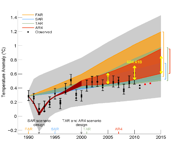
Figure 1. Second Order Draft Figure 1.4. Yellow arrows show digitization of cited Figure 10.26 of AR4.
Now here is the replacement graphic in the Approved Draft: this time, observed values are no longer outside the projection envelopes from the earlier reports. IPCC described it as follows:
Even though the projections from the models were never intended to be predictions over such a short time scale, the observations through 2012 generally fall within the projections made in all past assessments.
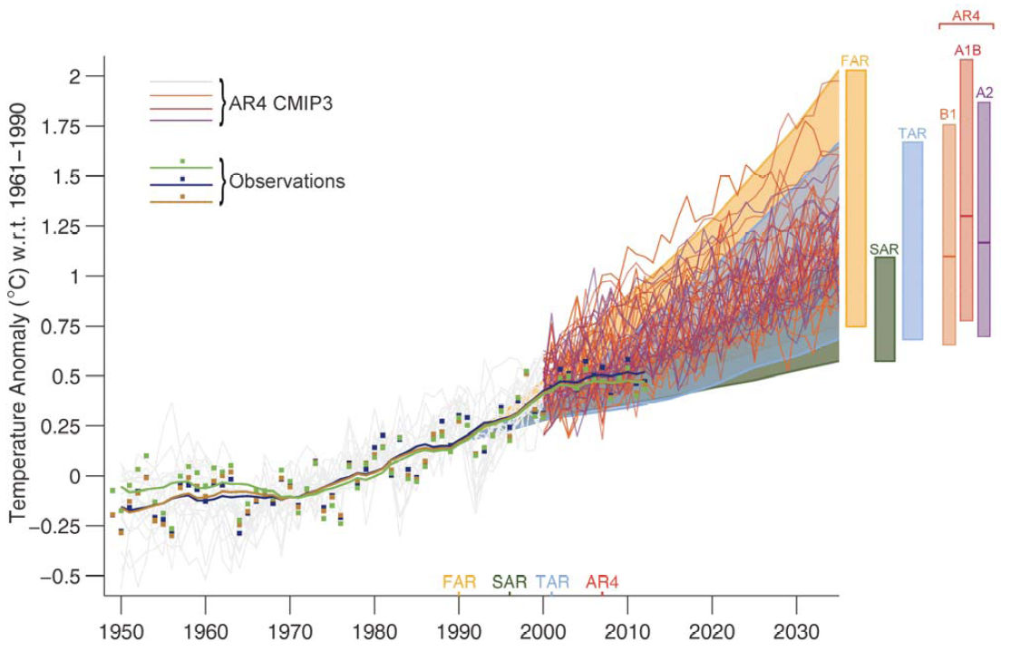
Figure 2. Approved Version Figure 1.4
So how’d the observations move from outside the envelope to insider the envelope? It will take a little time to reconstruct the movements of the pea.
In the next figure, I’ve shown a blow-up of the new Figure 1.4 to a comparable timescale (1990-2015) as the Second Draft version. The scale of the Second Draft showed the discrepancy between models and observations much more clearly. I do not believe that IPCC’s decision to use a more obscure scale was accidental.
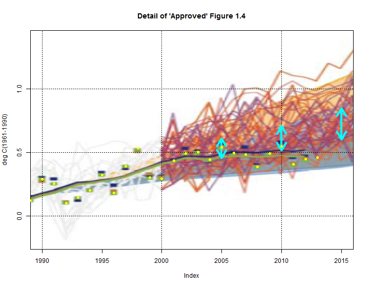
Figure 3. Detail of Figure 1.4 with annotation. Yellow dots- HadCRUT4 annual (including YTD 2013.)
First and most obviously, the envelope of AR4 projections is completely different in the new graphic. The Second Draft had described the source of the envelopes as follows:
The coloured shading shows the projected range of global annual mean near surface temperature change from 1990 to 2015 for models used in FAR (Scenario D and business-as-usual), SAR (IS92c/1.5 and IS92e/4.5), TAR (full range of TAR Figure 9.13(b) based on the GFDL_R15_a and DOE PCM parameter settings), and AR4 (A1B and A1T). ,,,
The [AR4] data used was obtained from Figure 10.26 in Chapter 10 of AR4 (provided by Malte Meinshausen). Annual means are used. The upper bound is given by the A1T scenario, the lower bound by the A1B scenario.
The envelope in the Second Draft figure can indeed be derived from AR4 Figure 10.26. In the next figure, I’ve shown the original panel of Figure 10.26 with observations overplotted, clearly showing the discrepancy. I’ve also shown the 2005, 2010 and 2015 envelope with red arrows (which I’ve transposed to other diagrams for reference). That observations fall outside the projection envelope of the AR4 figure is obvious.

Figure 4. AR4 Figure 10.26
The new IPCC graphic no longer cites an AR4 figure. Instead of the envelope presented in AR4, they now show a spaghetti graph of CMIP3 runs, of which they state:
For the AR4 results are presented as single model runs of the CMIP3 ensemble for the historical period from 1950 to 2000 (light grey lines) and for three scenarios (A2, A1B and B1) from 2001 to 2035. The bars at the right hand side of the graph show the full range given for 2035 for each assessment report. For the three SRES scenarios the bars show the CMIP3 ensemble mean and the likely range given by -40% to +60% of the mean as assessed in Meehl et al. (2007). The publication years of the assessment reports are shown. See Appendix 1. A for details on the data and calculations used to create this figure…
The temperature projections of the AR4 are presented for three SRES scenarios: B1, A1B and A2.
Annual mean anomalies relative to 1961–1990 of the individual CMIP3 ensemble simulations (as used in
AR4 SPM Figure SPM5) are shown. One outlier has been eliminated based on the advice of the model developers because of the model drift that leads to an unrealistic temperature evolution. As assessed by Meehl et al. (2007), the likely-range for the temperature change is given by the ensemble mean temperature
change +60% and –40% of the ensemble mean temperature change. Note that in the AR4 the uncertainty range was explicitly estimated for the end of the 21st century results. Here, it is shown for 2035. The time dependence of this range has been assessed in Knutti et al. (2008). The relative uncertainty is approximately constant over time in all estimates from different sources, except for the very early decades when natural
variability is being considered (see Figure 3 in Knutti et al., 2008).
For the envelopes from the first three assessments, although they cite the same sources as the predecessor Second Draft Figure 1.4, the earlier projections have been shifted downwards relative to observations, so that the observations are now within the earlier projection envelopes. You can see this relatively clearly with the Second Assessment Report envelope: compare the two versions. At present, I have no idea how they purport to justify this.
None of this portion of the IPCC assessment is drawn from peer-reviewed material. Nor is it consistent with the documents sent to external reviewers.


249 Comments
No need for peer-reviewing!
Just make the models colder!
But there is trouble brewing:
Their acts are trending bolder
They hoped you’d find this slower
Your research here is nifty
Their morals have slid lower
And like their lines, are shifty
===|==============/ Keith DeHavelle
Thanks Steve for exposing another logical fallacy:
Moving the Goalposts (Shifting sands; raising the bar; running for cover)
Humbug!: The Skeptic’s Field Guide to Spotting Fallacies in Thinking, Theo Clark, 2005 p101
“The goalie finally scores . . .and moves the goalposts. Goalie “Yes! I scored! . . .Granted, its an own goal, but as far as I’m concerned, a goal is a goal.”
On page 1-34 in the AR5-WG1 Final Draft, the report states how they modified the plot in Figure 1.4:
“For FAR, SAR and TAR, the projections have been harmonized to match the average of the three smoothed observational datasets at 1990.”
They simply moved the projections to match observational data at 1990 and get a better fit. It is basically an arbitrary change with, as you say, no justification. Amazing.
Steve: It looks like something else to me. In the Second Draft, they stated “Values are aligned to match the average observed value at 1990” – which sounds like a similar operation. This doesn’t explain why the placement in different in the final version.
How Inconvenient.
Very crafty! By continually do this they can hope that their faulty graphs will always appear as an upwardly acceleration of temperature shortly about to occr. This way they can never be proved wrong and their cash flow will remain intact as the catastrophe will always be but a few years into the future.
You’re seldom wrong when you back date your forecasts.
I think it is because they have renormalized all the prediction curves down so that they now sit on their wiggly smoothed data trend. The normalization point of 1990 is now sat nicely on one of the down wiggles of their fit instead of sitting on the actual measured anomaly for 1990. As a result all the predictions have conveniently shifted downwards by at least 0.15C. This then allows all TAR predictions to nicely envelope the data. Phew !
I guess this renormalization process could continue ad infinitum into the future !
No one renormalized anythink. Figure 1. isn’t from IPCC. Daily Mail tabloid newspaper created this, and claimed that its IPCC’s prediction, but that was a fake.
Figure 1 is from the IPCC’s Technical Summary of the first order draft for AR5, page TS-79:
Click to access TechnicalSummary_WG1AR5-TS_FOD_All_Final.pdf
The full draft is here:
http://www.stopgreensuicide.com/
Astounding. The ‘explanation’ is clear, but only in its intention to confound and blur.
This should be publicised. Cannot be dismissed as ‘whoops, just one mistake in a very big report’ ( like Himalaya 2035).
I was looking for some sign of humor in the IPCC text, like ‘fooled you with the first diagram’.
But they are playing for the tragic end…
That kind of action can only be explained by Groupthink, no sane mind would do this and not want to sink into the ground ashamed by the unexplainable embarrassment.
Some named person, or persons, created that graph.
It’s HIDE THE DECLINE all over again.
Crafty switch in presentation on their part. They must have taken a lot of heat for the original version, which had been all over the blogosphere as showing the data outside the range of the models.
By switching from “Values are aligned to match the average observed value at 1990″ to using “Annual mean anomalies relative to 1961–1990 of the individual CMIP3 ensemble simulations” they’ve simply widened the spread of the models to encompass the actual data.
Or another way to look at it, if we assume the focal point of the base year period is it’s midpoint (about 1975/76), they’ve shifted the focal point back 14/15 years.
“They must have taken a lot of heat for the original version, which had been all over the blogosphere as showing the data outside the range of the models.”
We’re very lucky those earlier drafts were leaked–the impact of their casting a light on the IPCC’s shiftiness could be profound, maybe eventually rivaling climategate, especially if the IPCC releases (or someone leaks) a document showing reviewers’ comments and author’s gatekeeping responses, and if someone who attended the SPM session leaks a few tidbits.
The comment by rogerknights in his post above is part of my take away from these revelations:
(1) The earlier suggestions at these blogs about revealing to the public at all stages of the IPCC AR5 process are validated. Those revelations allow the interested, and I would hope informed, observer to see how the process “works”.
(2) In this case we can readily see another of many examples that the IPCC process is biased towards spinning the evidence toward immediate government action on AGW.
(3) The time has probably come where blogs and other interested groups take the information reviewed and presented by the IPCC and provide their own conclusions and completely ignore those reported by the IPCC.
this is a brilliant suggestion
Which I labelled as shape-shifting, irony intended
The IPCC should hold a masterclass in “How to draw a complex-looking graph so as to reveal absolutely nothing”. It looks like somebody gave a 3-year-old graph paper and a box of crayons. Astounding.
As an engineer, when I present a graph, the intention is to give as much information as possible to the reader without ambiguity and without excessive clutter. This is the antithesis.
That’s the first thing I too thought looking at that graph. ‘someone is trying to not communicate something here’
I laughed. For all the world, it looks like the spiteful scribblings out of a child who couldn’t get his original effort to go as willed! It kinda says “Bah, who need science anyway?” Iconic.
I admit I wasn’t laughing as I waded into the adjusted spaghetti rather late. But the ‘Iconic’ got me. Thanks.
I’d take away his Crayolas and ban his foolscap drawing from my refrigerator door.
It gives a new meaning to ‘red noise’ in the climate context.
I have no idea what “harmonized” means in this context. Is this a real thing, and if so, could someone define it for the slower students?
Regardless of what this actually means, it appears obvious that if you change your projections so that they wrap around the means of the observations, then the observations will be somewhere in the middle of the projections. But all this means is that the original projections were plotted wrong somehow, if for no other reason than that they needed harmonization to match observations… that hadn’t yet occurred?
How do I go about becoming a climate scientist? It appears to be an ideal job, requiring perhaps only some serious study of Lewis Carroll. And maybe a hookah.
Btw, Keith, huge admirer of your poetry. 🙂
Hmm. I should’ve read further. My above comment doesn’t explain the difference from the current version of Figure 1.4 in AR5 and Figure 10.26 from AR4.
This is a masterclass in the art of beclouding,
pesadia,
Did you mean beclowning?
They are just buying themselves more time to further their politicised objectives. But the end is inevitable. If the media continues to ignore this failure of the models and malfeasance by the IPCC, non climate scientists need to speak up, else they will also suffer when the backlash comes.
Imagine if whoever drafted SOD figure 1.4 had chosen to align all the climate model output to 1989. Would you still be calling the figure “damning (but accurate)” or berating the drafter for cherry-picking a cold year for the alignment?
It should be rather obvious why aligning the model output to a single year is not sensible, so why the outrage when the IPCC ditches a poorly thought through figure?
Others will comment on the technical changes, but surely one issue with the new graph is that it was not shown to the external reviewers?
How many rounds of peer-review would you have the IPCC do?
If you will not accept any changes to the report that are not peer-reviewed, then after every edit the manuscript has to be sent back to the reviewers, who will doubtless suggest further changes, requiring more edits and yet another round of review. An infinite loop. This is plainly crazy, and is not how peer-review works in journals.
The data behind the SOD figure 1.4 and the final figure 1.4 are the same. The new figure is simply a different way of visualising the data.
Aren’t you confusing peer-review and IPCC review processes? IPCC AR is supposed to rely solely on peer-reviewed literature (what, as claimed, is not the case with this graph) and all that is written in the AR is supposed to be subject to external review process by reviewers (that as well, as claimed, has not been the case with this graph).
The claim by Steve:
“None of this portion of the IPCC assessment is drawn from peer-reviewed material. Nor is it consistent with the documents sent to external reviewers.”
Richard, this is EXACTLY how peer review works in journals. Every time you change a manuscript it has to go back to the reviewers. Once it’s been accepted you cannot change anything (except fixing minor typos). If you do propose a major change to a figure that alters a finding on a topic of central importance to your paper, it absolutely has to go out to the reviewers. Your excuse here is nonsense.
If the IPCC wants to use a system in which, time after time, key material is only inserted (or removed) after the close of peer review, then it should stop bragging about its peer review process. If it wants to boast of a rigorous peer review process then it should adopt one. After all, it was the IPCC’s self-proclaimed rigor of its peer review process that US courts and the EPA relied on when accepting IPCC findings for policymaking purpose.
Maybe your manuscripts need to be checked by the reviewers after ever change, but in general typically a manuscript is only sent for re-review if major revisions were required.
I suppose that you would like the IPCC to do an infinite number of rounds of peer review. Nicely tying up active scientists while you write your joke NIPCC report.
richard telford:
So you’re arguing that it’s okay to completely modify figures and not let the other authors see them before publication. That’s an amazing argument.
Of course the other authors would see the new figures before publication. What made you think otherwise?
Ross McKitrick:
Not quite true. Changes in a manuscript in response to a peer reviewer do not require re-review.
This is a different thing. It’s a substantively new figure. I would doubt an editor would allow it to appear in a journal without re-review. Given the collaborative nature of the reviews of AR5, not allowing the other authors to review is a breach of trust and ethics, in my opinion.
I should have said “do not *necessarily* require”. Whether a new peer review is needed depends on how substantive the changes are, and of course the editors make the final call on that.
richard telford:
Are you factually stating that all other authors of this chapter had the opportunity to review this figure?
And by “all” I mean “every other author” not just the inner circle.
Richard, I have explained in detail how I think the IPCC should structure its review process in my GWPF report here: http://www.rossmckitrick.com/uploads/4/8/0/8/4808045/mckitrick-ipcc_reforms.pdf
It wouldn’t involve tying up the IPCC authors in an infinite number of revisions. But it would block the IPCC Authors from continuing to claim that the final report has been peer reviewed even when conclusions depend on material inserted (or deleted) after the close of the review process.
“How many rounds of peer-review would you have the IPCC do?”
well
As many as O Donnell’s paper on the antarctic, or maybe as many as our paper which merely confirmed what the reviewers themselves had published.
In short.
The final draft should get a review.
“The data behind the SOD figure 1.4 and the final figure 1.4 are the same. The new figure is simply a different way of visualising the data.”
That’s testable Richard. do you have the data.. the data the actually used or will folks have to digitize shit.
Somebody made the charts. they have the data.
Steve: For the SAR envelope, I am convinced that IPCC applied the Tamino bodge. As others have observed, while Tamino’s centering method may well make more sense than choosing 1990 as a reference date, AR2 authors said that they used 1990 as a reference point. There’s a bigger problem lurking here, as Tamino misdescribed the purpose of the AR2 diagram and IPCC seems to have too quickly adopted Tamino’s misreading – without external peer review. On the AR4 envelope, Richard Telford’s assertion is not accurate: the Second Draft envelope was taken from AR4 Figure 10.26, while the Government Draft envelope is an interpretation of what they think AR4 ought to have done.
CMIP5 models are available to download and process. Tedious, though not too difficult, but you need a lot of disk space. Hopefully the data shown in each figure will be released as I suggested after AR4.
Richard
“CMIP5 models are available to download and process. Tedious, though not too difficult, but you need a lot of disk space. Hopefully the data shown in each figure will be released as I suggested after AR4.”
Well you have a problem there, since I have tried to download the data.
1. Do you know what models and what runs they used for each chart.
2. are you aware of the changes that have been made over time
3. Did they sample the GCMs in a masked fashion, ie only where hadcru had gridcells.
4. How did they transform the gaussian grids?
5. Did they plot the data correctly.
It would be easy to supply the actual time series used to create the chart.
That would facilitate checking.
Now of course you could have said.. “well get a computer an re run the models”
Bottomline, if you want folks to believe the charts, supply the data.
Im under no rational obligation to believe pixels on a page.
You are under no obligation to believe anything (except pixies). While supplying the data plotted in the graph would be useful, I don’t think it would materially affect your inclination to believe the figure.
If you want to audit the calculation of area-weighted mean temperature from the model output, go ahead. But you must be desperate to think you would find a fatal flaw in AR5 there.
Richard Telford, I’m having trouble believing what I’m hearing you say. So far, you have said, 1) there’s nothing wrong with them publishing this without re-submitting it for peer review. 2) there’s no reason why they have to supply the data (or the code) that they used to construct this, and 3) it’s unreasonable to be complaining about this or doubting their word.
Am I understanding you correctly? They should be able to post whatever graph they want, without any information on why it is right or how to check it, and all right-thinking people are supposed to just accept it?
1) The change to the figure was likely made in response to reviewer comments and been approved by the review editor. Unless you have an enormous number of review rounds some changes after the reviewers last saw the manuscript are inevitable. The change is minor and obvious. Has anyone any material objections to the new figure, which is using the same data, or is it all faux outrage?
2) The data are available to download and anyone familiar with model output would easily be able to process them to replicate this figure.
3) Complain all you like. It’s a tempest in a tumble that is diverting me from the critical review of the report I’m supposed to be writing.
Alright, I guess I believe it, since you’ve repeated it clearly. But I find it repulsive. Your words are taken directly out of the playbook of the Climategate Team: Don’t tell people how to get the result. Make sure that it’s obscure, by not providing data nor methods. Scoff at them for incompetence when they struggle to reconstruct something that should have been provided as a matter of course, and tell people that it proves that We are the professionals and Those Amateurs obviously don’t have a clue (see Dana’s lovely phrasing). If it turns out that the work is really mistaken or badly done, then say, What is all this faux outrage about that figure, anyhow – we’ve moved on and produced lots of newer better work which anyway gives essentially the same result.
Sorry, no. It’s not faux outrage. This is the kind of stuff that has convinced a decent and growing chunk of the world’s population that climate scientists aren’t scientists. If you care about climate science, instead of trying to cover for them, you should be tarring and feathering them.
Oh, sorry, I forgot: Never admit anything, no matter how obvious. You’re just giving ammunition to the enemy.
RE: Posted Oct 1, 2013 at 8:28 AM | Permalink | Reply
“The new figure is simply a different way of visualising the data.”
And in your view it’s not only a different way but a better way?
Since the draft figure is obviously flawed, of course the new figure, which avoids that flaw, is better.
If the draft figure is obviously flawed – as you tell us – I don’t understand figure TS.14 in the technical summary (p. TS-107).
Can you explain why the observations in the upper graph(s) are going to leave the predicted area of the models?
This graph supports fig. 1.4 of the second order draft.
And I don’t understand why the model graphs should be shifted “downwards” – maybe fitting to a reference year like 1992.
In 1992 the “global” temperature was reduced due to the outbreak of Pinatubo and is, therefore, no suitable reference year.
Furthermore, I don’t understand the discussion about a suitable reference year.
If the models used by the IPCC are a good representation of the observed “global” temperature they should perform a good hindcasting.
Fig 1.4 of the final draft starts at ~1950. So – why don’t the model graphs start at 1950, too?
Starting the model graphs at 2000 means to me that their hincasting skills may be miserable.
Richard claims that “The change is minor and obvious. Has anyone any material objections to the new figure, which is using the same data, or is it all faux outrage?” Whether it is material or not, is unknown.
As wernerkohl points out the shift makes backcasting an issue. The ability of models to backcast adequately to mimic the past was stated in Ch 9 AR4 as one condition necessary to attribute modern warming to anthropogenic influence. The reason given in Ch 9 was that the temperature reconstructions and models are not truly independent.
Another material objection was the use of unmeasured aerosol to help explain the cooler temperatures around 1940. This material objection not only has worsened due to the shift, it has been determined since AR4 that the aersol parameter used was too negative, thus indicating that this period should run even hotter. The lack of agrrement of backcasting and the temperature record is not immaterial to attribution.
Richard, the proper assumption at this time would be that the changes are material and that to support the changes, documentation is needed. Otherwise the claim of the same confidence could not be supported, much less an increase in confidence.
Also note that it is proper than when you redo something, you don’t just redo it to make it look like you wish, you redo it to a standard. If they are doing it to make the models look better for forecasting and it worsens the backcasting, it IS material and if true, it is a failure. The explanations, graphs and reasoning should be removed or changed to be correct. Otherwise the claim of it being the best science at present is falsified.
Yes Richard, but this was a major revision.
The bub of SMc’s comment is the statement
=========================
None of this portion of the IPCC assessment is drawn from peer-reviewed material. Nor is it consistent with the documents sent to external reviewers.
=========================
Richard Telford’s comment does not address this issue. If, as SMC notes, the new AR5 figure has no basis in peer-reviewed material and if it was not vetted by the reviewers then why was it published? Does SMc misapprehend the figure?
On a recent thread, I asked for a reference to help determine the relative offsets. Richard Telford claims there is an obvious reason why the whole endeavor is a bad idea; implying that each model should be aligned separately against … what?
The obvious thing to do is to make the offsets relative to the 1961-1990 climate normal period, or some other period if more appropriate. Picking a single year will end in tears.
Aren’t GCMs basically systems with initial value boundary conditions set? If so, then the question is “what did the model use as a baseline?” If it used the data in 1990, then that’s what it should be referenced against. If it used the average from 1960-1990, then that’s what it should be referenced against.
If it used the 1990 data as it’s starting point, then you can’t go back and plot it against the 1960-1990 average just to shift the plot. You’d have to go back and re-run the model at the new condition.
Richard Telford at Oct 1, 2013 at 4:33 AM:
“It should be rather obvious why aligning the model output to a single year is not sensible, so why the outrage when the IPCC ditches a poorly thought through figure?”
To complete a thought:
It should be rather obvious why aligning the model output to a single year is not sensible, so why the outrage when the IPCC ditches a poorly thought through figure [and replaces it with the Flying Spaghetti Monster]?
And replaces it with an even more poorly thought-through Figure, one which doesn’t honour earlier data
So, no problem then
What are you on about?
That’s my question
The earlier data I refer to are the model outputs from the 1960 period (your preferred baseline)
If one shape-shifts the baseline to honour earlier model output, these earlier outputs fail the error bars post 1998. If the shape-shift is moved to 1990 to honour later model outputs, the earlier outputs fail the error bars
So, no problem then
Shape-shifting? I don’t know any shape-shifters. And your figure does not illustrate your argument.
RIchard Telford: It is clear from AR4 Figure 10.26 (Steve’s Figure 4), that the A1B models predicted a slightly accelerating warming of 0.2 degC/decade over 2000-2020 period – a rate of warming which is very similar to that observed during the 1980-2000 period. You (and apparently the authors of AR5) are arguing that the y-intercept used in this fIgure from AR4 was inappropriate:
1) If the authors of AR5 believed that the authors of AR4 made a mistake, they should have clearly explained the earlier mistake. They should have added observations to AR4 Figure 10.26 and side-by-side shown what they now believe is a more-appropriate graph. By not openly and honestly confronting the contradiction between AR4 projections and subsequent observations, the authors of AR5 have created confusion for policymakers and the public. Skeptics can legitimately claim that the AR4 projections were wrong and others can claim that they were correct.
2) You may be correct in asserting that the 1990 start year was unusually warm, but it is also possible that it simply LOOKS warm because it occurred between two periods of volcanic cooling. Uncertainties associated with transient volcanic aerosols and decreasing anthropogenic aerosols confound the 1961-1990 baseline period for models.
3) The real issue is the SLOPE (rate of warming), not the y-intercept! You know (or should know) that few, if any, of the model runs in the “spaghetti” graph contain a 15-year period with negligible warming. As you also (should) know, Fyre (2013) found that it is “extremely likely” (p<0.05) that the warming of the past 20 years has been overestimated by models. So why are you and the IPCC attempting to obscure this simple fact with spaghetti graphs with adjusted y-intercepts? It's indefensible!
4) Suppose you were the editor of a journal that had received a paper discussing observations vs the authors earlier model projections. In their first submission (AR5 FOD), the authors include a graph that mis-located their projections from their previous paper (AR4 Figure 10.26), presumably by using the wrong reference period for calculating anomalies. As discussed in Steve's previous post, this mistake was detected by a reviewer. The authors revised their graph and also add an addition region of uncertainty that wasn't present in their earlier publication. During a second round of peer review, a reviewer notes that the revised graph shows that observations are now inconsistent with projections, contradicting the paper's conclusion. The authors revise their paper again, changing their projections for a third time (since they were originally published in AR4). They replace easily-understood confidence intervals with the "spaghetti" output from individual model runs AND add runs from additional emissions scenarios. Wouldn't you insist that the paper contain a full explanation of these changes and send that explanation out for another round of peer-review? Or would you simply reject such subterfuge?
+1
don’t expect an answer from Dr Telford anytime soon…until he consults the politburo
Frank,
Yours is the best summary I’ve seen of Dr. Telford’s defective reasoning. Point 1)is particularly telling. The essence of a scientific advance is being able to make significant theoretical predictions that are confirmed by experiment. If predictions fail the test of observation, that is a centrally important, if not fatal, matter.
You don’t get to simply go back and fudge your error envelope retrospectively to get agreement. Certainly if you do that sort of adjustment you had damn well better have some good reasons for it. You are clearly obliged to answer the question: If the convenient, newly adjusted error bars are the correct ones, why didn’t you use those back when you first made the prediction?
Under the circumstances is it just nitpicking, or unduly suspicious, to point out that the set of observations which runs colder in the last decade or so has been shown in a relatively pale shade of green?
First graph shows current observed temps at the 0.4 anomaly. Second graph at the 0.5 anomaly. 0.1 degrees of warming has been created out of nothing.
Reblogged this on Quixotes Last Stand.
According to environmental scientist Dana Nuccitelli, the “IPCC models have been accurate.”
Apparently climate contrarians are guilty of one for the following if they believe otherwise:
1) Publicizing the flawed draft IPCC model-data comparison figure
2) Ignoring the range of model simulations
3) Cherry Picking
See http://tinyurl.com/o4qn6do
Why push the outside of the envelope when you can push the entire envelope?
SkS says not to worry, IPCC model global warming projections have done much better than you think
http://skepticalscience.com/ipcc-model-gw-projections-done-better-than-you-think.html#.UkpVR8JIOhg.twitter
Steve, brilliant post by the way
I see they included the B2 emissions scenario, just to give a few more projections on the low side. In real life we’re right up there, see http://www.carbonbrief.org/blog/2011/06/iea-and-ipcc-temperature-projections
Stefan Rahmstorf from the PIK (http://www.pik-potsdam.de/) insists in his German blog that Figure 1.4 in the Second Order Draft contained an error:
http://www.scilogs.de/wblogs/blog/klimalounge/klimadaten/2013-09-27/der-neue-ipcc-klimabericht#comment-48839
He writes that the observed temperatures lie within the projected range of climate models. And he refers to Grant Foster who – according to Rahmstorf – had shown this error.
Could you comment this, please?
Thanks!
The SKS link Judy refers to above explains what Stefan is talking about. Apparently now the deal is picking which year you are aligning the values to. If it’s 1990, you get inside-the-projections values, if it’s a different year, you get outside-the-projections values. Each side accuses the other of cherry picking if you choose a year that shows a particular conclusion.
I personally think this notion of realignment is relatively new as it relates to the IPCC imagery. Everybody had all been going on the same maps for a while. Is Grant’s website cited for the changes when it comes to the new IPCC graphs? I wonder if he’ll be asking for such credit or if he’s just happy to help.
“The flaw is this: all the series (both projections and observations) are aligned at 1990. But observations include random year-to-year fluctuations, whereas the projections do not because the average of multiple models averages those out … the projections should be aligned to the value due to the existing trend in observations at 1990.”
From SkS site on Foster’s comment
Harmonise – don’t let observations charm your eyes
Let all those spaghetti graphs calm your eyes
.. and just harmonise, harmonise, harmonise
(only be sure to call it peer reviewed.)
(with apologies to Tom Lehrer)
Does AR5 have a millennium graph a la hockey stick? I can’t find it.
Seems that AR4 Figure SPM.5 would be even more telling, particularly in light of actual CO2 emissions:


First, our Skeptical Science friends showed that CO2 is following an almost worst-case scenario:
Then here’s AR4’s prediction of the warming that results:
Figure SPM.5. Solid lines are multi-model global averages of surface warming (relative to 1980–1999) for the scenarios A2, A1B and B1, shown as continuations of the 20th century simulations. Shading denotes the ±1 standard deviation range of individual model annual averages. The orange line is for the experiment where concentrations were held constant at year 2000 values. The grey bars at right indicate the best estimate (solid line within each bar) and the likely range assessed for the six SRES marker scenarios. The assessment of the best estimate and likely ranges in the grey bars includes the AOGCMs in the left part of the figure, as well as results from a hierarchy of independent models and observational constraints. {Figures 10.4 and 10.29}
Sure looks to me like the actual warming is following the orange “constant 2000 concentration” level. Hmmm.
I’m glad I’m not the only one who noticed this bait and switch game: actual CO2 has followed the “worst case” scenario, but actual warming has followed the “no additional CO2 at all” prediction. The models were falsified years ago if that is taken into account.
No matter how much you push the envelope, it is still stationary [sic, intentionally].
I think DGH’s link to Skeptical Science gives the explanation of what they did;
See http://tinyurl.com/o4qn6do
Also reprinted in The Guardian.
The key words are here:
“The first version of the graph had some flaws, including a significant one immediately noted by statistician and climate blogger Tamino:
“The flaw is this: all the series (both projections and observations) are aligned at 1990. But observations include random year-to-year fluctuations, whereas the projections do not because the average of multiple models averages those out … the projections should be aligned to the value due to the existing trend in observations at 1990.
Aligning the projections with a single extra-hot year makes the projections seem too hot, so observations are too cool by comparison.”
Thus, instead of starting the projections at the 1990 temperature value (around 0.3), they started them at an ‘average’ temperature for that period (eg. a five-year mean centred on 1990, approx 0.2). This brings all the projections down by about 0.1 degC. Removing the error bars also helps. This does not seem enough on its own, but is at least a big part of the adjustment.
What I found telling about Dana’s post is the fact that his excuse for the original error was that it was contained in an early draft. Ooops. On the other hand he argues that this plot – which has just now become public and has not been peer reviewed – is correct and forms the basis of the statement, “IPCC models have been accurate.”
Indeed we’re supposed to believe that the IPCC should be excused for an error and simultaneously believe that the organization is infallible.
Regarding your Figure 4, it’s even worse than that. Seeing that HadCRUt3 contains an artificial step change of about 0.064C (based on the fact that HadSST2 shifted up suddenly and permanently by ~0.09C relative to all other global SST datasets across the transition from 1997 to 1998, when Hadley Centre switched data sources for their product) that has never been addressed, much less amended (rather covered up when presenting their new and ‘improved’ HadCRUt4), the actual HadCRUt3 graph should compare rather like this with HadCRUt4 shown here:
http://woodfortrees.org/plot/hadcrut3gl/from:1978/to:1998/compress:12/plot/hadcrut3gl/from:1998/offset:-0.064/compress:12/plot/hadcrut4gl/from:1978/offset:-0.01/compress:12
Playing with the starting value only determines whether the models and observations will appear to agree best in the early, middle or late portion of the graph. It doesn’t affect the discrepancy of trends, which is the main issue here. The trend discrepancy was quite visible in the 2nd draft Figure 1.4. All they have succeeded in doing with the revised figure is obscuring it.
I prefer comparisons of trends like this.
I actually happen to think the AR4 is no better than the figure it was replaced by, and possibly worse because of the way the data series were aligned. My objection with both figures is in that you are plotting a projection from a scenario (rather than a forecast based on actual forcing data) on the same graph, as if you were comparing forecast outcome with actual outcome.
What would be an interesting comparison for me would be to show would happen if you ran e.g. the AR4 models further forward to 2013 (or as recent as is practicable) using the actual forcings, starting with the exact run states of the models at the stopping point of the last simulations.
A good reminder of the best visual.
One can only wonder what else will come to light as the underlying papers are published. Habitual mendacity is so reliable.
Pointman
BTW. Slight typo Steve – Klimazweiberl s/b Klimazwiebel.
The original graphic appeared in Judith Curry’s article in
‘The Australian Newspaper on the 21st of September’ so is
on the record. No down the memory hole with it.
Climate science takes the Fifth…. Assesment….
Good lord– in no other field of professional endeavor would such obviously manipulated discrepancies be accepted for a moment. Absence of peer review in sense of replicating findings is a serious omission, virtually admitting that doctored inputs have been illegitimately processed.
As years go by, such asininities are not sustainable. Any so-called researcher (“scientist” is the wrong word) or global “policy maker” [sic] claiming IPCC support is due for rude awakening.
I combined the two plots into an animated gif to be able to see the effect of the changes:
I don’t recall that in the previous assessments, the “correct” methodology of selecting the common starting point using trends. I am pleased to see that the proper adjustments have now been made to solve this previously unrecognized problem.
Thanks, very helpful.
AC
Why would they include AR4: A1B, A2 and B2 for the points in time where we have data against the actual predictions for the actual scenario (we’ve been roughly following A2).
Wouldn’t it be clearer to just include AR4[A2] for the period of time that we already have measurements for, then plot their best predictions moving forward with various scenarios as clear bands as was in the draft copy?
The observations hidden within the spaghetti strands look to be only the high end of the ranges displayed before. Especially for the years following 2000 temperature data point placement is higher to apparently vindicate the model runs.
And still, even with the shaded areas (allegedly the 90% confidence predictions) replaced by a spaghetti-graf (with shifted shadings) ..
.. where the spaghetti-lines are unsmoothed to appear presenting a wider range than plotted actual and even filtered smoothed temperatures ..
.. still, the only thing those are showing is that occasionally one spaghetti-line will dip below observations for one point.
And with many spaghetti-lines you can at least create the impressions that there are a couple of points falling below even under observed temperatures. But mutually different lines, and each line’s trend is distinctly higher than observations.
Not even with this new trick to conceal the decline can they give any such impression other than optically and superficially!
I just saw that Lucia’s had a very convincing argument (to me at least) on Tamino’s (and IPCC’s) approach.
http://rankexploits.com/musings/2013/leaked-chapter-9-ar5-musings/#comment-119655
“lucia (Comment #119655)
September 24th, 2013 at 8:55 pm
I should add: Also, consistency with Tamino’s notion of picking the 1990 ‘point’ based on the trend line means that he should align the trendline through the models to the trendline for the observations. Instead, he aligns the value of the model mean at 1990 to the trendlinefor the observations. That’s applies and oranges.
(Moreover, if he aligns trendlines at 1990 for both models and observations, and fits the trend from Jan1980-Dec1990, he will actually match the projections from the AR4. Because that’s the way OLS works!”
She has a new post where she makes it still clearer

http://rankexploits.com/musings/2013/taminos-take-on-figure-1-5/
Her figure
is nothing short of hilarious.
I wonder if the von Storch paper is referenced in AR5?
“…we find that the continued warming stagnation over fifteen years, from 1998 -2012, is no longer consistent with model projections even at the 2% confidence level.” http://www.academia.edu/4210419/Can_climate_models_explain_the_recent_stagnation_in_global_warming
Oops, actually I think it was a little too late.
Please note: von Storch’s paper was written and published BEFORE the AR5 SOD was modified.
In the AR4 10.26 GLB Temperature graph, isn’t it funny how the AR4 model follows the temp time series up to a certain point, but then suddenly switches to a smooth upward slope? I’m no math guy, but it seems like they’re going from modeled output, and then tacking on a smoothed trend at the end. Isn’t this like comparing apples to antelopes?
Maybe I’m completely wrong. But going from noisy to smooth seems bogus.
The CMIP3 runs used historical forcings for the 20th century — so e.g. they show a response to Pinatubo and El Chichón — but for the 21st they used projected forcings. See here. The multi-model mean is generally smoother than observed temperatures because the “weather noise” gets averaged out, but for volcanic eruptions, the models will have a synchronized “bump” and the mean will be affected.
Another pea??
The AR5 (SOD) Chapter 1 states this about climate model performance: “In summary, the globally-averaged surface temperatures are well within the uncertainty range of all previous IPCC projections, and generally are in the middle of the scenario ranges.”
The AR5 Final replaced the above with: “In summary, the trend in globally-averaged surface temperatures falls within the range of the previous IPCC projections.”
The Pea has and eye to the left and two seas to the right…
More AR5 trend shifting shenanigans here:
Here’s what Dana is saying:
” … McIntyre doesn’t say anything of substance. His post is basically “I don’t understand why they shifted the data up.” Ever heard of proper baselining? Tamino figured this out 10 months ago. I guess that goes to show who’s the better statistician. If you don’t trust the figures or baselining, then look at the trends as I did. McIntyre doesn’t even take that first simple step to analyze the data. Totally worthless post.”
I’m just a layman. If there’s no substance in what Dana is saying maybe Steve would drop by and put him right – see http://www.theguardian.com/environment/climate-consensus-97-per-cent/2013/oct/01/ipcc-global-warming-projections-accurate?commentpage=1
TC
TC, see Sven’s comment above.
For all I know, Tamino might be absolutely right about how the IPCC should choose baselines for its forecasts going forward. But to me it’s self-evident that, when your forecast takes the form of a delta applied to some baseline, the baseline has to be specified at the time the forecast is made, and adhered to when testing the forecast against observations– even if you think ex post that a different baseline would have been better.
Paul,
You are exactly right of course. We see folks like Tamino and Richard Telford above arguing that the data should be presented properly, and after that is done, the projections fall in line with the observations. So far, so good. But from there these same folks want to take it further and claim that the IPCC projections have been validated. In doing so, they betray the fact that they have no idea how hypotheses are properly adjudicated via the scientific method. I shall attempt an analogy. The soccer player launches the penalty kick and it misses the goal to the right by one foot. Tamino sprints along the end line with his measuring tape and discovers that the goal was actually placed three feet closer to the left corner of the field than the right. Now that the discrepancy has been rectified, we are being told that the proper thing to do is credit the kicker with the goal.
TC
“I’m just a layman. If there’s no substance in what Dana is saying maybe Steve would drop by and put him right” – at The Guardian
No chance. Any uncomfortable comments are routinely censored.
Seems pretty obvious that the IPCC can’t, as an organization, ever openly acknowledge significant discrepancies between projected warming and reality, since that would simultaneously undermine the credibility of all their projections, and reduce the IPCC’s claimed urgency for rapid reductions in fossil fuel use. Since many government funded researchers from the USA were involved in the IPCC AR5 report, it would seem reasonable for a congressional committee to call some of them to testify and explain the kinds of shenanigans Steve lays out in this post. I find the audacity in this kind of deceptive presentation both offensive and almost unbelievable. Could any of them really think this is ‘OK’?
Ok so if adjusting the data upwards doesn’t work well enough we’ll adjust the projection envelopes downwards.
That will fix our salaries for the next fifteen years.
Has anybody looked at how this changes the backcasting? IIRC, AR4 showed that the backcasting was reasonably fit.
That’s a good question. It looks to me like the actual temperatures are now running to hot from 1950-1970, by roughly the amount that they shifted the projections downwards by.
Carrick, have you read Ch 8 of AR5? I have started it. If I am reading it correctly, there is a claim that AR4 models would be running even hotter (if they matched the real system) due to the re-evaluation of aerosols and aerosol interactions. It is hard reading, but it appears to me that the sum of differences are being used to explain the divergence by what is needed to explain and not most likely. Have you had a chance to look at this?
With Ch 8, the bodge, and temperature data, changing one aspect opens the question of why only those that bring the projections and temperature closer, and not an even handed scientific approach.
If you add the shift of .1C to the backcasting, and redo the aerosol bodge for periods like the 1940’s while backcasting, I don’t think the AR4 models will look very good.
In other words, I believe the IPCC in trying to explain the pause have made their whole AR4 unbelievable. This is based on how the parts re-enforced each other. Now we have an explanation that severely compromises, IMO, that re-enforcement. Hopefully when the final comes out, it will be explained.
You don’t have to look at backcasting to find an inconsistency.
In the initial plot, the SAR scenario design is fitted to an initial lower temperature to accentuate the three years of subsequent temperature increases before the SAR was released. According to the recently invented paradigm, the starting point should be moved up to a “trend” value which would push the corresponding envelope about 0.2 degrees higher than it is in the later plot.
Otherwise it is more “apples and oranges”!
RomanM, I think that should be read more “apple to cherry pie”.
Lucia’s point of using this:””The report clearly states that the projections are relative to the mean of Jan1980-Dec1999 temperatures. That’s what it says. That’s what one should use.””
But IIRC, one of the reasons it did this was that otherwise the backcasting was not very good. Baselines seem to change when it is to “explain” away problems.
Steve: AR4’s reference in figure 10.26 was,as Lcuia says, 1980-1989 and obviously that’s what should be used. AR2 descrines the reference as 1990. Presumably they were aware that 1990 was warmer than 1992 and had the opportunity to take that into consideration.
Relax guys. It’s a dodgy trick, and they can only pull it once. Every time they move the goal posts, the Internet preserves the post holes.
Preserving the post holes only matters if you gather up the adjustments and present them in understandable ways, as well as ensure that all the adjustments are not applied selectively. That’s a lot of work and so far as I can tell it hasn’t been done.
If you are looking for a laugh, check out Figure TS.14. It show the ‘indicative likely range'(whatever that means) of global average temperature through 2035. The 2035 projection now covers everything from essentially flat temperatures for 20 years to warming at >0.25C per decade. The funny part is that the bottom of the ‘indicative likely range’ now falls completely outside the ENTIRE 299 run ensemble of CGM projections. So I guess even the IPCC authors understand that the GCM’s are projecting too much warming, they just can’t officially admit that the model projections are wrong. The best part of this graphic is that it guarantees the IPCC projections of warming can NEVER be proven wrong again, no matter how the next 20 years goes…. global warming catastrophe and urgent draconian reductions in fossil fuel use are now justified by… well, even the possibility of no warming. Politically prudent, but making the projections (and the report itself), useless in formulation of meaningful public policy. You just gotta love the “I’m right and you can never prove I am wrong” approach, which seems, sadly, a recurring theme in climate science.
TS.14 is talked about on page TS-48 (p51 in the pdf from here) and provided on TS-107 (p110). Like you I’m not sure what the pink ‘indicative likely range’ means but isn’t this graph meant to show the spread of GMST for all RCPs? Could that explain the low lower bound in 2035? Isn’t the problem from 2000 to the present that we’ve been emitting almost at the worst case level, as Mr Pete pointed out earlier?
But I’m very willing to be corrected. Brighter bulbs than me find the output of the IPCC less clear than it might be.
As Ross pointed out, the focus should be on the trends, not whether or not the observations are falling within the model variability envelope. The latter is a diversion.
Lucia is doing a lot of good work on the CMIP5 trends, and we have assembled the noise about the CMIP3 model mean trend in this work (that was unfortunately, never published). The key to assessing model performance is whether or not the observed trend fall within the modeled trend pdf.
-Chip
The green line diverge from others datasets before 1980 and after 2000.
erratum: before 1970
The current IPCC chart could/should be referred to as a Spaghetti Monster.
Ah, it seems to me that they’ve just used (a slightly modified versiof of) Tamino’s Trick (see the part of the rant starting “What about the plot from the draft of the AR5 report?”): all model values are pinned to 1990 (zero?) while observations are relative to the 61-90 baseline. In the draft version all values (including observations) were pinned to a value in 1990. Even if you accept Tamino’s justification (I do not) for this, it’s still wrong: models should be pinned to zero in 1975 (midpoint of the observation baseline) not something in 1990.
I guess the term of the day is “harmonization”, see the figure caption on page TS-96:
Steve: yes. for the SAR version, they definitely seem to have used Tamino’s Trick – or perhaps, in this context, the Tamino “bodge”. The amount that IPCC bodged the envelope is almost exactly in accordance with the Tamino bodge. I’ve looked back at the underlying SAR report and there’s another layer of the onion to peel.
Jean S,
Tamino strikes me as a somewhat disreputable source of information… always tilted towards catastrophe. I would not pay much attention to his pronouncements, IIWY.
Why is it so difficult to establish what the offsets should be? All the data is (groups of) anomalies against some (common OR NOT to the group) baseline. Whether that baseline is a year (1990) or a range of years (1960 – 1990) should all be well-defined by the data sets. Why are these questions even under debate?
does it really matter ? if they move the trend it affects the hindcasting,so the models are falsified by past observations ,if they dont,the models are falsified by recent observations .
so they are wrong no matter what year they pick for the start point ?
forget about the peer review process,it supports nothing about the actual content,only that other academics agree the methodology is reasonable.
@bit chilly
if they move the trend it affects the hindcasting,so the models are falsified by past observations
All true. But the chart “Hides the Hindcast” by reducing to minimum the color saturation of the calibration portion of each model.
The eye is drawn to the difficult to resolve 1990-2050 part of the chart. But the crime scene in in the 1970-1990 portion of the chart with impossible to resolve lines of the models. The decline in fit to data is hiding in plain sight.
Dissection of the goodness of fit of the models to the 1970-1990 interval before and after the shift applied to the Approved version should be enlightening.
[Please delete 11:45 am and this post. 11:52am is a better formatted replacement.]
@bit chilly
if they move the trend it affects the hindcasting,so the models are falsified by past observations
All true. But the chart “Hides the Hindcast” by reducing to minimum the color saturation of the calibration portion of each model.
It is nearly the same graphical trick as hiding the Briffa decline but applied in reverse. Instead of erasing the one inconvenient line, they reduce saturation to 95%, remove color, and widen the lines — 39 times.
The eye is drawn to the difficult to resolve 1990-2050 part of the chart. But the crime scene in in the 1970-1990 portion of the chart with impossible to resolve lines of the models. The decline in fit to data is hiding in plain sight. (climateaudit 12/1/2011)
Dissection of the goodness of fit of the models to the 1970-1990 interval before and after the shift applied to the Approved version should be enlightening.
Amazing analysis Mr. McIntyre. Well done!!
Another graph dealing with models projections is on page 120, Figure 11.25 of Chapter 11. The graph shows a different presentation on global mean temperature then contained in the Chapter 1 document which is the subject of this post. However it looks like the right hand did not know what the left hand was doing in that the Chapter 11 diagram shows the models far off the mark in projecting temperatures versus measured data.
Looks like they have modified the unexplained gray bands into some sort of spaghetti graph that can swallow the observations.
Using a spaghetti graph seems a crude trick to widen the prediction bounds by including not only the “natural variation” (or weather-like) year-to-year randomness from the GCM runs, but also the runs between completely unrelated models. The lowest-sensitivity models are not yet inconsistent with observations, so they’re claiming success. It would be impolite to point out that the observations barely are keeping contact with the runs from lowest-sensitivity models which also have the most negative weather excursions. As mentioned by John Davis above, the IPCC has also included B2 runs, which may well have provided the low-hanging linguine.
The IPCC has widened the prediction window to include the observations. If the “Texas sharpshooter fallacy” is to draw an unrealistically small circle about a bullet hole in a barn (and claim that’s where one was aiming), here the IPCC is saying “Well, I only said I’d hit the barn. Doesn’t matter where, does it?” [It would be cynical of me to suggest that if observations had matched the AR4 A1B multi-model mean fairly well, that the IPCC would claim that validates the use of the multi-model mean.]
In a like vein, it’s disingenuous to include the entire range of FAR predictions, from “business as usual” to scenario D — “stringent controls in industrialized countries combined with moderated growth of emissions in developing countries”. Scenario D has clearly not occurred. The IPCC should compare observations with the low/best/high estimates of “business as usual”, given in FAR SPM Figure 8. [All time series re-baselined to some common period such as 1961-1990.]
All these shenanigans just so they could say that “temps are consistent with the models” and hope that the public buys it (they know that we “flat Earthers” know it isn’t true). What utter tosh.
Do the few CMIP3 and CMIP5 model runs that do not run hotter than observations have values of atmospheric CO2 concentration that even closely approximate what actually occurred? In my opinion, only model runs that had CO2 at realistic (observed) levels should even be considered.
According to the new graph, there could be a cooling trend right through to 2035 and it would still match the models’ projections.
“We’re very lucky those earlier drafts were leaked”
Does any other science rely so crucially on leaks to make any progress?
Steve, as I’ve pointed out on a number of equations, there are much worse considerations in the graphs above. The spaghetti they present deliberately provides the illusion — as you and indeed they directly point out — that current temperatures lie within an “ensemble” of single model runs drawn from the collection of models presented.
Let us count the sins:
a) Let me choose the single model runs to put into the figure, and by running each model a few dozen times and picking the one run I include, I can make the figure look like anything at all. God invented Monte Carlo to help stupid, confirmation biased sinners avoid the deliberate or accidental abuse of statistics described by its own chapter in “How to Lie with Statistics”. To Hell with it.
b) We cannot be certain that they did, in fact, choose the model runs to include. Maybe they did just pick them “randomly”. In that case, their conclusion is a clear case of “data dredging”, only worse. This is a mortal sin even without cherrypicking.
When one does ordinary data dredging, one takes 20 jars of jelly beans, feeds them to lots of people, counts the number with acne, and discovers that green jelly beans can be positively correlated with (and hence “cause”) acne, because they beat the usual (but meaningless) cut-off of 0.05 where all of the others fail. Of course with 20 jars it is PROBABLE that one will make the cut-off, and with enough colors, one can beat even more stringent limits there are what, over thirty colors of GCM “jelly beans” in this ensemble?
If only this were the worst of it, it would be easy enough to fix. One has to use a more stringent distribution and statistical test when one has an ensemble of independent jars of jelly beans, but there are still levels of correlation between green jelly beans and acne that would be difficult to explain with the null hypothesis of no correlation.
But now take one of the actual jelly beans OUT of the jar above, that contains thirty different colors of jelly beans in a SINGLE jar. Yes, there are places where the green jelly beans are correlated with acne — some people that got acne did indeed eat green jelly beans. Most, however, did not. Some people that got acne ate more red jelly beans and no so many green. Most, however, did not. In fact, every single one of the jelly bean colors individually FAILS a simple hypothesis test of good correlation with acne — really even barely marginal correlation with acne — but nearly all colors of jelly bean had a few days (not the same days) where they were well correlated among many more days they were not.
The graph above is in the unique position of stating that while EVERY color of jelly bean INDEPENDENTLY fails a hypothesis test against the data, we can be certain that jelly beans cause acne because every color of jelly bean has at least a few people who ate that color and got acne.
This isn’t a small, ignorable error. This leads to a simple pair of possibilities. Either the assemblers of the graph and drawers of conclusions from the graph are completely incompetent at statistical hypothesis testing and data dredging and managed to put a poster child case of data dredging front and center in the report for policy makers, in which case they should be summarily fired for incompetence and replaced with competent statisticians, or else (worse) they are COMPETENT statisticians and deliberately assembled a misleading graph that openly encourages the ignorant to dredge the data by interpreting the fact that nearly every model dips for TINY INTERVALS OF TIME down to where they reach the measured GAST (but they all do it at different times, spending much less than 5% of their time down there) as evidence that collectively, the model spread includes reality. Oh, My, God. To Hell with you, sinner!
c) The next two sins are closely related. In AR4 and the early draft of AR5, the mean and standard deviation of the collection of models was presented (graphically, at least) as a physically meaningful quantity. I say standard deviation because without the usual normal/erf assumptions, how can they generate confidence levels AT ALL? The basis of nearly all such measures in hypothesis testing is the central limit theorem, especially lacking even a hint of knowledge of the underlying distribution.
However, this is in and of itself a horrible, mortal sin against the holy writ of statistics. The central limit theorem explicitly refers to drawing independent, identically distributed samples out of a fixed underlying distribution. There is no POSSIBLE sense in which the GCMs included in the graphs above are iid samples from a statistical distribution of physically correct GCMs. There IS NO SUCH THING (yet) as the latter — the GCMs don’t even MUTUALLY agree within a sensible hypothesis test — started with identical initial conditions in trivial toy problems they converge to entirely distinct answers, and if one does Monte Carlo with the starting conditions the (correctly formed) ensemble averages per GCM will often fail to overlap for different GCMs, certainly if you run enough samples.
The variations between GCMs are not random variations. They share a common structure, coordinatization, and in many cases similar physics similarly implemented. The mean of many runs of INDEPENDENT GCMS is not a statistically meaningful quantity in any sense defensible by the laws of statistics. The standard deviation of that mean is not a meaningful predictor of the actual climate. One can average HUNDREDS of failed models and get nothing but a very precise failed model, or “average” a single successful model and have a successful model. So to present such a figure in the first place is utterly misleading. To Hell with it.
c) The GCMs are not drawn from an iid of “correct GCMs”. Therefore their mean and standard deviation is already a meaningless quantity, no matter how it is presented. There is no basis in statistics for the quantitative evaluation of a confidence interval, lacking iid samples and any possibility of applying e.g. the central limit theorem. Evil Sin, to Hell with it.
I was afraid AR5 would persist in the statistical sins told in the summary for policy makers in AR4, and it appears that they have indeed done so, and even added to them.
To CORRECT their errors, though, is simple. Just draw each jelly bean (colored strand of spaghetti) against the data ALONE. For EACH model ask — is this a successful model? Not when it spends well over 95% of the time too warm. Repeat for the next one. Ooo, reject it too! Then the next one. Outta here!
In the end, you might end up with ONE OR TWO models from the entire collection that only spend >>80%<< of their time too warm, that aren't rejected by a one at a time hypothesis test per independent GCM. Those models are merely probably wrong, not almost certainly wrong.
Or, apply a Bonferroni analysis in order to obtain the p-value for the complete set. Oooo, does THAT fail the hypothesis test of "what is the probability of getting the actual data, given the null hypothesis that all of these models are in fact drawn from a hat of correct models". Since NONE of them are even CLOSE to the actual trajectory and one would expect at least one to BE close by mere chance given over 30 shots at it, be can reject the whole set (slightly fallaciously).
Finally, we could look at, I dunno, second moments — the FLUCTUATIONS of the models. Do they bear any resemblance to the actual fluctuation in the data? No they do not, not even as single model runs. Indeed, the single model runs could be rejected on this basis alone — why would the year to year variation of the climate be changing when it has historically been remarkable stable in the entire HADCRUT record, with the exception of a single decade that is almost certainly a spurious error back in the 19th century?
To Hell with it.
rgb
rgbatduke–
Well, for one, I appreciate your taking the time to write up this comment–for me, at least (a non-statistician), it does an excellent job of explaining the sins. Well, for two, posts/comments like this are a major reason that I read CA–I get to be educated about it all. Thanks to you here, I believe I come away with a much clearer understanding. “But I am in/So far in blood, that sin will pluck on sin.” –IPCC, aka “Richard III”
Thanks, Prof. Brown. Once again, you help to educate and inform us in language that non-scientists can understand.
Given that the choice of baselines is so critical in these exercises, my flabber is gasted at the way they did this. When I was involved in (quite different) research, one of the first things we did was to play around with different baselines as a reality check. Choosing your baseline is one of the most important decisions you make, and requires a lot of thought and testing.
In this excellent post, Dr. Brown (rgbatduke) has provided yet again a superb framework on which physicists and engineers who have at least a tentative sense of distrust in the proffering of AGW alarmists can organize their thoughts. In this instance, we may feel that the mainstream climate scientists are moving the “road signs” of doubtful models, and trying to justify an envelope of model outcomes based on the contention that an 18-wheeler once went through a guard rail here and into a cornfield – to say that the muddy ruts are really part of their model’s road. Dr. Brown has called out the statistical sins involved. And he has told us exactly what to look for:
“To CORRECT their errors, though, is simple. Just draw each jelly bean (colored strand of spaghetti) against the data ALONE. For EACH model ask — is this a successful model? Not when it spends well over 95% of the time too warm. Repeat for the next one. Ooo, reject it too! Then the next one. Outta here!”
This insight he has provided is of immense value. Thanks again Dr. Brown. Please give his post careful study.
Rgb, excellent summary. However, shouldn’t the first sentence use “occasions” instead of “equations”?
Funny you should ask:-) Yes, but the error is subtle enough to be a halfway decent pun.
As for elevating it to a full post (later comments) — if I were going to do an actual post on it, I’d only feel comfortable doing so if I had the actual data that went into 1.4, so I could extract the strands of spaghetti, one at a time. As it is, I can only see what a very few strands of colored noodles do, as they are literally interwoven to make it impossible to track specific models. For example, at the very top of the figure there is one line that actually spends all of its time at or ABOVE the upper limit of even the shaded line from the earlier leaked AR5 draft. It is currently a spectacular 0.7 to 0.8 C above the actual GAST anomaly. Why is this model still being taken seriously? As not only an outlier, but an egregiously incorrect outlier, it has no purpose but to create alarm as the upper boundary of model predicted warming, one that somebody unversed in hypothesis testing might be inclined to take seriously.
But then it is very difficult to untangle the lower threads. A blue line has an inexplicable peak in the mid-2000’s 0.6 C warmer than the observed temperatures, with all of the warming rocketing up in only a couple of years from something that appears much cooler. Not even the 1997-1998 ENSO or Pinatubo produce a variation like this anywhere in the visible climate record. This sort of sudden, extreme fluctuation appears common in many of the models — excursions 2 or three times the size of year to year fluctuations in the actual climate, even during times when the climate did, in fact, rapidly warm over a 1-2 year period.
This is one of the things that is quite striking even within the spaghetti. Look carefully and you can make out whole sawtooth bands of climate results where most of the GCMs in the ensemble are rocketing up around 0.4 to 0.5 C in 2-3 years, then dropping equally suddenly, then rocketing up again. This has to be compared to the actual annual variation in the real world climate, where a year to year variation of 0.1 or less is typical, 0.2 in a year is extreme, and where there are almost no instances of 3-4 year sequential increases.
I have to say that I think that the reason that they present EITHER spaghetti OR simple shaded regions against the measurements isn’t just to trick the public and ignorant “policy makers” into thinking that the GCMs embrace the real world data, it is to hide lots of problems, problems even with the humble GAST anomaly, problems so extreme that if they ever presented the GCM results one at a time against the real world data would cause even the most ardent climate zealot to think twice. Even in the greyshaded, unheralded past (before 1990) the climates have an excursion and autocorrelation that is completely wrong, an easy factor of two too large, and this is in the fit region.
Autocorrelation matters! In fact, it is the ONLY way we can look at external macroscopic quantities like the GAST anomaly and try to assess whether or not the internal dynamics of the model is working. It is the decay rate of fluctuations produced by either internal feedbacks or “sudden” change in external forcings. In the crudest of terms, many of the models above exhibit:
* Too much positive feedback (they shoot up too fast).
* Too much negative feedback (they fall down too fast).
* Too much sensitivity to perturbations (presuming that they aren’t whacking the system with ENSO-scale perturbations every other year, small perturbations within the model are growing even faster and with greater impact than the 1997-1998 ENSO, which involved a huge bolus of heat rising up in the pacific).
* Too much gain (they go up more on the upswings than the go down on the downswings, which means that the effects of overlarge positive and negative oscillations biases the trend in the positive direction.
That’s all I can make out in the mass of strands, but I’m sure that more problems would emerge if one examined individual models without the distraction of the others.
Precisely the same points, by the way, could be made of and were apparent in the spaghetti produced by individual GCMS for lower troposphere temperatures as presented by Roy Spencer before congress a few months ago. There the problem was dismissed by warming enthusiasts as being irrelevant, because it only looked at a single aspect of the climate and they could claim “but the GASTA predictions, they’re OK”. But the GASTA predictions above are the big deal, the big kahuna, global warming incarnate. And they’re not OK, they are just as bad as the LTT and everybody knows it.
That’s the sad part. As Steve pointed out, they acknowledged the problem in the leaked release, we spent another year or two STILL without warming, with the disparity WIDENING, and their only response is to pull the acknowledgement, sound the alarm, and obfuscate the manifold failures of the GCMs by presenting them in an illegible graphic that preserve a pure statistical illusion of marginal adequacy.
Most of the individual GCMs, however, are clearly NOT adequate. They are well over 0.5 C too warm. They have the wrong range of fluctuation. They have absurd time constants for growth from perturbations. They have absurd time constants for decay from perturbations. They aren’t even approximately independent — one can see bands of similar fluctuations, slightly offset in time, for supposedly distinct models (all of them too warm, all of them too extreme and too fast).
Any trained eye can see these problems. The real world data has a completely different CHARACTER, and if anything, the problems WORSEN in the future. I cannot imagine that the entire climate community is not perfectly well aware of the “travesty” referred to in Climategate, that the models are failing and nobody knows why.
Why is honesty so difficult in this field? As Steve Mosher pointed out, none of this should ever have been used to push energy policy or CAGW fears on an unsuspecting world. It is not (as he seems to finally be admitting) NOT “settled science”. It’s not surprising that models that try to microscopically solve the world’s most difficult computational physics problem get the wrong answer across the board — rather, it’s perfectly reasonable, to be expected. If it weren’t for the world-saving heroic angst, the politics, and the bags full of money, building, tuning, fixing, comparing the models would be what science is all about, as Steve also notes.
So why not ADMIT this to a world that has been fooled into thinking that the model results were actually authoritative, bombarded by phrases like “very likely” that have no possible defensible basis in statistical analysis?
All they are doing in AR5 figure 1.4 is delaying the day of reckoning, and that not by much. If its information content is unravelled, strand by strand, and presented to the world for objective consideration, all it will succeed in doing is proving beyond any doubt that they are, indeed, trying to cover up their very real uncertainty and perpetuate for a little while longer the illusion that GCMs are meaningful predictors and a sound basis for diverting hundreds of billions of dollars and costing millions of lives per year, mostly in developing countries where increased costs of energy are directly paid for in lives, paid right now, not in a hypothetical 50 years. I think they are delaying on the basis of a prayer. They are praying for another super-ENSO, a CME, a huge spike in temperature like the ones their models all produce all the time, one sufficient to warm the world 0.5C in a year or two and get us back on the track they predict.
However, we are at solar maximum in solar cycle 24 at a 100 year low, and the coming minimum promises to be long and slow, with predictions of an even lower solar cycle 25. We are well into the PDO at a point in its phase where in the recent past the temperature has held steady or dropped. Stratospheric water vapor content has dropped and nobody quite knows why, but it significantly lowers the greenhouse forcing in the water channel (I’ve read NASA estimates for the lowering of sensitivity as high as 0.5C all by itself). Volcanic forcings appear to have been heavily overestimated in climate models (and again, the forcings have the wrong time constants). It seems quite likely that “the pause” could continue, well, “indefinitely” or at least until the PDO changes phase again or the sun’s activity goes back up. Worse yet, it might even cool because GCMs do not do particularly well at predicting secular trends or natural variability and we DO NOT KNOW what the temperature outside “should” be (in the absence of increased CO_2) in any way BUT from failed climate models.
So sad.
So expensive.
rgb
RGB, thanks for this. BTW, I have collation of CMIP3 and CMIP5 GLB tas spaghetti strands and will upload them. I’ve also written a R-function that will ping KNMI and obtain CMIP runs (works for a number of variables.)
The GCM results for the GAST reported in AR5 are consistent with projections made in the peer-reviewed literature in 2001.
Long-range correlations and trends in global climate models: Comparison with real data
Abstract
We study trends and temporal correlations in the monthly mean temperature data of Prague and Melbourne derived from four state-of-the-art general circulation models that are currently used in studies of anthropogenic effects on the atmosphere: GFDL-R15-a, CSIRO-Mk2, ECHAM4/OPYC3 and HADCM3. In all models, the atmosphere is coupled to the ocean dynamics. We apply fluctuation analysis, and detrended fluctuation analysis which can systematically overcome nonstationarities in the data, to evaluate the models accordingto their ability to reproduce the proper fluctuations and trends in the past and compare the results with the future prediction.
ooops, I forgot. From the conclusions:
From the trends, one can estimate the warmingof the atmosphere in future. Since the trends are almost not visible in the real data and overestimated by the models in the past, it seems possible that the trends are also overestimated for the future projections of the simulations. From this point of view, it is quite possible that the global warming in the next 100 yr will be less pronounced than that is predicted by the models.
Final capital pertinent.
==============
Thank you Dr. Brown for this insightful discussion. I think this would provide the basis for a terrific guest post at Climate Etc. or WUWT. Any chance you would submit it or could someone get it considered at one of those sites??
or perhaps Steve would consider elevating it to a lead post here, with suitable edits….. I think a lot of ppl would find the discussion illuminating.
Accurate or not; honestly derived or not; Figure 1.4 is an exceptionally effective means of conveying a message to the general public that temperature observations are in alignment with model predictions.
Perception is reality …. In the public’s mind, Figure 1.4 has the strong look and feel of science, and so therefore it must be the product of science.
As iconic graphs go, Figure 1.4 will stand right up there with the hockey stick as a means of effectively communicating the AGW narrative to government policy makers and to the public.
Re: Beta Blocker (Oct 1 14:30), Some day, I suspect, the comment by Beta Blocker will become known as the most astute comment ever made about the latest IPCC release, AR5.
Re: WillR (Oct 1 15:12),
IMHO, global mean surface temperature must decline continuously for a period of from thirty to fifty years — doing so in the face of ever-rising greenhouse gas emissions — before the climate science community ever begins to seriously question its AGW narrative.
If the Central England Temperature record between 1659 and 2007 is taken as a rough guide for predicting future trends in GMST, then we may see a small decline in GMST over the next ten to twenty years, at which point a warming trend will resume.
CET is the only continuous instrumental record we have that goes back as far as it does, and it accurately reflects warming trends over the last 100 years.
Using the historical pattern of CET’s rising/falling trends over 350 years as a rough guide to predicting future GMST rising/falling trends, I think it is only a matter of time before a warming trend resumes.
If a warming trend resumes within the next decade, regardless of how small that warming trend might be relative to IPCC’s predictive models, the climate science community will consider itself completely off the hook for explaining The Pause.
Unless of course, Figure 1.4 has, for all practical purposes, already accomplished that objective for them, at least for the next six years, anyway.
It would not take you an hour
To come to sensibility
You underestimate the power
Of human gullibility
Sun-declining! Aerosols rising!
(They’d buy into sun’s effect)
And endless rationalizing
To state that they’re still correct
When money and position
Might be in some contention
You’ll see no real attrition
Just rhetorical invention
But that doesn’t mean they’ll win this
For science is gaining ground
You and all of us who’re in this
Are doing something quite profound!
===|==============/ Keith DeHavelle
re: “Figure 1.4 is an exceptionally effective means of conveying a message to the general public that temperature observations are in alignment with model predictions”
Perhaps. But as I point out at the bottom, although Fig 1.4 is a way of showing the CMIP3 projections made in AR4 compared to history through 2012, going forward, the comparisons should be history from 2013 onward compared to AR5 projections using *CMIP5* models. Future evaluation should be the realized history vs the CMIP5 models until such time as better models than CMIP5 are available.
Re: MJFriesen (Oct 2 11:05),
MJFriesen, in saying “Figure 1.4 is an exceptionally effective means of conveying a message to the general public that temperature observations are in alignment with model predictions,” I am not making a judgement as to the graph’s validity or accuracy as a scientific exercise.
Rather, I am saying merely that it is a highly effective tool for communicating that particular message which the climate science community and the IPCC now greatly desire to communicate to the public and to policy makers; i.e., “Observations are in alignment with IPCC’s past predictions.”
Regardless of any issues that exist concerning its accuracy and validity, Figure 1.4 is such an effective communications tool for influencing the lay public that it may very well get the IPCC and the climate science community off the hook for explaining The Pause, at least until the AR6 review cycle begins later on in this decade.
MJFriesen,
See my comment below at 1:46 PM which includes link to CMIP5 projections. No better than CMIP3.
Nope
The baseline will simply be changed
As with Beta Blocker, my view is that convincing a majority of the population is regarded as the real achievement by the IPCC – when this is threatened is when the defence becomes the most vociferous
Dana Nuke in the Guardian blog:
“McIntyre has the goods”
Is that why he doesn’t understand simple baselining or even look at the modeled vs. observed trends? For someone who “has the goods,” that was a pathetically worthless blog post. A high school maths student could have done better analysis.
It is fair to say that the alarmists are the true science deniers.
Consider instead Fig TS.9 “Three observational estimates of global mean surface temperature (black lines) from HadCRUT4,
GISTEMP, and MLOST, compared to model simulations”. C)
graph here if not loaded above
As far as I can work out “natural variation” is based on “post hoc” data assimilation (matching) of GCM model outputs to measured temperatures after including effects of volcanoes and aerosols. These are not derived empirically but instead fitted to agree with past results which is one reason why hindcasting is so successful. TS.9 c) shows just model predictions of greenhouse effects only (without “natural” forcing).
Now we see that there is an underlying discrepancy between CMIP5 model predictions and rality. CMIP5 models currently cannot predict natural variations because they are still not understood. Observed warming lies significantly lower than pure AGW predictions.
Many people in the last few years have been saying that the models are running hot – even folks such as Annan. Why does the IPCC continue to defy reality?
Don’t you mean DENY rather than DEFY
anip – over-editorializing.
There two points to make here.
1. The final AR5 figure presents both model projections and observations as changes relative to a common baseline of 1961-1990, just as was done in AR4 – see here. The SOD graph, for some odd reason, used a baseline of 1990 for the models and 1961-1990 for the observations. That doesn’t make any sense, which is presumably why they corrected it for the final draft.
Incidentally, Steve, you yourself chose to plot a model against observations in terms of changes relative to a common baseline of 1961-1990 here, so you clearly agree with the AR4 and AR5 authors that this is the most appropriate thing to do 🙂
The fact that the final AR5 figure is consistent with the equivalent AR4 figure shows that they haven’t introduced anything new here – they’ve just done what they did before.
2. The AR4 envelope from the SOD figure, which is based on AR4 Figure 10.26, is from a Simple Climate Model (SCM) which only represents the long-term trend and does not include natural variability like a GCM (see here for the figure – the legend says its from an SCM). The new AR5 figure shows the spaghetti diagram from the CMIP3 GCMs, which do include natural variability.
Since natural variability is important on the timescales under consideration here, it makes more sense to compare the observations with models that include natural variability (GCMs) rather than those which don’t (SCMs).
So in both aspects, the published AR5 figure is scientifically better than the SOD version, as the model-obs comparison is done like-with-like.
Steve: perhaps, in your opinion, it would have been “better” for AR4 to have done Figure 10.26 using a different method than the one that they selected. Nonetheless, that’s what AR4 elected to show and comparison to Figure 10.26 is a natural starting point. Nor did the AR5 authors have any compunction about comparison to AR2 Figure 19, which is constructed from a single energy balance model. Tamino misrepresented its construction in his blogpost – a point that IPCC appears not to have adequately considered when they adopted the Tamino bodge.
Richard Betts,
I’m not sure that they did what you say they did with that AR4 graphic. The text below it states:
“Figure 1.1. Yearly global average surface temperature (Brohan et al., 2006), relative to the mean 1961 to 1990 values, and as projected in the FAR (IPCC, 1990), SAR (IPCC, 1996) and TAR (IPCC, 2001a).” (my bold)
It appears to me that the projections were still based on 1990 as in earlier Ars. I could find no further discussion or explanation of what was done on this graphic in the relevant AR4 chapter either, but perhaps I missed it. Do you know where this was discussed?
I’ve left a similar comment at Bishop Hill.
It looks to me that the issue is how “1990” is defined. The old AR5 graph uses the value of the observation at 1990. The new AR5 graph and Richard’s AR4 link above used the value of the smoothed series at 1990.
Steve: this is true for the rendering of the AR2 comparison where IPCC has applied the method proposed by Tamino. But it does not apply for the AR4 comparison where IPCC has done something different.
I own no copyright on the initials but I do often style myself lowercase mt. I just want to point out that I am not the “mt” in question here.
However, I appreciate other-mt’s constructive approach in this particular case.
The proper baselines for comparing models and projections to observations is whichever was selected by those making the projections. For the AR4 that was the 20 year mean from 1980-1999. Under this baseline, the model-mean temperature avearage over 1980-1999 should match the observed temperatures for the same period (and in fact, the average temperature in ever run during that periods should match the average of observations averaged over those 20 years.)
Of course one may first do the comparison and then shift everything by the same constant value to harmonize comparisons on might wish to do on the same graph. But the shift must be done so the 20 year average anomaly over 1980-1999 matches for the AR4 runs and the observations .
Using a different baseline as “fundamental” is just wrong because that’s not the baseline the AR4 authors used to make their projections. And if someone is allowed to pick something the AR4 authors did not use, then another person can pick a third value they think is “better”.
As it happens it does look suspiciously like the AR5 models rebaselined using the conceptually wrong method in the final figure. I’m going by the fact that the “noise” appears to have a ‘waist’ in the 1961-1990 period. If the correct baseline was used, the “waist” should be in the 1980-1999 period. So it does not look as if did a “apply correct baseline then shift”. It looks like they just rebaselined to 1961-1990, which is conceptually wrong. (I don’t know how much difference it makes. The two periods overlap, and both are long, so it may not be much. I need to gin up some figures to see.
But regardless, it would be better if the AR5 authors didn’t do things in conceptually wrong ways. dong so communicates the notion that the AR5 authors method is conceptually ok. And since this particular conceptual error can justify a heck of a lot of cherry picking, it was a pretty big blunder in my book.
Richard: The figure legend you cite actually says:
“global mean temperature projections based on an SCM tuned to 19 AOGCMs. The dark shaded areas in the bottom temperature panel represent the mean ±1 standard deviation for the 19 model tunings. The lighter shaded areas depict the change in this uncertainty range”
So the SCM output was simply a clean way of presenting the central projection AND VARIABILITY associated with the output of 19 climate models. It is hard to learn anything about variability from at “spaghetti graphs” of model output, so the authors of AR4 provided us output in a more useful form. The authors of AR5 wanted to make the projections less clear, so they replaced the confidence intervals with spaghetti.
Your complaints about the difference between SCM and GCM output are absurd.
Hi Steve, since I’ve had a post stuck in moderation for a while, I’ve been advised to let you know in case it’s got stuck in a spam filter – it does contain links.
(h/t The Leopard In The Basement)
Cheers
Richard
Hide the Decline.
Hide the Hiatus.
Hide the Truth.
Because credibility is a fungible commodity.
Trust however is frangible…
They shouldn’t be allowed to get away with this deception, this after the fact alteration of graphs that differs from the original predictions, and then claim that these were in fact the original predictions. Just because they’re scientists and they can pull these tricks in clever ways does not mean they should be allowed to get away with it.
What the graph is showing is not what was predicted in previous years, yet it is claiming precisely that.
Is there another problem arising from the way the individual models in the spaghetti graph were brought together?
I do not know, my reading has not extended that far.
From a layman observer- thanks again, Steve.
The gibbering and drooling Hydra that you fight on our behalf surely can’t have too many heads left.
Justify? We don’t need no steenkin’ justify. It just has to sound good. To ourselves.
Too bad the first graph leaked out, otherwise surely would have ended up in the official version.
Liberal use of such smoke and mirrors does not make for good science.
Bottom line their projections failed but given this is ‘settled science’ they had no choice but to pretend otherwise .
Once again we learn that the IPCC has very little to do with science and very much to do with the “cause”.
It represents nearly insane narcissism that they can go home calling themselves scientists. The data is the data and while changing the plot scale makes the plot confusing, I’m relatively sure that it doesn’t usually change the data. So that might fool rocket-surgeons like Tamino into a strange sense of comfort that all is well in the IPCC authoritarian plan, the short-sighted view has little to do with assessment of the science.
What simply isn’t acceptable, however, that they would call past assessments consistent with observation. That is an objectively false statement and they have sold all credibility.
We have a self proclaimed scientist at a popular conservative political blog here in Australia, who has great knowledge in all things science … that is if you believe him. Here is his comment, or cut and past from somewhere else, on this subject:
>>Alas it is Mr Mcintyre who has been really careless with the graphs.
Below his Figure 3 there is quote from the IPCC explaining the figure in the second draft. The final sentence reads (my bolding and italics:
“The [AR4] data used was obtained from Figure 10.26 in Chapter 10 of AR4 (provided by Malte Meinshausen). Annual means are used. The upper bound is given by the A1T scenario, the lower bound by the A1B scenario. ”
(It needs to be stated that the terms upper bound and lower bound refer to confidence limits, not the position on the graph)
Mr Mcintyres Figure 4 fails to include the A1T scenario. It is in the bottom panel of the third column here. Macintyre has only used the A1B data (bottom of first column).
Had he correctly presented the combined data as in the second draft report there would be no apparent downward shifting of the data points that Mcintyre claims. <<
Dr Brian Wed 02 Oct 13 (10:01am) at "IPCC hides the decline of its climate models" http://blogs.news.com.au/couriermail/andrewbolt/index.php/couriermail/comments/ipcc_hides_the_decline_of_its_climate_models/
Here’s something I just posted at WUWT:
The IPCC has left itself open to a deadly counterpunch. A (Republican) House committee on the environment could invite critics and supporters of the chart to testify. Witnesses should be asked to remain in town to be available for second and third rounds of questioning, to respond to the testimony of other witnesses. In addition, experts on statistics and chartology should be asked to testify.
This event could decisively turn things around, by authoritatively discrediting the objectivity and trustworthiness of the IPCC, and by enhancing the credibility and newsworthiness of climate contrarians.
As a necessary (?) prelude to getting this hearing scheduled, our side should start calling for one, organizing, petitioning, demonstrating, publishing a large ad in MSM papers signed by a lot of scientists, etc. Someone with a good talent for summing things up like Monckton (or Steve) should write a first draft of an appeal to congress for an inquiry and post it here.
Warmists have been blinded by the easy ride they’ve had so far and by their own hubris into failing to foresee the trap they’ve laid for themselves.
Incidentally, someone with chart skills should create a chart that shows only the IPCC’s Business-As-Usual projections. This would be more realistic–and more damning to alarmism. Witnesses at the Congressional hearing (that I suggested above) should present such chart and all other witnesses should be asked to comment on it.
PS: Second-round testimony could be taken by videocam, if allowable.
PPS: One tactic the hearings should employ would be to show the IPCC chart alongside the contrarian-corrected chart and ask each side’s witnesses to citique the other side’s chart.
PPPS: The House hearing should probably examine the entire AR5. That could take weeks, perhaps with gaps in between sessions.
Steve this is an ancillary matter but it was a detail that has been irritating me for the last 5 years everytime I visited here.
As you are generally very attentive to details, I hope you’ll understand me mentionning it.
In this post you quote Klimazweiberl
In your blogroll you link Klimazweibel
Neither is correct and neither means anything in German.
The right name is KLIMAZWIEBEL and means Climate Onion referring to the multiple layers of the climate science where an interpretation hides another interpretation which hides another ….
Perhaps it could also suggest that everybody who looks at climate science deep enough will necessarily weep out of frustration.
So, I feel better for having at last said what I have been thinking for 5 years 🙂
I only just noticed that today since I only use blog-roll for wiping my AR5. 😉
I was going to post a correction, so thanks.
It is ia bit like someone linking to this excellent site calling it Climate Auding. It would grate a bit.
Reblogged this on CACA.
My take on this
further raises the issue of using temperature anomalies rather than actual temperatures
Yes, the anomaly is another source of error. Full temperatures have a levelling effect, as in the sense “I’ll level with you.”
I got a kick out of seeing this conversation on twitter:
“not terribly effective”
Must say I was pleased to see this issue of bias in GCMs getting an airing.
Judith,
Funnily enough I’d just written a blog comment on the issue of using “real” temperatures rather than anomalies the day before you made your blog post. It has always seemed to me to be a rather large elephant in the room that all sides of the debate ignore.
From a lay POV, it is a rather simple concept to grasp that models based on supposedly “infallible” physics produce a lot of different “wrong” answers, but still somehow all manage to “agree” with each other after a little “adjustment”. I’ve only seen one blog post by Lucia bringing up the issue.
Absolutely brilliant post by rgbatduke further up the page. Well done sir and also kudos to Steve, Ross and Judith for their fine detective and reasoning work by getting to the heart of the deception perpetrated by the IPCC
Clearly there are some differences between the original AR4 as reported at that time and the statements/figures in AR5 (eg the graph excerpt from AR4 Fig 10.26 vs the “spagetti” graphs showing CMIP3 runs in AR5). These differences have been noted by Mr. McIntyre and within other comments within this blog.
But going forward, the latest climate simulations are the CMIP5 set, not CMIP3. I’m not saying we should forget CMIP3. Rather, let’s assume CMIP5 is the best projection from the IPCC available in 2013. It then should be straightforward to track the realized vs projected between, say, 2013-2020. In 2020, for example, we can look back at the realized HADCRUT or GISS or satellite UAH from 2013-2020 and compare to the CMIP5 mean and ensemble range, as published in AR5 during 2013.
And so, for CMIP5 runs, we have Figure SPM 7 in the AR5 WG1 report. The underlying data projecting temperature to (say) 2020 can be used in terms of mean projecting and the uncertainty range, and compare to the realized temperature history we will have at that time (ie 7 years from now).
Here is graphic of CMIP5 projections. See page TS-107 Figure TS.14 of the Technical Summary for original and more information.

Middle graph shows observations currently being outside the CMIP5 5-95% range. It appears to be not much different from CMIP3.
Also, it seems the IPCC can’t decide what years count as pre-industrial. Text on right-hand side of middle graph calls pre-industrial 1850-1900. I seems to remember reading about recent IPCC discussion of 1750 as time period to be called pre-industrial.
Bob,
It is not really valid to assume a pre-industrial value for CO2 either, as there was no Mauna Loa in operation. It’s just a guess with its probable bias not stated in ECS calculations so far as I have read.
Bob: yes, you’re quite correct. The comparison graph you clipped the .gif image from, for readers who would like to see the direct full document, it is located at:
http://www.ipcc.ch/report/ar5/wg1
Then, the .pdf of the Technical Summary is there at the top and TS page 107 figure 14 has it. It is quite interesting, as you point out the CMIP3 model ranges shown in panel (c) are similar to the CMIP5. But it is probably the graph in panel (b) that we’ll want to watch – tracking the actuals to see if they remain at the low end of the range as they are doing now, or trend higher or lower.
Agree with the oomment about pre-industrial. None of us was alive then. Probably defining 1980-1999 as a “normal” period in terms of, we were used to that climate, would provide a more reasonable reference range.
From AR4 to AR5 IPCC became “more certain” of their model predictions, they prove this by introducing wider “uncertainty” into their graphs.
They should be applauded! It really shows what robust science is going on.
I for one would be interested in having a journalist (Donna Laframboise?) track down the folks who created the original Figure 1.4 to ask a few questions such as:
What was the intent of the original figure?
What information did it convey?
Is the new figure an improvement?
Was your original figure “wrong?”
Do you have the desire and/or the opportunity to challenge the change?
A good journalist would devise better questions.
If you really think they are going to answer any questions like this, particularly from Donna, I have some ocean front property in Arizona I would like to sell you. Cheap.
Hey, isn’t that predicted (oops, sorry, “projected”) in AR5… 🙂
Steve, I’m looking for help and hoping you don’t mind me asking here (and thanks I’m slowly getting to grips with R).
I’ve compiled a table which contains what I think is the essential differences between the “two sides” in the climate debate.
I would very much appreciate comments both from sceptics and those favourable to the IPCC interpretation.
The article is here: http://scottishsceptic.wordpress.com/2013/10/03/sceptics-vs-academics/
And comments may be left on the article.
Nothing to do with the subject of hacking curve but can someone explain to me how can have a effective radiative forcing (ERF) (W m-2) NEGATIVE for CO2 before 1776 ? (source: Table AII.1.2: Historical effective radiative forcing (ERF) (W m–2), including land use change (LUC) – http://www.climatechange2013.org/images/uploads/WGIAR5_WGI-12Doc2b_FinalDraft_AnnexII.pdf)
Back in 2008 July I made the prediction for HadCRUT3 monthly (NH+SH)/2, http://www.climateaudit.info/data/uc/GMT_prediction.txt , based on trendless stochastic process model. Back then I kind of hoped that the debate is over soon, the GMT will hit the ‘AGW’ zone to show clearly anthropogenic impact, or go below the trendless prediction mean to show that we shall not worry:
and what happened:
Damn! Everything in that ‘neutral’ zone.. Debate continues..
thanks UC, this helps to illustrate why the debates thus far remain so intractable….
From a purely scientific point of view, this seems to be a major gaff. How could the modelers, with access to thousands of the best scientific minds in the world, well funded, with access to quick and reliable communications get this so wrong?
Only a thorough autopsy of the corpse can get to this answer.
I would like to extract some curve information from a figure in an IPCC pdf. I know that it can be done, but don’t know how to do it myself. Would appreciate a volunteer.
Quick googling tells me that there are all kinds of recommendations on how to do this, but no obvious PDF-specific solution. Most of them seem to require that a screen shot (or other) of the PDF into a simpler format.
Also, it’s not clear to me how well that would work on something as complex as the spaghetti above.
But if you link or post the PDF or image, I’d be happy to try some of them.
doh! there is plenty in this post to test already.
how well that would work on something as complex as the spaghetti above.
This Engauge Digitizer (link is to discussion about why you should start w/ version 4.1) works pretty well. You give it reference points and then select the data points and it generates values. It can pick out the data from the first graph above, but the spaghetti appears to be too much for it to handle. If the colors were more distinct, or darker, it might work better.
Again, if you want to provide the particular PDF, I’d be happy to play with it some.
Or if this is way more primitive than what you are looking for, that’s understandable.
I don’t have much experience doing this, so there’s probably a better person to answer this.
I opened the pdf in Adobe Reader, right clicked on image and selected “Copy Image”, pasted into freeware app “PrintKey 2000”, and saved as jpg.
From there I imagine you just open in your favorite chart digitizer. There’s a list freeware apps on this wiki page:
http://en.wikipedia.org/wiki/Converting_scanned_graphs_to_data
PrintKey’s site and download link can be found here:
http://www.webtree.ca/newlife/printkey_info.htm
and you can delete my other comment in moderation. It’s OT I believe.
Shouldn’t the IPCC release all its data when they publish the report?
Steve,
You’ve discussed two changes to this figure, a vertical adjustment of the baseline and the replacement of AR4 projections as an envelope by the spaghetti of CMIP3 runs. Here are two more changes.
Horizontal axis. The purpose of the figure is to compare earlier AR projections, with observations. The SOD version of the figure covered just 1990-2015, focusing attention on the comparison period. The approved version “zooms out” to cover 1950-2030. The extra years have absolutely nothing to do with the purpose of the figure. Their effect is to distract the viewer from the comparison interval.
AR4 scenario ranges at the right-hand edge. In the original, the AR4 A1B projection had a spread of about 0.35 K at 2015. [0.6 to 0.95 K anomaly] In the original, it was fairly apparent that the A1B range wouldn’t be met in 2015, barring a fairly decent jump. In the modified one, aside from throwing in two other scenarios, the bar now shows “the CMIP3 ensemble mean [for 2035] and the likely range given by –40% to +60% of the mean as assessed in Meehl et al. (2007).” The bar now covers 0.75K to over 2 K. Again, we see that attention is diverted from the stated intent of the graph — I’ll repeat, it’s to compare observations with projections. In addition, one can see that the range of the Meehl bars exceeds even the extreme CMIP3 runs of the spaghetti. The primary visual effect is a diversion from the predicted range as of the current date (or near future) to the more distant date of 2035. In addition, an impression is given of large future changes, which is totally irrelevant to the figure’s purpose, and the range is extended — 1.3 K ! — so that’s it’s virtually certain to encompass the temperature of 2035.
The original graph, although slightly flawed in its use of a single-year starting point, was superior to the final one at conveying the original statement, “Models do not generally reproduce the observed reduction in surface warming trend over the last 10-15 years.” As that sentence was airbrushed out of the final version, so the graph has been changed in order to dilute its support for the proposition which dare not be spoken.
Hunter and HaroldW make points here that I think perhaps many are not yet ready to generalize and extrapolate to the other scientific efforts and to the mainstream media (MSM). I am ready. I think what we see from the climate science community, the IPCC reviews and the MSM reactions to those reviews are emblematic to what we could see with regards to other science issues. I judge what we see emanating from the IPCC reviews of the climate science community and the MSM reactions on the issues of AGW may be close to a worst case scenario, but not untypical of what we could see on other partisan science issues where the evidence carries large uncertainty limits – or worse where those limits are not easily agreed upon.
The example of the IPCC reviews and conclusions and the MSM cherry picking of comments for publications should be a warning to those interested parties who continue to think for themselves. Continue your analyses and criticism and take full note of what your lying eyes might be telling you.
What is intriguing is the commitment that media has made to ignoring the qualified substantive critiques of the IPCC. It would be reasonable to assume that media, allegedly in the profession of informing people of what is happening in the world, would find critiques showing problems with a large, expensive organization whose work is used to justify huge expensive taxes and policies, would be of some interest.
Instead, we seem media dead set on pretending there are not any significant problems with the IPCC or McIntyre has distinguished himself over many years with credible work that has withstood a lot of attacks. He has done so with integrity and a reasonableness that is commendable. One can only hope that somewhere our media and policy leaders will realize the implications of accepting at face value something as deeply flawed as the IPCC and its various tributaries and make certain that a larger circle of people get to explore this.
Please keep up the food work, Steve.
Surely if you shift the graphs down the y-axis then they should no longer hindcast the 20th century correctly. Is there some jiggery-pokery here that I’m missing? Did the shift one side and not the other?
It is interesting to compare the IPCC report evolution, over the years, with the UNEP Ozone Sectretariat report evolution over time. The UNEP web site contains a handy example of each “ozone” report since the Montreal Protocol.
Both the IPCC and Ozone boys have made model predictions that have not been borne out by observations over time, and both have moved the model prediction end dates to beyond the lifetime of any living contributor or “auditor”.
It looks like the same tactics are being deployed, the report writers have become more certain although every prediction is proved inaccurate.
If they had tried the shift on the SOD graph, the AR4 hindcast would have been way above the data it was tuned to fit and the ‘trick’ would have been obvious.
The spaghetti is nothing more than visual obfuscation.
This is the most blatant frig since ‘hide the decline’.
for this digitisation, pdf is simply a wrapper with a bitmap graph embedded. Right-click copy as someone suggested then past into Gimp or whatever image processor you prefer.
I tried Engauge once. It worked but I was not too happy with the result. Not sure why it was not better.
YMMV.
RGB:” They are praying for another super-ENSO, a CME, a huge spike in temperature like the ones their models all produce all the time, one sufficient to warm the world 0.5C in a year or two and get us back on the track they predict.”
Yes, I think you are correct. This is reflected in Slingo’s “not out of the woods _yet_” comment as Royal Society meeting reported on Bishop’s Hill.
They are kicking the can down the road hoping something will happen. Maybe another major eruption.
A major eruption will have negligible impact beyond a couple of years,as in the past, but they could pretend it explains the lack of warming by offsetting their exaggerated AGW.
It is only the lack of volcanism that has highlighted the inconsistencies in the models.
It just shows the completely disingenuous lengths they are prepared to go to, that they managed to cite the pathetic level of volcanism since Mt P. as one of the reasons for the “pause”.
I’ve seen very little comment on that gross misrepresentation. The near absence of a supposedly major, negative forcing should mean that observations would rise FAST than they did in the 1990’s not that they go into “pause”.
Willis Eschenbach wrote (recently, on WUWT) a very interesting statistical analysis of detrended GASTA over a very long time period and then actually computed the autocorrelation of volcanic events, finding that they have an effect that peaks around 8 months post eruption and a truly pathetic total effect on the climate. He’s also introduced a game similar to Lindzen’s “spot the second half of the 20th century” where he puts up first half e.g. HADCRUT and second half HADCRUT side by side on the same scale but with the scales hidden (the two are almost indistinguishable UNLESS you know to look for the late 20th century ENSO/Pinatubo bobble) — “spot the volcano”. It is quite impossible to look at the detrended e.g. HADCRUT or GISS data and point to volcanic cooling events. Even when one adds KNOWN events as markers to the scale, sometimes it actually warms following them, sometimes it is neutral, sometimes it cools, and in the meantime lots of OTHER things are producing almost identical warming, neutraling, cooling variation. Signal to noise is so high one HAS to rely on computations of autocorrelation to be sure there is any effect at all.
And of course, they could be correct, another ENSO could come along and heat things up. We don’t understand ENSO beyond the empirical fact that it is a major climate driver that has an UNAMBIGUOUS climate signature, especially on SSTs but also on drought patterns, hurricane patterns, etc. Exactly the sort of stuff that makes it “climate” and not just “temperature”.
But how can one factor ENSO into a climate model? AFAIK none of the climate models dynamically reproduce any of the decadal atmospheric oscillations — they all have to be put in by hand, or simulated. The ocean is even worse — it is usually done as a single slab (hence Trenberth’s “missing heat” — of course there is missing heat, and extra heat, and worse — you can’t treat 70% of the Earth’s fluid surface like a sheet of paper). The really interesting question is how “sensitive” climate models are to almost zero-sum perturbations of things like this — just how much would an ENSO-meter have to change (on average) to confound warming predictions? How big an effect does the phase of the PDO have (empirically, a huge one on a 60-70 year timescale as the PDO is one of the nearly periodic oscillations). Ceteris Paribus is a built in logical fallacy of climate modeling, because the climate is never “all things being equal”, rather it is “all things changing, all the time” in truly chaotic dynamics with underlying Hurst-Kolmogorov statistics (or multiexponential statistics) describing its multichannel autocorrelation.
rgb
“Willis Eschenbach […] computed the autocorrelation of volcanic events, finding that they have an effect that peaks around 8 months post eruption and a truly pathetic total effect on the climate.”
Dr. Brown,
I’m afraid this goes well beyond what Willis showed. He showed that all the eruptions since Tambora have been small enough, and weather is messy enough, that you can easily bury the effect in the noise if you choose to do so. To refute the well-documented fact that Tambora changed global weather for a period of years would require an effort on a scale similar to that of the authors of “Volcano Weather,” who spent many years painstakingly reconstructing the event from written records. Nothing close to that effort has been put forth since with respect to Tambora.
Setting aside the question of how much an eruption CAN affect the climate, Willis’ work constitutes a strong refutation of recent efforts to exploit volcanic eruptions as a rationale for reduced warming.
Tambora was exceptional, but it was also before the thermometric record — not even HADCRUT4 extends back to Tambora. There’s also a bit of a difference between an 800 MT (TNT) explosion that pulverized 16 cubic miles of rock and kicked it into the air and the other volcanoes in the record, with the possible exception of Krakatoa. But your point is well taken. If Yellowstone goes, a kilometer scale asteroid strikes, if the Siberian Flats re-erupts, or any other supervolcano, cosmic collision, or nuclear war occurs, all bets are off.
In the meantime, volcanism isn’t a good explanation for the cooling phases in the climate record and even quite large but “normal” volcanic events leave remarkably little consistent track in the GASTA, an effect one has to work to consistently resolve from the noise. But stick them on an energy log scale, add 10 or 20 dB to the largest ones, yeah, at some point they will probably affect the climate and for more than just a year or two. Even Pinatubo had remarkably little effect outside of a year in recent times, though, and it was pretty serious.
rgb
Richard Bett’s kindly provides a link to the AR4 graph:
He assures us:
” The final AR5 figure presents both model projections and observations as changes relative to a common baseline of 1961-1990, just as was done in AR4 – see here. ” http://www.ipcc.ch/publications_and_data/ar4/wg1/en/figure-1-1.html
Well it’s not just as was done in AR4, as he claims.
In the AR4 plot we see the centre of TAR range aligns with bottom of FAR and very little overlap between SAR and FAR.
Looking AR5 figure 1.4 we see bottoms of TAR and FAR almost aligned and fully 2/3 of SAR range now overlapping FAR.
Earlier differences between models have been suppressed to give the impression that they have been saying pretty much the same thing all along and observations have been shifted to the same level.
There is wholesale shifting of the goal posts going on here. So which report misrepresented the data and the models, AR4 or AR5 ?
Thanks for pointing out this major inconsistency Richard.
Looks like we’re ‘not out of woods yet’ with the constant rewriting of history by the IPCC.
Who was it said: “The future is certain, it is only the past that is unpredictable.”?
There is one clear fix in the new IPCC graph and that is the AR4 predictions. These were made after 2000 and if you look at Figure 1 you see how well they track from the 1990 data the consequent downward trend and then upward trend to 2000. This is because they were hindcasted to agree with measured data. Tamino had to leave out AR4 from his “re-alignment” for this reason. Both AR4 and AR5 model predictions are actually well above the post 1998 data. The clever optical illusion in the new graph is to have moved down FAR, SAR and TAR and then to smudge everything out with bland colors and transparent spaghetti so that this disagreement is invisible. It is a masterwork of photoshop !
Good observation Clive. If you can’t apply the same process to all data, it’s called rigging the result.
What this brings to our attention is that we were also conned in AR4 when some of us still had faith in the process.
http://www.ipcc.ch/publications_and_data/ar4/wg1/en/figure-1-1.html
the thick black line , which is used for the filtered data which is clearly what was used to centre the data onto the projections, is stated to be a 13 point “filter”. Here the points are years.
I’d guess that is a runny mean, but the key point is the 13 year window.
1. As per usual they are gaming the end of the data with some kind of padding to run the filter into the buffers. (The filter should end in 1999, 5 pts before the end of the data ). From the shape, I would say they are simply padding by repeating the last value. This ensures the filtered result runs high at the end.
2. The alignment is based on some weighted average of 1990 +/- 6 years. As we can see, this mean shifting the observed data up about 0.1K from where it would have been if they had really aligned to 1990.
So, whether the obs data seems within the range of FAR,SAR, TAR prediction ranges depends to a large extent upon the arbitrary choice of the width of filter window.
If they had really aligned to 1990 rather than distracting the eye with a really OTT, thick black line and leaving the annual data as discrete dots we would have seen in AR4 that real temps were dragging around the lower limits of the projected ranges and not nicely hovering in the middle .
When we note, with hindsight, the rather obvious visual tricks used in both these graphs we have to realised this is not accident or just an alternative way of looking at the data. It is crafted to distract the viewer and LEAD us to see what they want us to see and not notice what the data really shows.
This is artful intentional deception.
Thanks again to Richard Betts for drawing out attention to the issue.
I have mentioned this trick in the past. The AR4 spaghetti graph uses a trick of having all the spaghetti disappear under a bright red temperature line. I’ll have to check and see if they changed the graph method now that the instrumental isn’t as reinforcing to the message.
Must-read, another exceptional discussion of GCM problems in relation to AR4/AR5 from physicist Robert Brown of Duke University:
Robert Brown of Duke U. on GCMs and AR4/AR5
I knew, I saw this debate somewhere a long time ago…
Compare IPCC’s “correction” with Monty Python’s “Dead Parrott” and you know what I mean.
http://m.youtube.com/watch?v=npjOSLCR2hE&desktop_uri=%2Fwatch%3Fv%3DnpjOSLCR2hE
Greg Goodman
Posted Oct 4, 2013 at 11:15 PM | Permalink | Reply
Richard Bett’s kindly provides a link to the AR4 graph:
He assures us:
” The final AR5 figure presents both model projections and observations as changes relative to a common baseline of 1961-1990, just as was done in AR4 – see here. ” http://www.ipcc.ch/publications_and_data/ar4/wg1/en/figure-1-1.html
Well it’s not just as was done in AR4, as he claims.
Betts is not prone to lying but is to naivety. It’s a genuine error on his part, I feel.
There is no accusation or implication of lying in the word “claim” and none was intended. He is one of Hadley Centre staff who I regard as making a genuine contribution even if I may not agree with him.
If I were to find out it was he who prepared that graphic, I would be less impressed.
He did make the claim “just as” which was inaccurate as I pointed out in detail. That does not imply intent to deceive.
He may well not have intended to draw our attention to the fact that AR4 was “just as” misleading as AR5 in this respect but he has.
I had not had cause to revisit that graph since I read AR4 and now I do so, with a wiser and more critical eye, I realise how I got suckered last time I saw it, as I guess the most people were.
The cryptic, illegible mess they have just included in AR5 SPM only serves to focus attention to the whole question.
snip – OT
McIntyre has “exposed” nothing; why do you people perpetually ruin any scientific claims you may have by indulging in the language of the gutter Press with no factual basis for your claims. IPCC is certainly guilty of producing some rotten graphs, as are most sciences at one time or another. It is not easy to present a scientific case visually in a way that the layman can understand. “the IPCC appears deliberately to have tried to obfuscate the unhelpful discrepancy” – why should the IPCC “deliberately” attempt to falsify its evidence in the way you claim? Some people in the IPCC may be dim, but most are not. Even if they wished to, they know they could not get away with this. Why not just accept that this is a poor graph? Surely it does not merit a discussion of near 400 messages! And as for blowing up a graph to highlight the “errors” in it – not exactly the scientific approach is it? Why not obtain the model data, perform your own perfect method of spatial averaging, and produce your own perfect graph – which everybody knows would show some degree of global warming. Just ask the citizens of much of the USA, the Mediterranean, and Australia if they think climate is changing in most unusual ways. You know the answer.
Yes, particularly given the way those wiser heads at the IPCC have stepped into to acknowledge the error.
It is not easy to present a scientific case visually in a way that the layman can understand.
Actually it usually is. At least when we are dealing with things they understand, like temperature. People make very comprehensible graphs daily, showing things like house price movements, stock markets etc. The purpose of graphs is to convey a message that would be difficult to convey by data alone.
The problem the IPCC have is that they don’t want people to see various of the details.
What is it about climate science that makes a simple thing like graphing — which we teach to 12-year-olds — become a mission?
Dear Tom Holt,
Very pleased you asked. I am a citizem of Australia and I can inform you that the climate is not in any way noticeably different from when I was a child, sixty years ago. We go through cycles in this country; “a lamd of droughts and flooding rain” as a well-known Australian poem from last century goes. So you can go to bed assured that things are pretty much the same here as they’ve been throughout our recorded history. People from other regions might testify about what has been happening where they live. I can’t speak for them, but Australia has been constant for 60 or so years with its now well-known cycles. No cause for alarm then, and you can delete Australia from your list.
I think you are being naive. Clarity is a fundamental responsibility of authors of technical reports. It is also a fundamental duty of objective peer-reviewers to highlight text or diagrams which aren’t clear. In this case we’ve seen the previous format of the chart. I simply cannot believe that anyone could propose or accept the revised format unless they wanted to make it less clear – i.e. there is deliberate obfuscation.
Just my 2c. I’ve been reading Ed Hawkins’ blog to catch up. Mr. Hawkins is a co-author of Stott et al (2013), which looked at observational constraints on the CMIP5 models. A fair bit of Hawkins’ work is incorporated into AR5 WG1.
Now, although criticism can be reasonably made of the various CMIP3 vs observations in terms of what was forecast within AR4 compared to updated graphs in AR5, I think that going forward something like Ed Hawkins’ projections/comparisons will be useful. He uses a projected 2016-2035 range compared to a 1986-2005 baseline. So as temperatures evolve in the future, when we are heading into 2016 we can start to compare average global temps to that projected 2016-2035 range.
some links (readers will note similarity to AR5 WG1 reports, for relevant model projection sections):
1) original discussion incl Stott et al (2013): http://www.climate-lab-book.ac.uk/2013/constraining-projections-with-observations/
2) more on the same: http://www.climate-lab-book.ac.uk/2013/comparing-observations-and-simulations-again/
3) recent commentary: http://www.climate-lab-book.ac.uk/2013/near-term-ar5/
One of the perks of working at a world-class research university was being able to sit in on presentations by the faculty. These included such scientists as Art Schalow, Nobel Prize in Physics, Paul Berg, Nobel Prize in Chemistry, Arthur Kornberg, Nobel Prize in Medicine, Mike Spence, Nobel Prize for Economics (and a familiar name to our host). btw, these are real Nobel Prizes, not Peace Prizes by Extension. Other examples include Bienenstock, Synchrotron Radiation, Madey, Free Electron Lasers, Geballe, super-conducting materials. I could go on but these are enough examples.
What all of these scientists have/had was the ability to present their material to an audience of laymen, first year undergraduates, graduate students, NSF site visitors or other audience of their peers and even touring U. S. Congressmen at a level that the audience was able to grasp the material that was being presented without having their intelligence insulted. Yes, these were gifted lecturers but it shows that very complex and difficult material can be presented in an understandable manner. It is the obligation of the presenter to insure that information is presented in a way that is appropriate for the intended audience. It is not the obligation of the intended audience to dredge poorly presented material that resembles the output of a Delphic Oracle in order to understand what is really being presented.
Steve: you have sharp eyes and a good memory to pick up the Mike Spence reference. I don’t think that I’ve ever mentioned this in a post, only in a comment or two.
I don’t believe that anyone is suggesting they are dim
Tom Holt: The scientists who wrote AR5 have known for several years that there has been an unpredicted pause in warming. (The earliest and strongest evidence comes from looking at the length of pauses in warming in model output. When the pause had reached 10 years, we were reassured the pause wouldn’t last 15 years. Fyre (2013) concluded with P<0.05 that models overestimated warming.) The IPCC have written three drafts and still not produced a balanced discussion of the problem. If the authors of AR5 believe the authors of the AR4 graph made a mistake, they could have shown the mistake and clearly explained how it was corrected.
More from the “gutter Press:”
Summary for Headline Writers
A simple question:
According to the IPCC Heat=Energy has vanished into the oceans, the other part still heated atmospere and land.
Did someone measure this energy (added the sum of energy from the possible origins) before it vanished ?
Or do we have the usual estimations, based on computer models?
Maybe’s based on shouldbe’s?
pre-IPCC I found a couple of interesting figures that are fuzzy predecessors of the IPCC style figures above.
take a look at what was used to “sell” and guide the initial creation of the UNFCCC – IPCC:
(first figure is 3 ranges of projected global temps., lower figure is 3 ranges of projected sea level rise)
Oppenheimer et al. 1987, figures on pp. 4-5
[the salvation of the “low” scenario was to be only if govts agreed to take drastic actions promptly in late ’80s/early ’90s]
those figures are found in this report by Michael Oppenheimer et al. (1987) which led into the creation of UNFCCC and IPCC:
Click to access Villach-Bellagio-WMO-report.pdf
new juicy bit, btw, speaking of activist scientists, compare and contrast to Bengtsson’s modest restraint…..
Peter Gleick is listed as one of the 1987 workshop participants! Buddy with EDF’s Michael Oppenheimer, Holdren’s Woods Hole Research Inst., etc. right at the start.
(see Oppenheimer et al. 1987)
(Appendix I, p.44)
no wonder he goes nuts over this stuff, it really is his life’s work and he takes all dissent or opposition quite …. personally …. and seriously.
I know this is an old discussion but I have a small contribution to make to the exposition.

I thought RomanM’s animated GIF was a good start at showing the revisionism graphically, but I thought a sudden jump would show the change more clearly than fading. (This is also how astronomers detect asteroids and planets moving against the star background between two different photographs.) Some extra horizontal lines also show the amount of vertical movement more clearly.
I have created an annotated version which is presently hosted here:
Feel free to re-host a copy if you wish.
47 Trackbacks
[…] Read more: https://climateaudit.org/2013/09/30/ipcc-disappears-the-discrepancy/ […]
[…] this post at Climate Audit for […]
[…] (nobody else has mentioned it so I might as well). This : has been reduced to this Described here, but not explained anywhere in the AR5. Are we supposed to commit to spending a sizeable chunk of […]
[…] IPCC: Fixing the Facts […]
[…] IPCC: Fixing the Facts « Climate Audit. […]
[…] McIntyre has a post IPCC: Fixing the Facts that discusses the metamorphosis of the two versions of Figure 1.4. McIntyre […]
[…] week, in ‘IPCC: Fixing the Facts’ McIntyre identifies the evidence that proves how UN authors cynically removed from their final […]
[…] CLICK HERE TO READ THE FULL REPORT […]
[…] Comunque, chhe gli anni siano 10, 15 o 30, non si tratta di un problema. Basta mettere mano al foglio excel, rifare i grafici et voilà, magicamente, le osservazioni, che prima erano uscite dal range delle previsioni, tornano dentro le previsioni, garantendo altri 5 anni di vita all’IPCC, almeno fino al prossimo report. Queste sotto sono le immagini tratte dalla bozza dell’SPM, cioè prima della cura, e dalla versione definitiva, cioè dopo la cura (fonte). […]
[…] From the Climate Auditor himself, Mathematician and geologist Steve McIntyre: IPCC: Fixing the Facts […]
[…] Earlier this week, I explained why IPCC model global warming projections have done much better than you think. Given the popularity of the Models are unreliable myth (coming in at #6 on the list of most used climate myths), it's not surprising that the post met with substantial resistance from climate contrarians, particularly in the comments on its Guardian cross-post. Many of the commenters referenced a blog post published on the same day by blogger Steve McIntyre. […]
[…] if you fiddle the observed data while fudging your earlier “projections” so that clarity is smothered in a plate of spaghetti sauce, and send in Richard Betts, from a “jewel in the crown, of […]
[…] For the envelopes from the first three IPCC assessments, although they cite the same sources as the predecessor Second Draft Figure 1.4, the earlier projections have been shifted downwards relative to observations, so that the observations are now within the earlier projection envelopes. You can see this relatively clearly with the Second Assessment Report envelope: compare the two versions. At present, I have no idea how they purport to justify this. None of this portion of the IPCC assessment is drawn from peer-reviewed material. Nor is it consistent with the documents sent to external reviewers. – Steve McIntyre, Climate Audit, 30 September 2013 […]
[…] 1.4 from the IPCC’s 5th Assessment Report (My Figure 1). Steve McIntyre commented on the switch here. (Cross post at WattsUpWithThat here.) Judith Curry discussed it here. The switch was one of […]
[…] 1.4 from the IPCC’s 5th Assessment Report (My Figure 1). Steve McIntyre commented on the switch here. (Cross post at WattsUpWithThat here.) Judith Curry discussed it here. The switch was one of the […]
[…] modelrange van verschillende IPCC-rapporten valt. Ik baseer me hier grotendeels op de analyse (en hier) van Steve McIntyre op Climate Audit. In de first draft zat er een fout in grafiek 1.4 (model […]
[…] climate skeptics may wish to follow McIntyre in complaining that the text was altered after the second-order-draft was reviewed. This is such a […]
[…] or horribly politically manipulated – or both; Paul Matthews has found a very silly graph; Steve McIntyre has exposed how the IPCC appears deliberately to have tried to obfuscate the unhelpful discrepancy […]
[…] extraídas de la entrada IPCC: Fixing the Facts de Climate […]
[…] errors or horribly politically manipulated – or both; Paul Matthews has found a very silly graph; Steve McIntyre has exposed how the IPCC appears deliberately to have tried to obfuscate the unhelpful discrepancy […]
[…] errors or horribly politically manipulated – or both; Paul Matthews has found a very silly graph;Steve McIntyre has exposed how the IPCC appears deliberately to have tried to obfuscate the unhelpful discrepancy […]
[…] errors or horribly politically manipulated – or both; Paul Matthews has found a very silly graph; Steve McIntyre has exposed how the IPCC appears deliberately to have tried to obfuscate the unhelpful discrepancy […]
[…] https://climateaudit.org/2013/09/30/ipcc-disappears-the-discrepancy/ […]
[…] de las proyeccciones del AR4 y SAR. Steve McIntyre se lo explica muy bien en su artículo “IPCC: Fixing the Facts” que, si no son ustedes miembros de la Iglesia del Calentamiento Global Antropogénico […]
[…] be up to 1.6 degrees F higher than they actually were over the past 22 years. IPCC bureaucrats politicized the science to the point of making their report […]
[…] be up to 1.6 degrees F higher than they actually were over the past 22 years. IPCC bureaucrats politicized the science to the point of making their report […]
[…] be up to 1.6 degrees F higher than they actually were over the past 22 years. IPCC bureaucrats politicized the science to the point of making their report […]
[…] be up to 1.6 degrees F higher than they actually were over the past 22 years. IPCC bureaucrats politicized the science to the point of making their report […]
[…] be up to 1.6 degrees F higher than they actually were over the past 22 years. IPCC bureaucrats politicized the science to the point of making their report […]
[…] IPCC: Fixing the Facts […]
[…] ceux qui veulent aller dans le détail, ils pourront consulter ces différents articles (anglais): 1, […]
[…] Nor can it be contended that IPCC erroneously located the projections in SOD Figure 1.5, as SKS claimed here in respect to SOD Figure 1.4. The uncertainty envelope shown in SOD Figure 1.5 was cited to AR4 Figure 10.26. As a cross-check, I digitized relevant uncertainty envelopes from AR Figure 10.26 (which I’ll show later in this post) and plotted them in the figure below (A1B – red + signs; A1T orange). They match almost exactly. Richard Betts acknowledged the match here. […]
[…] be up to 1.6 degrees F higher than they actually were over the past 22 years. IPCC bureaucrats politicized the science to the point of making their report […]
[…] be up to 1.6 degrees F higher than they actually were over the past 22 years. IPCC bureaucrats politicized the science to the point of making their report […]
[…] be up to 1.6 degrees F higher than they actually were over the past 22 years. IPCC bureaucrats politicized the science to the point of making their report […]
[…] Nor can it be contended that IPCC erroneously located the projections in SOD Figure 1.5, as SKS claimed here in respect to SOD Figure 1.4. The uncertainty envelope shown in SOD Figure 1.5 was cited to AR4 Figure 10.26. As a cross-check, I digitized relevant uncertainty envelopes from AR Figure 10.26 (which I’ll show later in this post) and plotted them in the figure below (A1B – red + signs; A1T orange). They match almost exactly. Richard Betts acknowledged the match here. […]
[…] would be up to 1.6° F higher than they actually were over the past 22 years. IPCC bureaucrats politicized the science to the point of making their report […]
[…] be up to 1.6 degrees F higher than they actually were over the past 22 years. IPCC bureaucrats politicized the science to the point of making their report […]
[…] of projections from the earlier IPCC assessment reports (see previous discussion here). – Click here to read the full article […]
[…] Betts did not dispute the accuracy of the comparison in SOD Figure 1.5, but argued that the new Figure 1.4 was […]
[…] be up to 1.6 degrees F higher than they actually were over the past 22 years. IPCC bureaucrats politicized the science to the point of making their report […]
[…] of projections from the earlier IPCC assessment reports (see previous discussion here). – Click here to read the full article […]
[…] this chart never saw the light of day in the final version of the IPCC final report. At his blog Climate Audit Steve McIntyre took a close look and researched why a substitute chart used in the final version […]
[…] https://climateaudit.org/2013/09/30/ipcc-disappears-the-discrepancy/ […]
[…] Early drafts of AR5 show graphs similar to the one above, but the final version “disappears” the divergence. Dr. Steve McIntyre of Climate Audit, shows how the IPCC performed this vanishing act, see “IPCC: Fixing the Facts.” […]