A guest post by Nic Lewis
Steve McIntyre pointed out some time ago, here, that almost all the global climate models around which much of the IPCC’s AR5 WGI report was centred had been warming faster than the real climate system over the last 35-odd years, in terms of the key metric of global mean surface temperature. The relevant figure from Steve’s post is reproduced as Figure 1 below.
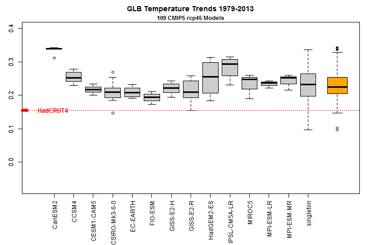
Figure 1 Modelled versus observed decadal global surface temperature trend 1979–2013
Temperature trends in °C/decade. Models with multiple runs have separate boxplots; models with single runs are grouped together in the boxplot marked ‘singleton’. The orange boxplot at the right combines all model runs together. The default settings in the R boxplot function have been used. The red dotted line shows the actual increase in global surface temperature over the same period per the HadCRUT4 observational dataset.
Transient climate response
Virtually all the projections of future climate change in AR5 are based on the mean and range of outcomes simulated by this latest CMIP5 generation of climate models (AOGCMs). Changes in other variables largely scale with changes in global surface temperature. The key determinant of the range and mean level of projected increases in global temperature over the rest of this century is the transient climate response (TCR) exhibited by each CMIP5 model, and their mean TCR. Model equilibrium climate sensitivity (ECS) values, although important for other purposes, provide little information regarding surface warming to the last quarter of this century beyond that given by TCR values.
TCR represents the increase in 20-year mean global temperature over a 70 year timeframe during which CO2 concentrations, rising throughout at 1% p.a. compound, double. More generally, paraphrasing from Section 10.8.1 of AR5 WG1,TCR can be thought of as a generic property of the climate system that determines the global temperature response ΔT to any gradual increase in (effective) radiative forcing (ERF – see AR5 WGI glossary, here ) ΔF taking place over a ~70-year timescale, normalised by the ratio of the forcing change to the forcing due to doubling CO2, F2xCO2: TCR = F2xCO2 ΔT/ΔF. This equation permits warming resulting from a gradual change in ERF over a 60–80 year timescale, at least, to be estimated from the change in ERF and TCR. Equally, it permits TCR to be estimated from such changes in global temperature and in ERF.
The TCRs of the 30 AR5 CMIP5 models featured in WGI Table 9.5 vary from 1.1°C to 2.6°C, with a mean of slightly over 1.8°C. Many projections in AR5 are for changes up to 2081–2100. Applying the CMIP5 TCRs to the changes in CO2 concentration and other drivers of climate change from the first part of this century up to 2081–2100, expressed as the increase in total ERF, explains most of the projected rises in global temperature on the business-as-usual RCP8.5 scenario, although the relationship varies from model to model. Overall the models project about 10–20% faster warming than would be expected from their TCR values, allowing for warming ‘in-the-pipeline’. That discrepancy, which will not be investigated in this article, implies that the mean ‘effective’ TCR of the AR5 CMIP5 models for warming towards the end of this century under RCP8.5 is in the region of 2.0–2.2°C.
Observational evidence in AR5 about TCR
AR5 gives a ‘likely’ (17–83% probability) range for TCR of 1.0–2.5°C, pretty much in line with the 5–95% CMIP5 model TCR range (from fitting a Normal distribution) but with a downgraded certainty level. How does that compare with the observational evidence in AR5? Figure 10.20a thereof, reproduced as Figure 2 here, shows various observationally based TCR estimates.
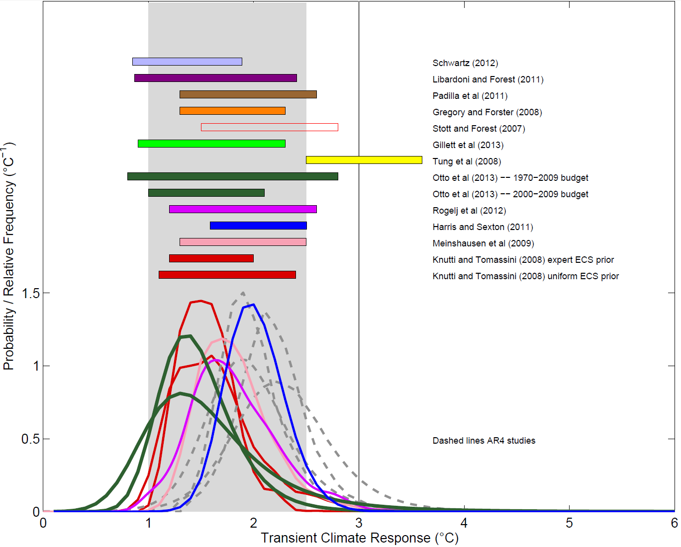
Figure 2. Reproduction of Figure 10.20a from AR5
Bars show 5–95% uncertainty ranges for TCR.[i]
.
On the face of it, the observational study TCR estimates in Figure 2 offer reasonable support to the AR5 1.0–2.5°C range, leaving aside the Tung et al. (2008) study, which uses a method that AR5 WGI discounts as unreliable. However, I have undertaken a critical analysis of all these TCR studies, here. I find serious fault with all the studies other than Gillett et al. (2013), Otto et al. (2013) and Schwartz (2012). Examples of the faults that I find with other studies are:
Harris et al. (2013): This perturbed physics/parameter ensemble (PPE) study’s TCR range, like its ECS range, almost entirely reflects the characteristics of the UK Met Office HadCM3 model. Despite the HadCM3 PPE (as extended by emulation) sampling a wide range of values for 31 key model atmospheric parameters, the model’s structural rigidities are so strong that none of the cases results in the combination of low-to-moderate climate sensitivity and low-to-moderate aerosol forcing that the observational data best supports – nor could perturbing aerosol model parameters achieve this.
Knutti and Tomassini (2008): This study used initial estimates of aerosol forcing totalling −1.3 W/m² in 2000, in line with AR4 but far higher than the best estimate in AR5. Although it attempted to observationally-constrain these initial estimates, the study’s use of only global temperature data makes it impossible to separate properly greenhouse gas and aerosol forcing, the evolution of which are very highly (negatively) correlated at a global scale. The resulting final estimates of aerosol forcing are still significantly stronger than the AR5 estimates, biasing up TCR estimation. The use of inappropriate uniform and expert priors for ECS in the Bayesian statistical analysis further biases TCR estimation.
Rogelj et al. (2012): This study does not actually provide an observationally-based estimate for TCR. It explicitly sets out to generate a PDF for ECS that simply reflects the AR4 ‘likely’ range and best estimate; in fact it reflects a slightly higher range. Moreover, the paper and its Supplementary Information do not even mention estimation of TCR or provide any estimated PDF for TCR.
Stott and Forest (2007): This TCR estimate is based on the analysis in Stott et al. (2006), an AR4 study from which all four of the unlabelled grey dashed-line PDFs in Figure 10.20a are sourced. It used a detection-and-attribution regression method applied to 20th century temperature observations to scale TCR values, and 20th century warming attributable to greenhouse gases, for three AOGCMs. Gillett et al. (2012) found that just using 20th century data for this purpose biased TCR estimation up by almost 40% compared with when 1851–2010 data was used. Moreover, the 20th century greenhouse gas forcing increase used in Stott and Forest (2007) to derive TCR (from the Stott et al. (2006) attributable warming estimate) is 11% below that per AR5, biasing up its TCR estimation by a further 12%.
In relation to the three studies that I do not find any serious fault with, some relevant details from my analysis are:
Gillett et al. (2013): This study uses temperature observations over 1851–2010 and a detection-and-attribution regression method to scale AOGCM TCR values. The individual CMIP5 model regression-based observationally-constrained TCRs shown in a figure in the Gillett et al. (2013) study imply a best (median[ii]) estimate for TCR of 1.4°C, with a 5–95% range of 0.8–2.0°C.[iii] That compares with a range of 0.9–2.3°C given in the study based on a single regression incorporating all models at once, which it is unclear is as suitable a method.
Otto et al. (2013): There are two TCR estimates from this energy budget study included in Figure 10.20a. One estimate uses 2000–2009 data and has a median of 1.3°C, with a 5–95% range of 0.9–2.0°C. The other estimate uses 1970–2009 data and has a median of slightly over 1.35°C, with a 5–95% range of 0.7–2.5°C. Since mean forcing was substantially higher over 2000–2009 than over 1970–2009, and was also less affected by volcanic activity, the TCR estimate based on 2000–2009 data is less uncertain, and arguably more reliable, than that based on 1970–2009 data.
Schwartz (2012): This study derived TCR by zero-intercept regressions of changes, from the 1896–1901 mean, in observed global surface temperature on corresponding changes in forcing, up to 2009, based on forcing histories used in historical model simulations. The mean change in forcing up to 1990 (pre the Mount Pinatubu eruption) per the five datasets used to derive the TCR range is close to the best estimate of the forcing change per AR5. The study’s TCR range is 0.85–1.9°C, with a median estimate of 1.3°C.
So the three unimpeached studies in Figure 10.20a support a median TCR estimate of about 1.35°C, and a top of the ‘likely’ range for TCR of about 2.0°C based on downgrading 5–95% ranges, following AR5.
The implication for TCR of the substantial revision in AR5 to aerosol forcing estimates
There has been a 43% increase in the best estimate of total anthropogenic radiative forcing between that for 2005 per AR4, and that for 2011 per AR5. Yet global surface temperatures remain almost unchanged: 2012 was marginally cooler than 2007, whilst the trailing decadal mean temperature was marginally higher. The same 0.8°C warming now has to be spread over a 43% greater change in total forcing, natural forcing being small in 2005 and little different in 2012. The warming per unit of forcing is a measure of climate sensitivity, in this case a measure close to TCR, since most of the increase in forcing has occurred over the last 60–70 years. It follows that TCR estimates that reflect the best estimates of forcing in AR5 should be of the order of 30% lower than those that reflected AR4 forcing estimates.
Two thirds of the 43% increase in estimated total anthropogenic forcing between AR4 and AR5 is accounted for by revisions to the 2005 estimate, reflecting improved understanding, with the increase in greenhouse gas concentrations between 2005 and 2011 accounting for almost all of the remainder. Almost all of the revision to the 2005 estimate relates to aerosol forcing. The AR5 best (median) estimate of recent total aerosol forcing is −0.9 W/m2, a large reduction from −1.3 W/m2 (for a more limited measure of aerosol forcing) in AR4. This reduction has major implications for TCR and ECS estimates.
Moreover, the best estimate the IPCC gives in AR5 for total aerosol forcing is not fully based on observations. It is an expert judgement based on a composite of estimates derived from simulations by global climate models and from satellite observations. The nine satellite-observation-derived aerosol forcing estimates featured in Figure 7.19 of AR5 WGI range from −0.09 W/m2 to −0.95 W/m2, with a mean of −0.65 W/m2. Of these, six satellite studies with a mean best estimate of −0.78 W/m2 were taken into account in deciding on the −0.9 W/m2 AR5 composite best estimate of total aerosol forcing.
TCR calculation based on AR5 forcing estimates
Arguably the most important question is: what do the new ERF estimates in AR5 imply about TCR? Over the last century or more we have had a period of gradually increasing ERF, with some 80% of the decadal mean increase occurring fairly smoothly, volcanic eruptions apart, over the last ~70 years. We can therefore use the TCR = F2xCO2 ΔT/ΔF equation to estimate TCR from ΔT and ΔF, taking the change in each between the means for two periods, each long enough for internal variability to be small.
That is exactly the method used, with a base period of 1860–1879, by the ‘energy budget’ study Otto et al. (2013), of which I was a co-author. That study used estimates of radiative forcing that are approximately consistent with estimates from Chapters 7 and 8 of AR5, but since AR5 had not at that time been published the forcings were actually diagnosed from CMIP5 models, with an adjustment being made to reflect satellite-observation-derived estimates of aerosol forcing. However, in a blog-published study, here, I did use the same method but with forcing estimates (satellite-based for aerosols) taken from the second draft of AR5. That study estimated only ECS, based on changes between 1871–1880 and 2002–2011, but a TCR estimate of 1.30°C is readily derived from information in it.
We can now use the robust method of the Otto et al. (2013) paper in conjunction with the published AR5 forcing best (median) estimates up to 2011, the most recent year given. The best periods to compare appear to be 1859–1882 and 1995–2011. These two periods are the longest ones in respectively the earliest and latest parts of the instrumental period that were largely unaffected by major volcanic eruptions. Volcanic forcing appears to have substantially less effect on global temperature than other forcings, and so can distort TCR estimation. Using a final period that ends as recently as possible is important for obtaining a well-constrained TCR estimate, since total forcing (and the signal-to-noise ratio) declines as one goes back in time. Measuring the change from early in the instrumental period maximises the ratio of temperature change to internal variability, and since non-volcanic forcings were small then it matters little that they are known less accurately than in recent decades. Moreover, these two periods are both near the peak of the quasi-periodic ~65 year AMO cycle. Using a base period extending before 1880 limits one to using the HadCRUT surface temperature dataset. However, that is of little consequence since the HadCRUT4 v2 change in global temperature from 1880–1900 to 1995–2011 is identical to that per NCDC MLOST and only marginally below that per GISS.
In order to obtain a TCR estimate that is as independent of global climate models as possible, one should scale the aerosol component of the AR5 total forcing estimates to match the AR5 recent satellite-observation-derived mean of −0.78 W/m2. Putting this all together gives ΔF = 2.03 W/m2 and ΔT = 0.71, which, since AR5 uses F2xCO2 = 3.71 W/m, gives a best estimate of 1.30°C for TCR. The best estimate for TCR would be 1.36°C without scaling aerosol forcing to match the satellite-observation derived mean.
So, based on the most up to date numbers from the IPCC AR5 report itself and using the most robust methodology on the data with the best signal-to-noise ratio, one arrives at an observationally based best estimate for TCR of 1.30°C, or 1.36°C based on the unadjusted AR5 aerosol forcing estimate.
I selected 1859–1882 and 1995–2011 as they seem to me to be the best periods for estimating TCR. But it is worth looking at longer periods as well, even though the signal-to-noise ratio is lower. Using 1850–1900 and 1985–2011, two periods with mean volcanic forcing levels that, although significant, are well matched, gives a TCR best estimate of 1.24°C, or 1.30°C based on the unadjusted AR5 aerosol forcing estimate. The TCR estimates are even lower using 1850–1900 to 1972–2011, periods that are also well-matched volcanically.
What about estimating TCR over a shorter timescale? If one took ~65 rather than ~130 years between the middles of the base and end periods, and compared 1923–1946 with 1995–2011, the TCR estimates would be almost unchanged. But there is some sensitivity to the exact periods used. An alternative approach is to use information in the AR5 Summary for Policymakers (SPM) about anthropogenic-only changes over 1951–2010, a well-observed period. The mid-range estimated contributions to global mean surface temperature change over 1951–2010 per Section D.3 of the SPM are 0.9°C for greenhouse gases and ‑0.25°C for other anthropogenic forcings, total 0.65°C. The estimated change in total anthropogenic radiative forcing between 1950 and 2011 of 1.72 Wm-2 per Figure SPM.5, reduced by 0.04 Wm-2 to adjust to 1951–2010, implies a TCR of 1.4°C after multiplying by an F2xCO2 of 3.71 Wm-2. When instead basing the estimate on the linear trend increase in observed total warming of 0.64°C over 1951–2010 per Jones et al. (2013) – the study cited in the section to which the SPM refers – (the estimated contribution from internal variability being zero) and the linear trend increase in total forcing per AR5 of 1.73 Wm-2, the implied TCR is also 1.4°C. Scaling the AR5 aerosol forcing estimates to match the mean satellite observation derived aerosol forcing estimate would reduce the mean of these two TCR estimates to 1.3°C.
So does the observational evidence in AR5 support its/the CMIP5 models’ TCR ranges?
The evidence from AR5 best estimates of forcing, combined with that in solid observational studies cited in AR5, points to a best (median) estimate for TCR of 1.3°C if the AR5 aerosol forcing best estimate is scaled to match the satellite-observation-derived best estimate thereof, or 1.4°C if not (giving a somewhat less observationally-based TCR estimate). We can compare this with model TCRs. The distribution of CMIP5 model TCRs is shown in Figure 3 below, with a maximally observationally-based TCR estimate of 1.3°C for comparison.
.

Figure 3. Transient climate response distribution for CMIP5 models in AR5 Table 9.5
The bar heights show how many models in Table 9.5 exhibit each level of TCR
.
Figure 3 shows an evident mismatch between the observational best estimate and the model range. Nevertheless, AR5 states (Box 12.2) that:
“the ranges of TCR estimated from the observed warming and from AOGCMs agree well, increasing our confidence in the assessment of uncertainties in projections over the 21st century.”
How can this be right, when the median model TCR is 40% higher than an observationally-based best estimate of 1.3°C, and almost half the models have TCRs 50% or more above that? Moreover, the fact that effective model TCRs for warming to 2081–2100 are the 10%–20% higher than their nominal TCRs means that over half the models project future warming on the RCP8.5 scenario that is over 50% higher than what an observational TCR estimate of 1.3°C implies.
Interestingly, the final draft of AR5 WG1 dropped the statement in the second draft that TCR had a most likely value near 1.8°C, in line with CMIP5 models, and marginally reduced the ‘likely’ range from 1.2–2.6°C to 1.0–2.5°C, at the same time as making the above claim.
So, in their capacity as authors of Otto et al. (2013), we have fourteen lead or coordinating lead authors of the WG1 chapters relevant to climate sensitivity stating that the most reliable data and methodology give ‘likely’ and 5–95% ranges for TCR of 1.1–1.7°C and 0.9–2.0°C, respectively. They go on to suggest that some CMIP5 models have TCRs that are too high to be consistent with recent observations. On the other hand, we have Chapter 12, Box 12.2, stating that the ranges of TCR estimated from the observed warming and from AOGCMs agree well. Were the Chapter 10 and 12 authors misled by the flawed TCR estimates included in Figure 10.20a? Or, given the key role of the CMIP5 models in AR5, did the IPCC process offer the authors little choice but to endorse the CMIP5 models’ range of TCR values?
.
[i] Note that the PDFs and ranges given for Otto et al. (2013) are slightly too high in the current version of Figure 10.20a. It is understood that those in the final version of AR5 will agree to the ranges in the published study.
[ii] All best estimates given are medians (50% probability points for continuous distributions), unless otherwise stated.
[iii] This range for Gillett et al. (2013) excludes an outlier at either end; doing so does not affect the median.


77 Comments
Re the boxplots in Figure 1:
“The default settings in the R boxplot function have been used.”
For those of us who are R-deprived, could you state the settings? For example, is the thick black horizontal line the mean or median?
Lance Wallace
“For those of us who are R-deprived, could you state the settings [of the R boxplot function]? For example, is the thick black horizontal line the mean or median?”
The thick black line is the median. The box ends are the 25% and 75% points of the distribution.
Nic, with the data from Figure 1, do you think you could plot the value of TCR vs. Temp?
I would like to know what the lineshape looks like
DocMartyn
I don’t have the data handy to plot what you suggest. But I can say that there is no significant dependence of simulated historical temperature increase (1850/1860 to 2001-05) on a model’s TCR, for the models analysed in Forster et al (2013, JGR).
Nic,
Regarding Otto 2013, any comments on aerosol uncertainty as described here as well as Carslaw et al., 2013 and OHC uncertainty as described in Trenberth and Fasullo, 2013 based on ORAS-4 estimates?
Yes. Karsten Haustein’s comments are wrong. I haven’t yet managed to get any answers out of the Carslaw team to some initial questions I have asked on their paper – I can’t replicate the one set of results that they provide sufficient data to be able to do calculate – let alone been able to analyse their work properly, so I don’t place significant weight on it at present.
ORAS-4 is not an observational OHC dataset, and anyway ocean heat uptake doesn’t come in to TCR estimates based on the AR5 formula.
@niclewis: Saying something is wrong doesn’t make it wrong. In essence, I stand by my comment (made before AR5 came out) linked above. You are also wrong in assuming that satellite derived (indirect) aerosol forcing estimates are more reliable than model estimates. They are not. Knowing that it’s not your area of expertise, I will have to reject your ill-advised assumptions regarding the aerosol forcing.
Karsten, OK, let’s take one of your statements in the linked comment and see if it’s right or not:
“Assuming it is balanced, one shouldn’t assume the decadal heat uptake in the reference period (1860-1879 in their case) to be positive (0.08W/m2). It’s quite a stretch for which they didn’t have a good reference (or justification for that matter). Assuming zero forcing in the reference period, I would rather set the heat content uptake to zero as well. Only GCM results can provide more reliable results. One would have to determine the fraction of the natural OHC at the beginning and at the end of the time interval in question, starting the simulation at least 500 years before.”
Actually, Otto et al. referenced Gregory et al. (2002) for 1860-79 ocean heat uptake (OHU). Its 0.16 W/m2 OHU estimate for 1861-1900, derived from AOGCM simulations, was halved to be conservative, following my doing so in my last December’s blog-published study. I agree a long simulation with natural forcings is needed. The one that Gregory used started in the year 1000.
Taking a very recent reference, the sea level rise data in Gregory et al (2013) supports a higher OHU estimate, of 0.25 W/m2, over 1860-79. Not that OHU affects TCR estimation using the energy budget method.
Re aerosol forcing, I think you are really implying that the AR5 expert authors were wrong to make a best estimate of -0.9 W/m2 total ERF in 2011, quite close to the six satellite-based estimates they took into account (mean -0.78 W/m2, median -0.85 W/m2). You appear to think that they should instead have come up with an estimate closer to the seven model based estimates that they also took into account (mean -1.28 W/m2, median -1.38 W/m2). Unlike you, the AR5 experts obviously think that the satellite-based aerosol forcing estimates are more reliable than model-based ones.
Nic, which observational datasets for aerosols do you recommend?
Hopefully Dr. Haustein will return to explain how it was proven (the declarative statement “they are not” implies proof) that the model estimates are more reliable than the indirect empirical estimates. In fact, I would like to see how something like that is proven under any set of circumstances!
Nic, let me briefly explain myself a bit clearer:
Re OHC as referenced in Gregory et al. (2002), not only am I well aware of their paper and what’s been done, but also do I stand by my earlier comment. It remains a stretch, as you compare modelled (for 1860-79) with observed OHU data. Make it apples to apples and take AOGCM OHU for start and end period. If you believe that your assumptions are robust, you are entitled to do so. I happen to be less convinced. That’s all.
But anyways, problem is, if I were to take the AR5 estimate for the last 30 years from 1980-2011 (arguably the most reliable, despite the fact that the last decade is still afflicted with considerable uncertainties), things have still to be consistent. Fig 8.20 in AR5 provides a total effective anthropogenic forcing of 0.95W/m2 for the specified period. The GISS trend is 0.16K/decade, which makes it roughly 0.5K. Using the effective forcing (for doubling) of 3.44W/m2, TCR is 1.8K. Natural forcing is small over that period, as solar and volcanic forcing tend to balance each other. I argue that aerosol forcing wasn’t negative (as assumed by the AR5 authors), which would bring TCR down to 1.6K. Still a bit off your 1.3K. While not entirely inconsistent, there is a considerable gap which has to be explained. Alternatively, following Fig 8.19 in AR5, the total forcing trend (natural+anthropogenic) between 1951-2011 is 0.3W/m2/decade, which makes it approx. 1.5W/m2. Temperature change is 0.65K, yielding a TCR of 1.5 (assuming effective radiative forcing). These are my benchmark numbers, based on AR5. The AR5-forcing of 1.72W/m2 for 1950-2011 which you are using seems to neglect changes in natural forcing.
Re overall aerosol forcing: While I tend to agree with the AR5 experts, they might have gone a tad too far. So what? Nowhere did I ever claim that they should have given more weight to the models. The one thing I didn’t know back in May was, that someone had already converted the aerosol forcing (as provided in Bellouin et al. 2013) into an effective aerosol forcing. I’m still not 100% sure how it has been done, but again, nowhere did I reject these estimates. I just happen to know that they are not as reliable as you think they are. You don’t need to believe me of course. Unlike you, I also do know that not all of the experts involved are also experts in remote sensing. Might therefore well be true that a few of them are indeed overestimating the validity of satellite products. Don’t get me wrong, I’m glad we have them, but it’s quite a way to go until they can be trusted blindly. Let me finally ask you one question: Are you aware of the numerous (poorly constrained) assumptions which have to be made in order to obtain the forcing from remote sensing products?
@Steve McIntyre: Sometimes it’s quite revealing who gets asked a question.
Karsten, you say
“It remains a stretch, as you compare modelled (for 1860-79) with observed OHU data.”
I (and Otto et al) were obliged to use modelled ocean heat uptake (OHU) in the second half of the nineteenth century as a proxy for observed data as there were no observations. What you should, IMO, be saying is that if the model used had a much higher sensitivity than the estimate derived from observations, then it would be appropriate to scale down its OHU estimate accordingly. And both I and Otto et al did so, to the extent of 50% from the 1860-1900 model estimate used in Gregory (2002), or 68% from the 1859-1882 model estimate in Gregory (J Clim 2013). Since the models involved have ECS values of 3 C or so, and TCRs of 1.8-2 C, even 50% is an over-conservative scaling down. To do as you suggest and used the unscaled OHU estimate from a sensitive model for the recent period would bias ECS and TCR estimation towards the high model sensitivity value. Surely that is obvious?
“… if I were to take the AR5 estimate for the last 30 years from 1980-2011 … Fig 8.20 in AR5 provides a total effective anthropogenic forcing of 0.95W/m2 for the specified period. The GISS trend is 0.16K/decade, which makes it roughly 0.5K. Using the effective forcing (for doubling) of 3.44W/m2, TCR is 1.8K. Natural forcing is small over that period, as solar and volcanic forcing tend to balance each other. I argue that aerosol forcing wasn’t negative (as assumed by the AR5 authors), which would bring TCR down to 1.6K.”
Yes, it is unclear whether aerosol forcing has become more negative over the last 30 years. But your figures are wrong. The AR5 best estimate of the change in anthropogenic forcing over 1980-2011 is 1.04 W/m2, with a linear trend based change of 1.01 W/m2. Where did you get your 0.95 W/m2 figure from? As it happens, that error of yours largely cancels out with your use of 3.44 W/m2 for a doubling of CO2 concentration, when in fact the AR5 Figure 8.20 etc. forcing data are based on a value of 3.71 W/m2.
But I wouldn’t attempt to estimate TCR over a 30 year period using crude surface temperature data, because of the large impact of multidecadal internal variability. Over 1980-2011 the Delsole et el (J. Climate, 2011) estimate the forced trend in sea-surface temperature (SST) as fairly constant at 0.122 K decade over 1977-2008, during which the AR5 forcing trend with constant aerosol forcing was 0.516 W/m2 per decade. That implies a TCR of 0.88 C for SST. Scaling that up by the ratio of global to SST temperature of 1.30 (per HadCRUT4/HadSST3) raises the TCR estimate to 1.14 C, far below your 1.6 C. That looks rather low to me. I suggest the lesson probably is: don’t try to estimate TCR or ECS over periods of only a few decades.
“The AR5-forcing of 1.72W/m2 for 1950-2011 which you are using seems to neglect changes in natural forcing.”
Of course it is an anthropogenic-only forcing, since I was comparing it with an anthropogenic-only temperature change. An apples-to-apples comparison, yes?
” Are you aware of the numerous (poorly constrained) assumptions which have to be made in order to obtain the forcing from remote sensing products?”
Yes, I am aware it is a tricky job. But the AR5 aerosol forcing uncertainty range far exceeds the stated uncertainty ranges for most satellite-based observational estimates, so it seems to me to take plenty enough account of the uncertainties involved – quite possibly more than is needed, particularly given the constraints provided by inverse estimates of aerosol forcing.
Nic,
Re the OHU discussion: I’m afraid I don’t have to add much. If you think you can learn something from what you’ve done, fine with me.
Re 1980-2011: As referenced, my 1980-2011 forcing (0.95W/m2) is taken from Fig 8.20 (Chapter 8) and it is undoubtedly the effective radiative forcing (ERF). Your forcing (1.04W/m2 ) is from Fig SPM.5, but unfortunately, it seems to be only the non-adjusted forcing as total aerosol forcing is only -0.82W/m2 rather than the central estimate of -0.9W/m2. On top of that, it is only the anthropogenic forcing, while we need the total forcing (i.e. a slight negative solar forcing term for 1980-2011 has to be added). Doing so, brings both figures in very good agreement. Given that Fig 8.20 provides ERF, the forcing for doubling should be 3.44W/m2. With dT of 0.5K, TCR is 1.81. Taking the forcing from SPM.5 and combining it with 3.71W/m2, TCR is 1.78K. Again, very good agreement here. I’m actually not so sure that I’m the one who is mistaken.
Apart from that, I’m not here to debate ocean oscillations. We won’t agree on that one anyways. Note however, that regionally aerosol forcing has dramatically changed at multidecadal timescales. That’s all I have to say.
Re 1950-2011: It’s only now that I see what you actually did. Apologies for the slight confusion on my part here. You are using the temperature attributed to anthropogenic forcing from Chapter 10. Fair enough. Interesting though that you suddenly seem to fancy GCM results, given that all these attribution studies are based on CMIP5 data (scaled to match HadCRUT4). That also explains the small difference when it comes to the forcing estimates. The best estimate for temperature change (1950-2011) attributable to natural forcing is zero, while the actual natural forcing is estimated to be slightly negative (due to declining solar activity) as pointed out in my previous comment. A minor inconsistency which indicates that any detection and attribution study is afflicted with uncertainties (not surprisingly). No reason for me to dismiss them. After all, I’m certainly happy to note that you put trust in GCM results. In fact, Fig 10.4 provides the required scaling factors (to match HadCRUT4) that could allow us to deduce the corresponding “true” model TCR. The multimodel mean seems to be 1.8K. With the multimodel scaling factor of 0.8 (Fig 10.4b), TCR comes down to 1.44. An extremely rough (quick and dirty) guess, but one which is fairly consistent with my earlier estimates.
Re remote sensing: I tend to disagree on the uncertainty range. Given that you won’t convince me of the opposite, we should leave it at that.
Excuse my ignorance but isn’t it rather fraught estimating climate sensitivity by dividing the measured temperature change over a given period by the estimated change in CO2-based forcing?
The biggest problem I see is that we have no way of knowing that the change in temperature is entirely due to the change in forcing from CO2. Some of it could be natural variation, up or down and there could be other forcings too.
If the change in temperature from change in CO2 over a given period is x and the change in temperature from otter sources is y and the change in forcing from CO2 is z, what we want to know is x / z but what you’re actually calculating is (x + y) / z where the magnitude of y could be close to (or possibly even exceed) x and is unknown. Surely then this result can only give us a very rough, “ball park” figure – certainly not a figure with two decimal places.
Or am I missing something?
Nicholas
“The biggest problem I see is that we have no way of knowing that the change in temperature is entirely due to the change in forcing from CO2”
In the usual method, the measured change in mean temperature between two periods is divided by the change in estimated total forcing from all sources, not just CO2.
Natural variation is indeed a source of uncertainty. The effect of shorter term variations can be minimised by making each of the two periods long – typically one to four decades and trying to get a similar El Nino – El Nina balance in both periods. Balancing their volcanic activity levels is also important. The effect of a quasi-cyclical multidecadal variations can be minimised by matching the positions of the two periods in the cycle. And maximising the difference in mean temperature between the two periods dilutes the effect of internal variations. Hence taking one period in the second half of the nineteenth century and the other as recently as possible.
Accuracy is clearly not even to a single decimal place in TCR in terms of standard error, but stating results to two d.p. is helpful to avoid large rounding uncertainty.
nic, thanks for clarifying and that all makes sense but what about long-term natural warming/cooling trends such as those which may have caused the Roman Warm Period, Medieval Warm Period, Little Ice Age and so on? While they are somewhat controversial there is a certain amount of evidence that natural variability can create centuries-long trends which ultimately shift temperatures by several degrees. So for example some warming included in the TCR calculation may be “recovery” from the LIA which may not be due to a known forcing at all – my understanding is that nobody really knows what causes these natural fluctuations. So surely the uncertainty for a temperature delta of 0.5K going into this formula must be large. It’s hard to see how you can get a result with a 95% CI that doesn’t overlap both low and high TCR estimates and thus fails to help narrow down the answer at all…
One of the really remarkable points Nic makes here is that, just using numbers from the IPCC report itself, and applying their own formula for transient climate response, an estimate of around 1.3C is unavoidable. Yet most of the models they employ have TCR’s of 1.6 or higher, and quite a few are even above 2, implying way too much sensitivity to CO2 emissions. Yet the IPCC goes on to say things like “There is very high confidence that models reproduce the general features of the global-scale annual mean surface temperature increase over the historical period, including the more rapid warming in the second half of the 20th century, and the cooling immediately following large volcanic eruptions.” (Ch 9 p. 3). The whole summary section of Ch 9 gives the impression that models and observations are beautifully in alignment. Something’s gotta give here.
Ross McK.
“Something’s gotta give here.”
I suspect that they are hoping that the next few years will show an uptick in surface temps, and save them. It’s the bitter-ender method of fighting – refuse to surrender, and pray for a miracle.
Interesting analysis. Only continued divergence from reality will force the modelers to fix the models. A few have already undergone a substantial reduction in diagnosed sensitivity (eg GISS Model E-R). Another decade should force the hand of most modeling groups. Which is not to say I think the models will then accurately represent reality; cloud feed backs will probably be adjusted only enough for the model projections to fall in the range of just barely plausible.
There are many ways a model could be adjusted. Lets classify them into two types
1. Adjustments which lower TCR but not ECS. These are mechanisms of delay. Catastrophe is not cancelled, merely postponed.
2. Adjustments which lower TCR and ECS both. Under these kinds of adjustments the Catastrophe may need to be cancelled.
Faced with a choice of adjustment methods what logic will be used in choosing which one to apply? Am I being too cynical in expecting that every possible type 1 adjustment will be explored in depth before type 2 adjustments are even considered.
Ya well, higher aerosol offsets and ‘hidden’ deep ocean heat uptake are getting a lot of attention lately (both ‘type 1 adjustments’). But these things are only delaying tactics against the inevitable; reality will not be denied for ever.
you are not taking into account the inextinguishable creative spark the species. They will never concede, but simply invent new ways to keep the ball in the air. But their antics will isolate them from serious science, as has already occurred to a large extent.
ECS may be most likely a second order effect in terms of expected temperature rise and therefore policy. I don’t see the need for biased motive seeking even if it were assumed that ocean heat uptake numbers are likely to be revised in the future.
This is a graph of the changes in global optical depth at 550 nm from 1970 to the end of 2012; which is a very good measure of atmospheric aerosol light-scattering.
What is note worthy is how little aerosols have been flung into the atmosphere over the last decade or so. Note that this is the same period where we have observed he ‘pause’ in global warming. This aerosol get-out-of-jail-free card for the modelers is pretty much defunct for the last 12 years.
Dependence on ‘adjusted’ temperature records still worries me greatly. Although not representative of the globe, there are many, many records from Australia that have been studied in detail here. The official Bureau of Met line is that positive adjustments balance negative just nicely, but we do not find that. We find cooling of older years to give an exaggerated trend since about 1880 or so. The correctness or otherwise of the adjusted global record is so basic to estimates of TCR and ECS.
I sometimes wonder if mismatches in CMIP5 and earlier comparisons are due in part to more rigid physics meeting less rigid T adjustments. Even in the satellite era, there are differences between RSS and UAH, some of which can be large, see a regional comparison at http://www.warwickhughes.com/blog/?p=2496
(I realise that this comment is not helpful because I have not given a solution to the problem – apologies).
Wow Nic. Herculean work continues I see. Do you have a job? Amazing amounts of detail poured through on every paper to an extent that is very unusual. If you get a CS degree, they will pay you high 6 figures for that work and you can do it in your spare time. I think you can get one of those on line these days.
Then again, they might pay you the same money not to do it!
What happened here?
“Note that the PDFs and ranges given for Otto et al. (2013) are slightly too high in the current version of Figure 10.20a. It is understood that those in the final version of AR5 will agree to the ranges in the published study. “
Very interesting analysis. A few months ago I looked at something similar (although I did not examine the other TCR estimate papers as you did here), trying to figure out how the SPM could say that > 2K warming was “likely” and “more likely than not” with high confidence for the RCP6.0 and RCP4.5 scenarios, when the most up-to-date TCR estimates (Otto et al., 2013 in particular) implied quite the opposite:
As far as I can tell, these statements stem from the CMIP5 projections, and the (seemingly mistaken) idea that the somewhat-arbitrary-expert-selected-TCR-range matches up with the CMIP5 TCR range, and that this apparent match endorses more specific aspects of the CMIP5 TCR distribution.
Troy,
Yes, I like your 17 October blog article.
I’m not sure to what extent the AR5 Chapter 10 authors would regard the 1-2.5 C TCR range as expert-selected rather than (as it should in principle be) based on observational evidence. The wording of the final paragraph of Section 10.8.1 implies it is based primarily on observational evidence.
Whilst it would have been difficult for the Ch. 10 authors not to have been influenced by the CMIP5 TCR range, that influence may mainly have operated indirectly through observational TCR studies that were consistent with the similar CMIP3/AR4 TCR range being more likely to be published, and given weight to in Chapter 10. However, it would no doubt in any case have been very awkward for the Ch. 10 authors to propose a TCR range that conflicted substantially with the CMIP5 TCR range.
Nic Lewis rocks! Thank you so much… Massive contradictions within the IPCC report… Perfectly objective exposition. I stand in awe.
Nic,
Nice article. And credit to Troy above, who did get there a bit before you on the issue of the flawed comparison of the pdf’s from observation and model.
I can’t really fault you for using the same assumptions as the IPCC to demonstrate the irregularity of its conclusions.
On a higher plain, however, making any TCR estimate without a clear statement of assumptions about the multidecadal oscillations seems to me to be bad science.
There are now an embarrassing richness of papers which confirm the existence of quasi-60-year cycles in temperature and other climate indices, going back many centuries. There is an embarrassing lack of credible papers which explain root cause.
If they are caused by “internal mode” – an internal redistribution of heat, then simply ignoring them in an energy budget calculation renders such calculation highly dependent on the time-period chosen for the analysis. Choosing 1950 to 1979, for example, gives a very different answer from choosing 1970 to 1999.
On the other hand, if the cycles are caused by, or if they induce, an unaccounted-for flux forcing, then the total forcing on the system will be under- or over-estimated. In particular, the total forcing in late 20th century would be under-estimated, giving rise to overestimation of TCR.
I can reproduce an estimate of TCR of 1.34 which matches ocean heat content and surface temperature data available from 1955 to present day. Hindcasting this model match reveals that the model temperature neatly lops off the peaks and troughs of the previous multi-decadal cycles in the observed temperature data. In fact the model result looks very similar to the matches achieved by the AOGCMs when their results are averaged over a few runs. I am fairly confident that this TCR represents an upper bound on the modal estimate (before accounting for uncertainties in the input data series).
I have been trying for several weeks to pull an article together on this for Lucia, including the indications of some external flux forcing, but keep getting distracted by my wife telling me that I should be doing something useful (instead).
Paul,
Thanks.
I agree about the importance of multidecadal oscillations, and I don’t ignore them. One can use the Internal Multidecadal Pattern (IMP) shown in Fig. 4 of Delsole et al (J. Climate, 2011) as a guide to selecting base periods to match the final period used in energy budget estimation of TCR and ECS. The IMP was high over 1995-2011; it was also fairly high over 1859-1882, the base period I use. It was also fairly high from the late 1920s through to 1960. So rather than taking a fixed 65 year periodicity and using 1923–1946 for my shorter baseline TCR estimate, there is an arguemnt for using 1930-1960. Doing so gives almost identical TCR estimates.
Your point about the possibility of the cycles actually being in forcing (presumably mediated through changes in clouds) rather than in redistribution of heat (primarily between the ocean and atmosphere) is interesting. If that is the case, then energy budget ECS estimates as well as TCR estimates would be affected. In principle internal changes in heat distribution should not affect such ECS estimates, since an increase in energy flow into the ocean would be accompanied by a depression of surface temperature (a favourite explanation for the current “hiatus”). So a comparison of the relationship of energy budget TCR and ECS estiamtes over different states of the IMP might throw light on which explanation for multidecadal oscillations is valid. However, I’m not sure whether that decent records of heat uptake (or its counterpart, satellite-measured TOA radiative imbalance) are yet long enough to reach solid conclusions. I shall be very interested in your article at Lucia’s blog – let me know when you post it. You can tell your wife that others think you are doing useful and important cliamte science work!
Nic, for the detection of the IMP you refer to ftp://wxmaps.org/pub/delsole/dir_ipcc/dts_jclim_2010.pdf . Maybe one can have a clearer impression of the impact of multidecadal oscillations when calculating the stability indecies ( R²) of running linear trends with a length as noted in the diagram: http://www.dh7fb.de/reko/bestgiss.gif ( Data: GISS). With shorter Trends than 70 years you get some oscillation in R² with clear maxima and minima of R² and a length of the “periode” of about 60 years. So it’s clear, that for a calculation of TCR only intervals of more than 70 years are useful because the shorter ones have not enough stability over time.
Frank,
Yes, that’s one way to expose the periodicity.
In practice, any half-way decent spectral analysis, including a straight Fourier analysis, a bandpass filter or elemental mode decomposition, will expose the cycles in the modern temperature datasets. That’s not where the big challenge lies IMO.
The first challenge is to demonstrate that the cycles are not just persistent autoregressive stochastic wanderings. With only two and a half cycles available in the modern global series, there is no statistical test which confirms unambiguously that they are “predictably recurrent”. To confirm predictable recurrence requires the use of longer-term temperature records or the use of long-term proxy records. See, for example, http://depts.washington.edu/amath/research/articles/Tung/journals/Tung_and_Zhou_2013_PNAS.pdf
So far, at least, the mainstream modelers have rejected the evidence for predictable recurrence. The GCM’s treat these cycles as stochastic natural variation, and cannot reproduce the phasing – that’s official. One consequence is that the cycles from 1850 to around 1960 disappear when averages of temperature are taken over several GCM runs, so the peaks and troughs of the observed temperature series are “lopped off”. Thereafter the model average tracks the temperature gain for the late 20th century, natural plus “forced” – and continues to climb after the predictable cycle peak around the end of the 20th century.
My specific concern, relevant to Nic’s article, is that many applications of energy balance or energy budget models actually make de facto assumptions which are similar to the GCM modelers, and hence produce an upper bound on, rather than most likely, estimates of transient sensitivity. As Nic indicates, it is possible that the error is minimised by comparing energy balance sheets over periods when the multidecadal variations are “in the same phase”. Fair enough. There is however still a problem with mathematical coherence in doing this, which is one of the things I am trying to write up at the moment.
In short form, under the assumption that there are no external fluxes other than the predefined forcings and feedbacks, I believe that we can eliminate the likelihood that the “transfer and storage” mechanism for net heat redistribution is between ocean and atmosphere on several grounds. Latent heat flux is in the wrong direction to add heat flux to the mixed layer when needed. Sensible heat flux is almost in phase between atmosphere and ocean, as evidenced by temperature movements (no source and sink available). Regional surface distribution doesn’t work either since local variations are almost in phase with each other globally (by latitude and by ocean basin) within a 10-year timespan. This leaves only sensible heat movement within the oceans from somewhere to the surface mixed layer. This is not a global diffusion process; it is likely to be controlled entirely by local or regional changes in the deep convective regions and in the equatorial Pacific. (See Kosaka and Xie 2013.)
If this is valid, then we do not expect to see the oscillations in any valid measure of total ocean heat content, since the internal heat fluxes are self-cancelling. However, since the oscillations are not visible in the forcing series (apart from an artful artifactual kink around 1950) but are included in the temperature feedback, then mathematically the oscillations should be visible in the net total ocean heat flux. A clear contradiction. So we either accept the mathematical incoherence of the energy balance model, or we reject the assumption that the cycles have no external flux forcing. (Or you can reject my logic that the net flux movement must be entirely internal to the oceans.)
Additional to the above is the fact that long-term MSL data shows crystal clear evidence of 60 year cycles. So can we conclude that there must be an unaccounted-for external flux forcing? Maybe.
Frank,
Thanks for sharing this graph. I concur with your conclusion that estimating TCR over intervals separated by less than 60-70 years (or trends over periods of at least that length) is not reliable.
In principle, if multidecadal natural cycles in surface temperature are caused by fluctuations in ocean heat uptake, then if OHU (or its counterpart, TOA radiative imbalance) can be measured accurately it would be feasible to estimate ECS over a shorter period than 60-70 years. But I’m not sure it would be a good idea to attempt that – ECS might vary over the multidecadal cycle.
Paul,
Thanks for your detailed comments. I agree that the Tung and Zhou paper is helpful in that it considers a much longer period than the Delsole one. I tend to cite Delsole as it identifies the post 1850 IMP/AMO contribution quite well.
As you may know, some UK Met Office GCM modellers (Booth et al, 2012) have sought to explain the AMO as the result of changes in aerosol forcing. Zhang et al (2013) contained a pretty devastating criticism of that explanation.
As you say, multidecadal quasi-cycles without a predictable period cause problems for TCR estimation. If those fluctuations are the counterpart of changes in OHU, it may be that first estimating ECS, taking account of those changes, offers a better route. TCR could then be derived from ECS using an OHU measure (e.g., assuming a mixed layer + diffusive ocean) that was estimated over a long period, to iron out the effects of multi-decadal cycles.
Re your argument about the net flux movement being internal to the ocean, why does that prevent it causing fluctuations if global surface temperature? If cold deep water upwells and is warmed by (and cools) the atmosphere, or there is more mixing of warm surface water with cold deeper water (by increased isopycnal transport or whatever), that would depress the surface temperature and equate to a higher rate of OHU. Or are you saying that you don’t think the global rate of downwards heat transport in the ocean can change much?
It is certainly possible that multidecadal changes in the distribution of surface temperature are causing changes in global cloud forcing, which in turn cause fluctuations in global mean surface temperature. I think is what you are suggesting? But is there any decent evidence for that?
Nic,
Thanks for the additional comments.
Re aerosol forcing – I agree it was total nonsense.
It doesn’t, Nic. That’s not the problem. The problem is one of coherence in application of an energy balance. Definitionally, the net downward flux at TOA = Forcing – lambda*T. Assume the secular forcing is constant or zero, and let us consider the part of the oscillation when surface temperature is increasing. If the surface temperature increases because of (solely) internal ocean heat flux, then we will see a decrease in net incoming radiation – a net cooling of the upper ocean mixed layer plus atmosphere to space in net terms. At the same time, the surface mixed layer is displaying a heat gain which tracks SST – which heat comes by assumption from the deeper ocean. The heat flux from the deeper ocean to the mixed layer must be greater in magnitude than the radiative loss from the planet in order to support net heat gain by the mixed layer. In summary, the heat flux into the mixed layer is greater in amplitude than, and out of phase with, the TOA radiative flux – the latter is cooling when the former is heating and vice versa. So far this is OK, but now consider what happens when we make the common assumption in energy balance models that the integral of the net TOA flux must all end up as ocean heat. The ocean heat flux into the mixed layer is exactly equal to the ocean heat flux out of the deep (under this model), so these fluxes should be self cancelling in any sum of total ocean heat content. The only thing that should be left visible is the net radiative flux due to surface temperature change. But this radiative flux is 180 degrees out of phase with the temperature oscillation, as explained above. So when we plot total OHC, we expect to see the oscillations 180 degrees out of phase with temperature – cooling at the temperature peaks – but we don’t; we see the opposite. The total heat flux moves in phase with temperature using the (very) limited data we have available. For a longer term proxy dataset, have a look at Figure 3 here:-http://www.psmsl.org/products/reconstructions/jevrejevaetal2008.php
Note that the MSL is a proxy for total heat and so its derivative should reflect flux. The flux oscillation is almost exactly in phase with the temperature oscillations and 180 degrees out of phase with what we should expect under the assumption that the oscillations are driven entirely by internal fluxes.
I believe that this is one source of unaccounted for forcing, but I am fairly sure that it is induced by ENSO. I know that you have looked at Forsetr and Gregory 2006 in terms of total feedback and uncertainty. If you havn’t done so, I would strongly recommend that you have a close look at the results obtained for SW and LW separately. The LW shows a range of feedbacks from small positive to very large negative. The SW shows a huge “positive feedback” – a forcing in disguise.
I do not believe that this cloud albedo change is the trigger for the oscillations. I think that the oscillations are controlled by another unaccounted for flux which has the correct periodicity – one which has been measured for a very long time, but which has to date been largely ignored by climate science. I will remain mysterious until I have written it up properly.
Correction.
I wrote: “When we plot total OHC”, when I meant to write
“When we plot the derivative of total OHC, we expect to see the oscillations 180 degrees out of phase with temperature.”
Sorry.
Paul,
Thanks. I agree that the SL reconstruction you cite supports your argument, but it’s unclear to me whether the SL data is accurate/reliable enough to establish it for certain. Whether ocean heat content data supports your argument or not over 1960-2000 depends on which dataset you look at. But since the late 1990s surface temperature has been pretty flat whilst the ocean heat content datasets show a continuing rise.
The Forster and Gregory 2006 SW surface temp. vs TOA radiation relationship is statistically insignificant in all or most cases, so I’m not sure how much it shows. But it could indeed represent a forcing. The Lindzen and Choi lagged regression papers are quite interesting on the forcing vs feedback issue, as you are probably aware.
I look forward to reading your piece at Lucia’s.
Paul, Nic… did you notice this paper: http://www.pmel.noaa.gov/people/gjohnson/OHCA_1950_2011_final.pdf about OHCA? It seems to be interesting because when one selects a climatology without too much “infill” due to the fuzziness of the early data ( b4 Argo) the record of OHCA gets another face… as you can see in Fig.4 of the paper. Any impact to discussion about IMV vs. Forcing?
Frank, Thanks, I’d missed that, although I’ve read a previous paper of theirs on the influence of climatology on OHC timeseries. I’ll look at their new one.
Thanks for the reference, Frank, which I had not seen.
If we accept the 0-1800m data series as (a) true and (b) representative of the total OHC, then it suggests that net flux (the derivative of the curve shown in Fig 4)is roughly tracking surface temperature. Over the period shown, it starts at a high, decreases to a low value, climbs to a peak around 2001 and then decreases after that – pretty well in phase with the multidecadal temperature oscillation which achieved an oscillatory high in the 40’s and just after the turn of the century. This is the exact opposite in phase of what we would expect if the surface temperature oscillation was caused by internal ocean flux movement, if you accept my previous argument. So applying my previous logic, we reject the hypothesis that the oscillations are caused by heat redistribution within the ocean and look for an external flux.
If I were a climate scientist then I would describe this a robust result(TM)since all of the OHC reconstructions seem, at least, to show the same peak in flux around the turn of the century.
The real problem, Frank, is that the data are poo – despite the best efforts of the authors. There is practically no information on the deep ocean >900m prior to the last decade, and the little that is available is heavily weighted towards the N Hemisphere (see Figure 2 in the same paper). To make matters worse, there is no certainty that a depth limit of 1800m allows us to capture the total relevant heat movement – it may be pulsing from even deeper ocean.
So basically, the data are just too uncertain to draw any trustworthy conclusions.
Nic, Paul: I did some calculations to redo Nic’s analysis for TCR. I only used the “Forcing-table” from http://www.climatechange2013.org/images/uploads/WGIAR5_WGI-12Doc2b_FinalDraft_Chapter08.pdf wich I translated in a numerical file http://kauls.selfhost.bz:9001/uploads/ipcc5forc2.txt and the T-anomaly from GISS since 1880.
The most important step is to notice, that the T-response is the response to the sum of forcings. That’s why I recalculated the net-forcing into synthetic CO2-ppm data (C) with the formula C= 278,24* e (exp P/5,35) where P is the forcing in W/m² from the table. Now one can recalculate the TCR ( which is NOT the response to CO2 but the Response to ALL forcings). The result for the periode I selected (2006…2010 vs. 1941…1945 with 5y Means of both: ppm and T) is about 1.7. Now you can also calculate the percentage of CO2-forcing, it’s about 80%. So in the end the TCR due to CO2 is in my eyes also 1.4, redone in another way. Maybe this kind of operation has some advantages, because one can select the percentages of all forcings on TCR. If somebody wants to replicate: don’t bother sending an email: dh7fb at gmx.de. And one more feature: When you bring the netforcing of the IPCC- table ( best to use the net forcing without volcano) and die Tanomaly into a scatter-diagram and make a figure of the residuals to linear trend…you can see also very clear the IMV and note, that something is missing..either a forcing or an internal variation. Many mainproblems of todays climate research poke in this table…fascinating!
I don’t know if anyone noticed here Sherwood et.al (2014). In the paper a positive tropical cloud feedback is postulated which leads to CS 4…5. (see also: http://www.eurekalert.org/pub_releases/2013-12/uons-ncs121913.php with the headline “Cloud mystery solved: Global temperatures to rise at least 4°C by 2100”. Anyway, in the paper is no empirically evidence from observations included. So I tried this one: Have a look at fig. 3 and 4 where the you can see that the lower altitude drying effect is located at an area -30…30N over the oceans. So I looked at the SST ( HadISST1) there and found, that the saisonal variation is about 1,1 K between April ( max.) and August ( min). If the “Sherwood-effect” is at work one should assume that the slope of the SST of Aprils is higher than the slope of the SST of Augusts over the years 1900…2013 due to the positive feedback “found” in the paper. This is not the case: http://www.dh7fb.de/reko/tropminmax.gif . So my question: is such an observation able to confirm or falsify the described effect in http://www.nature.com/nature/journal/v505/n7481/full/nature12829.html ?
Nic, Paul,
For what it’s worth, the more I have looked at energy balances the more convinced I have become that long term cyclical behaviors could be driven by changes in albedo (changes in relatively low clouds in particular). The potential influence of clouds on energy balance is large compared to GHG forcing, and it would not take a big change in cloud albedo (positive or negative) to greatly exceed the magnitude of concurrent changes in GHG forcing. I just don’t know of any relevant cloud/albedo data to examine.
Steve,
There is some useful information here:-
http://isccp.giss.nasa.gov/products/onlineData.html
You need to browse to find the “FD Online data and images” which shows a marked reduction in upwelling shortwave between 1982 and 1999 followed by an increase. Numerous studies – some referenced therein – have suggested it was largely due to cloud albedo. What is not known because of the short length of record is whether this is a typical and recurrent component of the quasi 60-year temperature cycles.
The first diagram is a nice summary.
Of course, the models will never be precise and there will always be unavoidable random errors. If so, you would expect roughly half to be too warm and the other half too cool. But they are all too warm.
This demonstrates that the greatest error component is consistent and not random. Surely this shows that the basic AGW theory, on which the models are firmly based, is wrong.
Chris
Steve: this post is technical and interesting and doesn’t bear on “basic AGW theory”. Blog policy discourages readers from trying to discuss “basic AGW theory” as all blog comments quickly become identical.
Chris Wright: “This demonstrates that the greatest error component is consistent and not random. Surely this shows that the basic AGW theory, on which the models are firmly based, is wrong.”
This doesn’t seem obvious to me. The AGW theory could be sound but the processes it establishes may not have the proportional significance they ascribe to it in the presence of other not-well-understood natural processes. Doesn’t that also make sense to you?
Steve: quite so. no more debate on this OT point please.
Awesomely short debate there – well done John and (for the upteenth time) our host. As for Nic, a precision strike that stands on its own merits. I look forward to the interaction with Haustein and others.
My first visit here.
Well, having read these ‘climate’ blogs for some time, it seems apparent (if you ignore the ex cathedra pronouncements of the IPCC and the CAGW Team and look at the actual climate data) that as actual data accumulates the climate sensitivity to ACO2 is asymptotically approaching zero.
Jim Cripwell will, justifiably, feel vindicated.
I’m sure that Nick Stokes could make a useful contribution here.
Re: Don Keiller (Dec 10 10:23), Sometimes surety (or certainty) can be misplaced — as this post most assuredly made clear.
Nic,
Thanks for your (and Troy’s) analysis.
Faced with the facts that the ECS and TCR observationally-based estimates were some 40% below the CMIP5 model estimates, and, as you note, that other impacts scale with the surface temperature, the IPCC was in a bind.
As we predicted (http://www.cato.org/blog/ipcc-chooses-option-no-3), they basically chose to praise the Emperor’s new duds. Their other options weren’t so palatable!
-Chip
Steve McIntyre wrote “Nic, which observational datasets for aerosols do you recommend?”
I generally use the time series for total aerosol effective radiative forcing (ERF) in Table AII.1.2 of AR5 WG1 Annex II, which is based on their ‘expert’ best (median) estimate of -0.9 W/m2 in 2011, and scale it by an alternative recent observational aerosol estimate. For that I normally take the mean (-0.78 W/m2) of the six satellite-based estimates given in Table 7.4 of AR5, which vary from -0.45 to -0.95 W/m2. As the table caption makes clear, these estimates are corrected for ERFari (aerosol direct ERF) and for the longwave component of ERFari+aci (aerosol direct plus indirect ERF) when these are not included, hence they are mostly not fully observational. But most of the uncertainty concerns ERFaci, which all the satellite-based studies do include.
There are some other satellite-based studies shown in Figure 7.19. Including those would lower the mean of the satellite studies to -0.65 W/m2. But the AR5 authors had reasons for selecting the six studies that they chose.
The other obvious source of observational estimates of recent aerosol ERF is inverse studies, often of ECS with aerosol forcing being estimated alongside it. Only those that use temperature data that is resolved latitudinally, at least by hemisphere, should be considered. Any omitted forcings with a similar fingerprint will be included in the estimation and need to be deducted, Black carbon on snow-and-ice being the obvious one. Even after such adjustments, the inverse studies generally give aerosol forcing estimates in line with or below the mean satellite-based estimate of -0.78 W/m2. Candidate studies to consider are Aldrin et al (2012), Ring et al (2012), Lewis (2013) and Libardoni & Forest (2013 – correction to 2011). Aldrin used an AR4 based expert prior for aerosol forcing, which pushed up its best estimate.
Nic, I was hoping that you could point me to specific online links that give monthly or quarterly aerosol estimates? Preferable ones that are consistent with IPCC usage.
Steve, there’s some aerosol data available at http://climexp.knmi.nl/select.cgi?id=someone@somewhere&field=tomsai , but only from 1980-2001. And various aerosol optical depth etc datasets are at http://gacp.giss.nasa.gov/data_sets/. There’s also a PDF document with a list of datasets and URLs available there. http://aeronet.gsfc.nasa.gov/new_web/aerosols.html is another dataset access point. But this is almost all recent data.
I haven’t used any of the above, as they don’t provide the long term data I need. That is mainly estimated from emissions. Various papers show estimates graphically. I can’t find any online links for download at present. I use the IPCC report estimated time series as they are authoritative and cover the whole period of relevance.
Steve and everybody who needs the latest forcing data: The IPCC- data from http://www.climatechange2013.org/images/uploads/WGIAR5_WGI-12Doc2b_FinalDraft_AnnexII.pdf in Tab. A II 1.2. in a .txt – file for calculations: http://kauls.selfhost.bz:9001/uploads/ipcc5forc2.txt from 1870 on.
Steve: yes, thanks for this. But these have already translated aerosol data into forcing, which is helpful but only part of the story. I presume that these come from some public data on actual measurements in micrograms per something or other. CO2 values are regularly reported in ppm and data can be examined. I was wondering what was the equivalent for aerosols. The IPCC data goes to 2011 and we’re now in 2013. What is the best source for current data?
Nic – I did not see any discussion of the water-vapor feedback. I would think the most likely explanation for the consistent high-side bias is that the assumptions around this parameter are invalid.
Tom C
This article wasn’t really about why the CMIP5 models have as high a sensitivity as they do, hence the lack of discussion of feedbacks. You may very well be right that water-vapor feedback is part of the explanation, but differences in cloud feedbacks may account for rather more of the model – observational discrepancy.
A first assumption of GHG warming would invoke a uniform warming all over the globe as CO2 in particular is a well mixed gas. This does not seem to happen. Warming attributed to GHG seems to be observed in some regions more intensely than in others.
So there is spatial variability.
There is increasing documentation of a temperature cycle of 60 years or so, with mention of more cycles of different periods.
So there is temporal variability.
The value of ECS and/or TCR might be dependent on the overall temperature for the period being calculated or physical factors.
So there is feedback variability.
Estimates of global temperature vary between adjusters, for a given place and time.
So there is measurement variability.
One should correctly estimate the overall precision and bias errors from these 4 types of variables, before proceeding to calculate sensitivity factors. The reason is that the uncertainty of the sensitivity estimate cannot be smaller than the combined errors of its component parts, which remain unknown until measured and stated.
I have not done a formal error analysis, but in a similar vein, I would be surprised if surface sea temperature measurements were adequately representative to discern any trends for the periods quoted above. If observations are restricted to ARGO for deeper water temperatures, I would be surprised that any measurement of OHC could yet be derived because of inadequate temporal and spatial coverage and possible biases.
In short, there seems to be a lack of formal demonstration that much of the relevant work is not proceeding entirely within an envelope of large errors, within which trends are largely meaningless.
I periodically ask this question, which again may be a measure of my ignorance. There is one other potential source of variability–sensitivity itself. As a non-scientist, I may be failing to see something very obvious, but I actually see no reason to assume that atmospheric sensitivity should be a fixed value, either as TCR or equilibrium. I hope someone will eventually enlighten me on this.
Tom Fuller, I too would have the same question, framed in the same way as you have framed it.
It is part of a broader question concerning just how predictably mechanistic the earth’s climate system is in responding to changes in forcings.
Tomas Milanovic has a nice answer to Tom’s question at the end of the ‘Hearing: A factual look at the relationship between weather and climate’ thread, at Judy’s Climate Etc. judithcurry.com
============
RE:Steve: this post is technical and interesting and doesn’t bear on “basic AGW theory”.
It does seem to bear on the ‘basic model programming’ doesn’t it? IE: increased CO2 emissions = increased temperatures. Most/all other parameters are secondary and therefore less/insignificant even independent of time scales. However, this seems to be only on a global scale.
Has there been no attempt at climate modeling for more regional or at least meaningful areas where we know certain climate conditions exist? I’m thinking where observations are immediate and constant, would this not allow more immediate and constant adjustments and re-programming of models? Would working out the kinks locally not be easy/faster? Thereby helping both the understanding and programming of larger scale models?
I’m among those that have no doubt that what we’re spewing into the air has far more impact locally/regionally than globally.
I can’t help but think more research into the local implications would be of far more use to far more people than the bi-monthly ‘it’s worse than we thought’ global implication dittos IE: from agriculture to seasonal industries.
the estimated contribution from internal variability being zero
Uh-huh. Do tell. More likely it is 100%.
Apparently there are people here who can read a technical post like this and not have their heads spin while doing it. I am not one of those. I think it’s great that such people exist (“Oh brave new world, that has such people in it!”), and it makes me grateful indeed for SM’s typical posts, which a non-insider like me can comprehend to some extent at least.
I’ve got my own crappy model which fits forcings and responses. It’s a derivative of the basic exponential decay model with the difference being that my model’s relative response to a pulse can decelerate. Anyway, my fits for the RCP4.5 and RCP6.0 model means both give a R^2 of 0.999 and a TCR ~2C. I also get a TCR ~2C when fitting to HadCRUT4.
https://sites.google.com/site/climateadj/cmip5-tas-emulation
Disclamer: I have no reason to believe my method is better than anything discussed here. Probably just another flawed model.
Steve McIntyreNic Lewis wrote “We can now use the robust method of the Otto et al. (2013) paper in conjunction with the published AR5 forcing best (median) estimates up to 2011, the most recent year given. The best periods to compare appear to be 1859–1882 and 1995–2011. These two periods are the longest ones in respectively the earliest and latest parts of the instrumental period that were largely unaffected by major volcanic eruptions. Volcanic forcing appears to have substantially less effect on global temperature than other forcings, and so can distort TCR estimation.”Steve,Nic,Great article but I have an issue with two points in this analysis.
One in the quote above, you rely on the argument that volcanic forcing has less effect than other forcings. If so then that is strong evidence that the climate models built on the assumption that the change in forcing times the climate sensitivity equals the change in temperature. The entire global warming theory is built on the house of cards that all forcings are equal. I think that implies that the climate sensitivity to other forcings is as low as it is for volcanic forcings.
The second issue with these estimated of climate sensitivity is that they are comparing sensitivity to a temperature data set that is unreliable. Between the errors in accounting for UHI, sighting issues, and adjustments for buckets and time of day we cannot accept that change between your two time periods being measured in your report to be accurate. If the adjustments and errors double or triple the temperature change between the two measurement periods then the climate sensitivity would be a half to a third of what your method would find.
Twas Nic Lewis wot wrote it.
Theodore
Global climate models are not built on the ASSUMPTION that the change in global temperature equals forcing times climate sensitivity for forcings other than CO2 (for which this follows from the definition of sensitivity, assuming linearity – which is found to hold). Rather, it is found that in climate models this relationship pretty well holds for almost all forcings other than volcanism, black carbon on snow and aerosol forcing. So the conclusion you draw is invalid.
The global surface temperature dataset is imperfect, but IMO it is most unlikely to be overstated by a factor of anything like two over the last 100+ years.
Nic,
I may have missed something but I thought the lower sensitivity to volcanoes was due to integration time. Leaving aside black carbon on snow, of which I have no knowledge, what is the rationale for a lower sensitivity to sustained aerosol forcing?
bill_c,
“what is the rationale for a lower sensitivity to sustained aerosol forcing?”
Actually, it’s higher, not lower, for aerosol forcing as it is for black carbon on snow. It’s better understood in terms of the effective forcing – once the atmosphere but not surface temperatures have fully adjusted to increase aerosols – being higher than the pure radiative forcing. It is a complex subject. If you want to understand it, I recommend reading Chapter 8 of the IPCC AR5 WGI report (and Ch. 7 for more in depth information about aerosols).
The fact that nobody within the scientific community seems to even contemplate removing the overly-warm end of the climate model ensemble is bizarre.
…….. even when they can see that those models are inconsistent with observations.
Can any of these models replicate the global temperature singularity of 1940 when, in a single year, change from +0.5C to -0.5C occurred? This is a critical test that all models must pass in order to be taken seriously. See my website.
In my view, the figure 3 in this post is wrong; as it is said that observed TCR is 1.3 ºC, but in my pdf:
https://docs.google.com/file/d/0B4r_7eooq1u2VHpYemRBV3FQRjA
I explain why an appropriate estimation of ECS (and of TCR) must require centuries of data collection.
Is it possible to contact Mr. Steve McIntyre? I would like to talk with him about my pdf.
Antonio, go to the home page of CA. At the upper left you will see a link for contact information.
May I please intrude on a very interesting article and a fascinating discussion. While blog policy rightly discourages reference AGW theory could the same policy also encourage those future bloggers, who continue to ignore that policy, to distinguish between AGW and GAGW. There are many of us who, while doubting CAGW, are happy to go along with AGW. There is a difference.
Nic
Please don’t refer to RCP8.5 as “the business-as-usual case”. It is in fact the extreme case – covering the worst consequences scientists have ever devised.
The four RCPs are all hypotheticals. They are designed to cover all forcing ranges mentioned in the literature. Unlike the SRES scenarios, the range does NOT exclude outliers.
In comparison with SRES the BAU case would be RCP4.5.
7 Trackbacks
[…] Does the observational evidence in AR5 support its/the CMIP5 models’ TCR ranges? […]
[…] missing out on it. In case you haven’t noticed, Nic Lewis has established himself as a top expert on climate model performance. I don’t believe anyone in the climate community is turning out work to the quality and […]
[…] Lewis has a post Does the observational evidence in AR5 support its CMIP5 models’ TCR ranges? In the comments, McKitrick summarizes […]
[…] https://climateaudit.org/2013/12/09/does-the-observational-evidence-in-ar5-support-itsthe-cmip5-model… […]
[…] For more about this see the IPCC, Estimates of TCR are an active subject of research. Estimates are dropping, indicating less warming effect from CO2. See this example from the June 2013 issue of Nature Geoscience, and one of the author’s survey of the current estimates. […]
[…] [2] https://climateaudit.org/2013/12/09/does-the-observational-evidence-in-ar5-support-itsthe-cmip5-model… […]
[…] Pagina 24-27 en 34-43 van ons rapport gaan hierover, plus de appendix, plus een uitgebreid blogbericht op Climate Audit dat alle relevante schattingen voor de Transient Climate Response (TCR) nog eens onder de loep […]