A guest post by Nic Lewis
This new Nature Climate Change paper[i] by Drew Shindell claims that the lowest end of transient climate response (TCR) – below 1.3°C – in CMIP5 models is very unlikely, and that this suggests the lowest end of model equilibrium climate sensitivity estimates – modestly above 2°C – is also unlikely. The reason is that CMIP5 models display substantially greater transient climate sensitivity to forcing from aerosols and ozone than to forcing from CO2. Allowing for this, Shindell estimates that TCR is 1.7°C, very close to the CMIP5 multimodel mean of ~1.8°C. Accordingly, he sees no reason to doubt the models. In this connection, I would note (without criticising it) that Drew Shindell is arguing against the findings of the Otto et al (2013) study,[ii] of which he and myself were two of the authors.
As with most papers by establishment climate scientists, no data or computer code appears to be archived in relation to the paper. Nor are the six models/model-averages shown on the graphs identified there. However, useful model-by-model information is given in the Supplementary Information. I was rather surprised that the first piece of data I looked at – the WM-GHG (well-mixed greenhouse gas) global forcing for the average of the MIROC, MRI and NorESM climate models, in Table S2 – is given as 1.91 W/m², when the three individual model values obviously don’t average that. They actually average 2.05 W/m². Whether this is a simple typo or an error affecting the analysis I cannot tell, but the apparent lack of care it shows reinforces the view that little confidence should be placed in studies that do not archive data and full computer code – and so cannot be properly checked.
The extensive adjustments made by Shindell to the data he uses are a source of concern. One of those adjustments is to add +0.3 W/m² to the figures used for model aerosol forcing to bring the estimated model aerosol forcing into line with the AR5 best estimate of -0.9 W/m². He notes that the study’s main results are very sensitive to the magnitude of this adjustment. If it were removed, the estimated mean TCR would increase by 0.7°C. If it were increased by 0.15 W/m², presumably the mean TCR estimate of 1.7°C would fall to 1.35°C – in line with the Otto et al (2013) estimate. Now, so far as I know, model aerosol forcing values are generally for the change from the 1850s, or thereabouts, to ~2000, not – as is the AR5 estimate – for the change from 1750. Since the AR5 aerosol forcing best estimate for the 1850s was -0.19 W/m², the adjustment required to bring the aerosol forcing estimates for the models into line with the AR5 best estimate is ~0.49 W/m², not ~0.3 W/m². On the face of it, using that adjustment would bring Shindell’s TCR estimate down to around 1.26°C.
Additionally, the estimates of aerosol forcing in the models that Shindell uses to derive the 0.3 W/m² adjustment are themselves quite uncertain. He gives a figure of -0.98 W/m² for the NorESM1‑M model, but the estimate by the modelling team appears to be -1.29 W/m². Likewise, Shindell’s figure of -1.44 W/m² for the GFDL-CM3 model appears to be contradicted by the estimate of -1.59 W/m² (or -1.68 W/m², dependent on version), by the team involved with the model’s development. Substituting these two estimates for those used by Shindell would bring his TCR estimate down even further.
In any event, since the AR5 uncertainty range for aerosol forcing is very wide (5–95% range: -1.9 to -0.1 W/m²), the sensitivity of Shindell’s TCR estimate to the aerosol forcing bias adjustment is such that the true uncertainty of Shindell’s TCR range must be huge – so large as to make his estimate worthless.
I’ll set aside further consideration of the detailed methodology Shindell used and the adjustments and assumptions he made. In the rest of this analysis I deal with the question of to what extent the model simulations used by Shindell can be regarded as providing reliable information about how the real climate system responds to forcing from aerosols, ozone and other forcing components.
First, it is generally accepted that global forcing from aerosols has changed little over the well-observed period since 1980. And most of the uncertainty in aerosol forcing relates to changes from preindustrial (1750) to 1980. So, if TCR values in CMIP5 models are on average correct, as Shindell claims, one would expect global warming simulated by those models to be, on average, in line with reality. But as Steve McIntyre showed, here, that is far from being the case. On average, CMIP5 models overestimate the warming trend between 1979 and 2013 by 50%. See Figure 1, below.
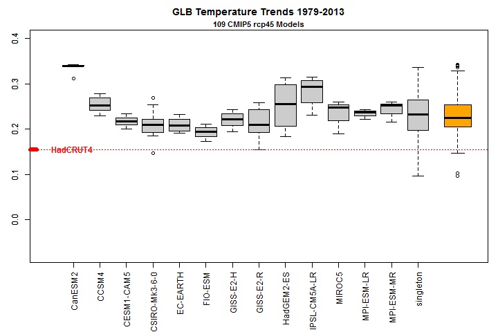
Figure 1: Modelled versus observed decadal global surface temperature trend 1979–2013
Temperature trends in °C/decade. Virtually all model climates warmed much faster than the real climate over the last 35 years. Source: https://climateaudit.org/2013/09/24/two-minutes-to-midnight/. Models with multiple runs have separate boxplots; models with single runs are grouped together in the boxplot marked ‘singleton’. The orange boxplot at the right combines all model runs together. The default settings in the R boxplot function have been used; the end of the boxes represent the 25th and 75th percentiles. The red dotted line shows the actual trend in global surface temperature over the same period per the HadCRUT4 observational dataset. The 1979–2013 observed global temperature trends from the three datasets used in AR5 are very similar; the HadCRUT4 trend shown is the middle of the three.
.
Secondly, the paper relies on the simulation of the response of the CMIP5 models to aerosol, ozone and land use changes being realistic, and not overstated. Those components dominate the change in total non-greenhouse gas anthropogenic forcing over the 1850-2000 period considered in the paper. Aerosol forcing changes are most important by a wide margin, and land use changes (which Shindell excludes in some analyses) are of relatively little significance.
For its flagship 90% and 95% certainty attribution statements, AR5 relies on the ‘gold standard’ of detection and attribution studies. In order to separate out the effects of greenhouse gases (GHG), these analyses typically regress time series of many observational variables – including latitudinally and/or otherwise spatially distinguished surface temperatures – on model-simulated changes arising not only from separate greenhouse gas and natural forcings but also from other separate non-GHG anthropogenic forcings. The resulting regression coefficients – ‘scaling factors’ – indicate to what extent the changes simulated by the model(s) concerned have to be scaled up or down to match observations. There is a large literature on this approach and the associated statistical optimal fingerprint methodology. The IPCC, and the climate science community as a whole, evidently considers this observationally-based-scaling approach to be a more robust way of identifying the influence of aerosols and other inhomogeneous forcings than the almost purely climate-model-simulations-based approach used by Shindell. I agree with that view.
Figure 10.4 of AR5, reproduced as Figure 2 below, shows in panel (b) estimated scaling factors for three forcing components: natural (blue bars), GHG (green bars) and ‘other anthropogenic’ – largely aerosols, ozone and land use change (yellow bars). The bars show 5–95% confidence intervals from separate studies based on 1861–2010, 1901–2010 and 1951–2010 periods. Best estimates from the studies using those three periods are shown respectively by triangles, squares and diamonds. Previous research (Gillett et al, 2012)[v] has shown that scaling factors based on a 1901 start date are more sensitive to end date than those starting in the middle of the 19th century, with temperatures in the first two decades of the 20th century having been anomalously low, so the 1861–2010 estimates are probably more reliable than the 1901–2010 ones.
Multimodel estimates are given for the 1861–2010 and 1951–2010 periods (“multi”, at the top of the figure). The best estimate scaling factors for ‘other anthropogenic’ over those periods are respectively 0.58 and 0.61. The consistency of the two best estimates is encouraging, suggesting that the choice between these two periods does not greatly affect results. The average of the two scaling factors implies that the CMIP5 models analysed on average exaggerate the response to aerosols, ozone and other non-greenhouse gas anthropogenic forcings by almost 70%. However, the ‘other anthropogenic’ scaling factors for both periods have wide ranges. The possibility that the true scaling factor is zero is not ruled out at a 95% confidence level (although zero is almost ruled out using 1951–2010 data alone).
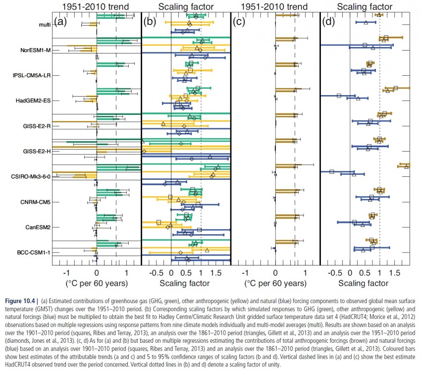 Figure 2: Reproduction of Figure 10.4 of IPCC AR5 WGI report
.
The individual results for models used by Shindell are of particular interest.
The first of the five individual CMIP5 models included in Shindell’s analysis, CanESM2, shows negative scaling factors for ‘other anthropogenic’ over all three periods – strongly negative over 1901–2010. The best estimates for its GHG scaling factor are also far below one over both 1861–2010 and 1951–2010. So it would be inappropriate to place any weight on simulations by this model. In Figure 1, it is CanESM2 that shows the greatest overestimate of 1979-2013 warming.
The second CMIP5 model in Shindell’s analysis, CSIRO-Mk3-6-0, shows completely unconstrained scaling factors using 1901–2010 data, and extremely high scaling factors for both GHG and ‘other anthropogenic’ over both 1861–2010 and 1951–2010 – so much so that the GHG scaling factor is inconsistent with unity at better than 95% confidence for the longer period, and at almost 95% for the shorter period. This indicates that the model should be rejected as a representation of the real world, and no confidence put in its simulated responses to aerosols, ozone or any other forcings.
The third of Shindell’s models, GFDL-CM3, is not included in AR5 Figure 10.4.
The fourth of Shindell’s models, HadGEM2, shows scaling factors for ‘other anthropogenic’ averaging 0.44, with all but the 1901–2010 analyses being inconsistent with unity at a 95% confidence level. The best defined scaling factor, using 1861–2010 data, is only 0.31, with a 95% bound of 0.58. So HadGEM2 appears to have a vastly exaggerated response to aerosol, ozone etc. forcing.
The fifth and last of Shindell’s separate models, IPSL-CM5A-LR, is included in Figure 10.4 in respect of 1861–2010 and 1901–2010. The scaling factors using 1861-2010 data are much the better defined. They are inconsistent with unity for all three forcing components, as are those over 1901-2010 for natural and GHG components. That indicates no confidence should be put in the model as a representation of the real climate system. The best estimate scaling factor for ‘other anthropogenic’ for the 1861-2010 period is 0.49, indicating that the model exaggerates the response to aerosols, ozone etc. by a factor of two.
Shindell also includes the average of the MIROC-CHEM, MRI-CGCM3 and NorESM1-M models. Only one of those, NorESM1-M, is included in AR5 Figure 10.4.
To summarise, four out of six models/model-averages used by Shindell are included in the detection and attribution analyses whose results are summarised in AR5 Figure 10.4. Leaving aside the generally less well constrained results using the 1901–2010 period that started with two anomalously cold decades, none of these show scaling factors for ‘other anthropogenic’ – predominantly aerosol and to a lesser extent ozone, with minor contributions from land use and other factors – that are consistent with unity at a 95% confidence level. In a nutshell, these models at least do not realistically simulate the response of surface temperatures and other variables to these factors.
A recent open-access paper in GRL by Chylek et al,[vi] here, throws further light on the behaviour of three of the models used by Shindell. The authors conclude from an inverse structural analysis that the CanESM2, GFDL-CM3and HadGEM-ES models all strongly overestimate GHG warming and compensate by a very strongly overestimated aerosol cooling, which simulates AMO-like behaviour with the correct timing – something that would not occur if the models were generating true AMO behaviour from natural internal variability. Interestingly, the paper also estimates that only about two-thirds of the post-1975 global warming is due to anthropogenic effects, with the other one-third being due to the positive phase of the AMO.
In the light of the analyses of the characteristics of the models used in Shindell’s analysis, as outlined above, combined with the evidence that Shindell’s aerosol forcing bias-adjustment is very likely understated and that his results’ sensitivity to it makes his TCR estimate far more uncertain than claimed, it is difficult to see that any weight should be put on Shindell’s findings.
.
[i] Drew T. Shindell, 2014, Inhomogeneous forcing and transient climate sensitivity. Nature Climate Change. doi:10.1038/nclimate2136, available here (pay-walled).
[ii] Otto, A., F. E. L. Otto, O. Boucher, J. Church, G. Hegerl, P. M. Forster, N. P. Gillett, J.Gregory, G. C. Johnson, R. Knutti,N. Lewis,U. Lohmann, J.Marotzke,G.Myhre, D. Shindell, B Stevens and M. R. Allen, 2013. Energy budget constraints on climate response. Nature Geosci., 6: 415–416.
[iii] A.Kirkevag et al, 2013, Aerosol-climate interactions in the Norwegian Earth System Model-NorESM1-M. GMD .
[iv] M.Salzmann et al, 2010: Two-moment bulk stratiform cloud microphysics in the GFDL AM3 GCM: description, evaluation, and sensitivity tests. ACP.
[v] Gillett N.P., V. K. Arora, G. M. Flato, J. F. Scinocca, K. von Salzen, 2012: Improved constraints on 21st-century warming derived using 160 years of temperature observations. Geophys. Res. Lett, 39, L01704, doi:10.1029/2011GL050226
[vi] P Chylek e al., 2014. The Atlantic Multidecadal Oscillation as a dominant factor of oceanic influence on climate. GRL.


54 Comments
Very convincing case provided by Nic, as usual. I was confused by this:
“Aerosol forcing changes are most important by a wide margin, and land use changes (which Shindell excludes in some analyses) are of relatively little significance.”
I was not sure if this means that the paper is making this assumption, Nic is making the assumption, or it is now a universally accepted fact.
Matt, thanks for your comment. You asked what I meant by:
“Aerosol forcing changes are most important by a wide margin, and land use changes (which Shindell excludes in some analyses) are of relatively little significance.”
This is based both on what is stated in the paper and on the changes in estimated forcing over 1850-2000, the analysis period in Shindell’s paper, given in AR5.
The paper mentions forcing changes for aerosols of -0.9 W/m2, for ozone +0.27 W/m2 and for land use -0.085 W/m2. It also has model average forcing changes of -1.13 W/m2 for aerosols and +0.32 W/m2 for ozone. Per AR5 the estimated change in total aerosol forcing is -0.74 W/m2, that in total ozone forcing is +0.29 W/m2 and that in land use -0.11 W/m2. All these relationships support my statement.
Unfortunately what Nic Lewis describes here is not untypical of “establishment” climate scientists where in Nic’s words for the paper he has analyzed for us here: “The extensive adjustments made by Shindell to the data he uses are a source of concern.” and “no data or computer code appears to be archived in relation to the paper” and “the sensitivity of Shindell’s TCR estimate to the aerosol forcing bias adjustment is such that the true uncertainty of Shindell’s TCR range must be huge – so large as to make his estimate worthless” and the seemingly arbitrary to cherry picked climate models used in Shindell’s analysis.
I think to be kind to some of these efforts to prove a point, that needs not saying, is that after a hard analysis such as Nic here provides, what we have left are results with uncertainty limits from floor to ceiling.
I should add that as the relationship of estimated TCR to adjusted aerosol forcing is non-linear, the range is smaller on the downside, and a 0.25 W/m² rather than 0.15 W/m² increase in Shindell’s aerosol forcing adjustment is required to bring his TCR estimate down to 1.35 C. But the Shindell TCR estimate range corresponding to the AR5 5-95% total aerosol forcing range is unbounded on the upside: it is approximately 0.95 C to infinity.
However, this is all somewhat academic because the fingerprint-based detection and attribution results in AR5 show that models used by Shindell to estimate his enhanced response factor E poorly represent the real world response to aerosol, ozone and land use forcings.
Nic, thanks for this.
did Shindell report the before and after forcings used in his study?
Steve, do you mean the aerosol forcing before and after adjustment? He did report that, although I can’t make total sense of what he says.
Shindell says F_aerosols are reduced from the ACCMIP mean of -1.2 W/m2 to match the AR5 best estimate of -0.9 W/m2. The models he uses have a weighted mean aerosol forcing of -1.13 W/m2 per his Table S2, but I think he ignores that – the F_aerosols figure just seems to be used for his TCR equation. Working backwards from his -0.64 W/m2 main text figure for aerosols, ozone and land use combined, and subtracting 0.317 W/m2 for ozone (weighted mean from Table S2) and -0.085 W/m2 for land use per the SI text implies an aerosol forcing figure of -0.87 W/m2, which doesn’t quite agree to the -0.90 W/m2 AR5 best estimate. Nor does it equal -1.13 + 0.30 = 0.83 W/m2. But they are all close. Maybe I’ve missed something.
Or was it some other forcings you were after?
I don’t have the paper itself and was assuming that there would be a data file showing forcing by year, as opposed to discursively in the text. WHat year are the text figures applicable to?
Also, presumably the underlying aerosol data is not in wm-2, but in some other unit. What real-time aerosol measurement data does Shindell reconcile to? (If any.)
Nic Re: “Shindell TCR estimate range . . .is unbounded on the upside”
Shindell’s TCR upper bound does not sound realistic compared to nature and physics. Contrast : Doiron et. al 2014 Fig. 5.1 p 74 who constrain Transient Climate Sensitivity (TCS) by observation. Further:
PS to my 4:48 AM post:
The non-linearity of the TCR estimate to aerosol forcing also means that a 0.49 W/m2 total adjustment would bring the TCR estimate down to about 1.4°C, not 1.26°C (which was based on a simple scaling of Shindell’s sensitivity analysis).
Very nice analysis.
I am wondering about GISS-E2-H. This is not one of the models overestimating GHG and compensating with overestimated aerosol effects, according to Chylek et al (assuming that the GISS-E2-H1 is the same as GISS-E2-H above). If my assumption is correct, do you know what caused such poorly constrained yellow bars in IPCC Figure 10.4 for this model?
No, I’m unsure why that is. The attribution papers involved comment on GISS-E2-H poor regression results but give no suggested explanation for them. I know that some climate scientists don’t think the GISS model is very good, but I’m not an expert on GCMs and I wouldn’t want to hazard a guess. Sorry.
I have attempted to model climate models and observed temperature series with ARMA models and then compare the red/white noise that these models generate from simulations. Of the CMIP5 climate models with at least 5 runs, the GISS models have noise characteristics most like those observed for the earth. My comparison does not compare the deterministic trend differences due GHGs, aerosols, etc. I did not assume that the trends were linear and used a spline smooth to find the residuals for model fitting.
Nic – first sentence edit- lowest/highest.
Sorry, I don’t follow your comment “Nic – first sentence edit- lowest/highest.” Can you clarify?
in the first sentence of your post, you use the word “lower” twice. I believe you meant to use “lower” once and “higher” once.
Thanks, Nic.
Statement by Drew Shindell:
Click to access sap_comment_pnnl_study.pdf
The last paragraph, in which he speaks for “all scientists,” is particularly troubling.
Thanks Nic for this detailed analysis…
From the first moment climate models used aerosols as “explanation” of the 1945-1975 flat/cooling trend with increasing CO2 emissions, I have suspected that this only was a scapegoat to explain the then “pause”.
There is a huge offset between the sensitivity for aerosols and the sensitivity for CO2, which makes it possible to retrofit the temperature curve of the past century with any climate sensitivity you like to have. But that makes that practically all models now run into troubles to follow the current “pause”, those with the highest sensitivity the most…
“I think to be kind to some of these efforts to prove a point, that needs not saying, is that after a hard analysis such as Nic here provides, what we have left are results with uncertainty limits from floor to ceiling.”
The uncertainty limits are so large that one can be certain?
I would be mighty impressed if they came up with a model that was correct with natural variability, antroproghenic effects(both on climate and the DATA)?
I mean to say, how on Earth are they going to get models that work the way they keep changing the DATA?
” it is difficult to see that any weight should be put on Shindell’s findings.”
Wanna bet?
Nic,
Very thorough analysis! – but I have a different question for you.
There is going to be an endless arguments about the exact contributions of aerosols, other GHGs, black carbon etc. when deriving TCR from observations because we are following the model centric viewpoint. Likewise any low value of TCR will always be criticized because it has failed to properly take into account this or that forcing within a GCM. This is all because TCR has been defined as follows.
I only realized during the discussion on Ed Hawkins that for CMPI5 this means when the NET forcings are equal to the modeled forcing of doubling CO2 alone (3.7 W/m2).
Lets call this definition TCR(M). TCR(M) cannot be measured from experimental data and we are wasting our time trying. TCR(M) can only me “derived” from the results of a GCM.
Instead I would propose a new definition of TCR.
This definition TCR(E) can be measured by experiment. It is simply the average temperature rise when CO2 levels reach 560ppm. It can be essentially measured today. This definition removes the non-CO2 anthropogenic effects (aerosols, methane, soot etc.) and avoids getting trapped by the model centric view. These effects are essentially anthropgenic feedbacks jus like climate feedbacks – increased H2O.
In all other branches of physics models make predictions and experiments then test the models. Why should climate science be different?
Clive,
I agree with your sentiments, but the problem is that in reality there are many drivers of surface temperature change – isolating just the effect of CO2 is not practical. However, if one converts the total effects of all greenhouse gases, aerosols, etc. into an equivalent increase in CO2 concentration (by reference to their effective radiative forcing RF, that from a doubling of CO2 being F2xCO2), then what you suggest would be pretty much in line with the generic definition of TCR in Section 10.8.1 of AR5 WGI:
“TCR was originally defined as the warming at the time of CO2 doubling (i.e., after 70 years) in a 1% yr–1 increasing CO2 experiment (see Hegerl et al., 2007b), but like ECS, it can also be thought of as a generic property of the climate system that determines the global temperature response ΔT to any gradual increase in RF, ΔF, taking place over an approximately 70-year time scale, normalized by the ratio of the forcing change to the forcing due to doubling CO2, F2×CO2: TCR = F2×CO2 ΔT/ΔF”
Nic,
I don’t think you quite understood what I was suggesting. You cannot “measure” effective forcing. You can measure CO2 levels in the atmosphere and you can measure the rise in surface temperatures. For everything else you need models. CO2 levels are also an indirect measure of methane emissions and aerosol emissions since they are all related to fossil fuel usage and to the human activity enabled by fossil fuels (such as intensive farming, chemical industry etc.) So why not aim for a simple separation between theoretical physics (models) and experimental physics (measurements) ? Otherwise climate science models are basically unfalsifiable.
Human aerosols are only going to be significant with China and India using more and more coal. We still don’t know if they are eventually going to have anti-pollution policies. Correct me if I’m wrong, it doesn’t take too much time for aerosols to get out of the stratosphere (or atmosphere, which was it?). The effect is quite instantaneous (a few years, IIRC). And ozone will be for the most part outlawed starting from 2015.
Therefore aerosols or ozone aren’t a feedback or “are related to fossil fuel usage”. It is something different altogether.
You can measure (theoretically) aerosol levels and ozone. And perhaps there is some analysis I never heard of that can separate the forcings. Maybe some short-term signal analysis.
Daniel,
Why complicate things ? Natural variations in aerosols from volcanoes should average out over time. The goal should be to measure the warming caused by anthropogenic doubling of CO2. So why don’t we do exactly that ? If indeed you do just that then you get TCR = 1.7C using the current data for a CO2 doubling to 560ppm. see here – so a further 0.9C of warming by 2100.
It is only measuring ECS that you have to rely on the models see here
Sorry wrong ECS link try this one instead
Newbie question: I understand that TCR is typically calculated from 280 ppm.
AND,
AR5 WG1 RCP 4.5 scenario assumes that we hit 750-800ppm by the end of the century. On that pace *IF* TCR is 1.8, and we start from today (400ppm), if we hit 800ppm in 2090 (~1%/year), would we expect temps to be 1.7 degrees higher than 2015 temps, with ECS still to work itself out over the future? Is that a legitimate way of reading TCR? Is that what this table is trying to show?
Or does TCR ONLY work as a transitory estimate of CO2 doubling starting from 280?
Or is this table projecting that TCR in 2080 in RCP4.5 will be a TOTAL of 1.8, and since temp has ALREADY gone up 1.0 since 1850 (280ppm) – we should expect 0.8 further warming over this century, and another 0.7 over the next 2?
@asexymind: “RCP 4.5 scenario assumes that we hit 750-800ppm by the end of the century”
The emissions scenarios are for CO2 and other greenhouse gases. AR5 has “very high confidence” of the forcing of CO2 and OGHG (CH4/NO2etc.) but only “high medium” to “low” confidence of the negative forcing from aerosols. By a remarkable “coincidence” the aerosol offset they use almost exactly counter-acts the other GHG contribution – see here. This means that the net forcing is as near as damn it a pure CO2 only forcing 5.35ln(C/C0) . As a result you can “derive” TCR directly from the temperature data. The result is 1.6 ± 0.2 C.
ECS however does indeed depend on models. If you use the CMIP5 forcing incremented annually and then combined with a simple temperature relaxation model, itself derived from models, then ECS works out to be 2.3+0.5 – 0.3 C. The pause in warming also appears to be incompatible with heat relaxation from past forcing reaching temperature equilibrium.
I’ll suggest that Nic’s 1.3C estimate is an upper limit of TCR. This is assuming that the human forcing is ~2.29W/m^2 and that it was realized somewhat linearly over the last 100+ years. The 1% to 2x CO2 experiment also realizes the increased forcing linearly. Given a longer linear growth period it is reasonable to expect a higher fraction of the potential response being realized.
I have my own method of estimating TCR using GISS’s forcing data. I’ve fitted a few parameters and then use these on two simulations, on with a doubling over 70yrs and another over 140yrs. The 140yr response is usually about 0.2C higher than the 70yr response. I would expect that “actual” TCR should be about 0.1C-0.2C lower than Nic’s estimate.
AJ – so assuming 1.3 TCR, adding 0.2 with your 140 years adjustment to 1.5, if we hit 560ppm around 2050, (since we have already see 1.0 increase) we would expect 0.5 degree warming from our current 2014 level?
asluttymind:
My guess at a trend is about .12C per decade over this century. However, I’m one who believes in a ~60yr cycle, so for the first 5 decades the rate of increase would be something like this .05+.05+.05+.2+.2 = 0.55
And needless to say, but I’ll say it anyway. I’m a random individual and not an authority of any kind. Ergo, please feel free to disregard my guesstimate. Personally though, I’d bet against predictions of less than 0.3C and greater than 0.8C between 2000-2050.
Nic: You are leading a great conversation, thanks.
Here is a recent paper that outlines the obvious problems with IPCC aerosol forcing calculations:
Click to access acp-13-9971-2013.pdf
NCAR has a nice summary paper (it must be a draft or pre-print) on the diversity of aerosols.
Click to access aerosolv3.1all.pdf
Doiron et al. find upper bounds to ECS and TCS lower than Shindell’s mean values.
Bounding GHG Climate Sensitivity for Use in Regulatory Decisions Report of The Right Climate Stuff Research Team, Harold H. Doiron, Feb 2014
There is another “take home” message for me about these sorts of model sensitivity studies that makes sense of the disparity between models and the real world: that the Earth’s climate is insensitive to CO2 forcing on scales of 70 years or less.
Not a popular view, I know, but then I don’t have a research grant to justify funding.
The press release from Nasa seems to have a typo –
” The estimates for transient climate response range from near 2.52°F (1.4°C) offered by recent research, to the IPCC’s estimate of 1.8°F (1.0°C). Shindell’s study estimates a transient climate response of 3.06°F (1.7°C), and determined it is unlikely values will be below 2.34°F (1.3°C).”
Isn’t the 1.8F supposed to be 1.8C ?
http://www.giss.nasa.gov/research/news/20140311/
Anteros-
Definitely a typo in the press release for the units of the IPCC value. The characterization of the “IPCC estimate” is also a little off.
CMIP5 models have a median TCS of 1.8 K. (The mean was very close to this, as I recall.) But what the IPCC wrote [TS.5.3] was “With high confidence the transient climate response (TCR) is positive, likely in the range 1°C to 2.5ºC and extremely unlikely greater than 3°C, based on observed climate change and climate models.” TFE.6 Figure 2 shows that the models’ TCR distribution differs noticeably from most observational studies. The figure would have been improved had they used a smaller bin size for the histogram of model TCR values, though.
I quote from above: “Virtually all model climates warmed much faster than the real climate over the last 35 years. Source: https://climateaudit.org/2013/09/24/two-minutes-to-midnight/.”
Just so, However, this being the the case, why are we still getting a constant stream of articles touted to improve upon past failures? They have had twenty five years since Hansen showed his first model to the Senate to get their house in order and they have failed. I put the credibility of Shindell in the same group with previous attempted modelling attempts: zero. One look at the feather duster that goes with CMIP5 output ahould convince anyone who has any competence to stop this multi-million dollar idiocy. As a scientist my suggestion is to dump modelling entirely, because it is demonstrably faulty, and start paying more attention to observations of nature. More specifically, we need to explain cessation of the alleged greenhouse warming for the last 17 years. This is two thirds of the time that IPCC has existed but they still don’t want to accept it and are now looking for that “missing heat” everywhere,including the ocean bottom. If you want to do serious climate science, take it from here and be prepared to go against indoctrination by pseudo-scientists controlling the global warming movement.
Arno Arrak: “… stop this multi-million dollar idiocy”
I think you are about five orders of magnitude off there, my friend. As a scientist you should probably try to be more accurate. 😉
Current target is for a $100bn PER YEAR climate slush fund with no legal oversight or accountability.
I believe the Indian delegate announced last week that this would ‘not be enough’.
Anyone who thinks they may have a finger in that pie is going to fight to the death before admitting that the missing heat is missing because was never there.
Nic Lewis:
“I should add that as the relationship of estimated TCR to adjusted aerosol forcing is non-linear, the range is smaller on the downside, and a 0.25 W/m² rather than 0.15 W/m² increase in Shindell’s aerosol forcing adjustment is required to bring his TCR estimate down to 1.35 C. But the Shindell TCR estimate range corresponding to the AR5 5-95% total aerosol forcing range is unbounded on the upside: it is approximately 0.95 C to infinity.”
Isn’t this the basic problem with all these inappropriate ‘regression with error in x’ methods?
Looking at your recent GWPF article, you reproduce the probability distribution functions of IPCC quoted studies and they are clearly log-normal in nature.
This is due to simple linear regression being ill-conditioned to errors in x variable. On the low side it tails off OK but on the high side it is unbounded.
If there were zero x-errors the pdf would be normally distributed due to the y-errors, not log-normal.
This is what is behind the regression dilution problem. Simple OLS regression assumes negligible x-errors. To ignore that condition results in an incorrectly low estimation of the true (supposedly linear) relationship. In regressing rad on temp that leads to high CS.
It is effectively giving equal weight to all the points in that log-normal PDF. It’s equivalent to using the mean of the PDF instead of the median.
The noisier the signals are the more the result is distorted towards higher sensitivity. And in climate data there is plenty of non-linear ‘noise’ as well as measurement error.
Please correct my if I’m wrong, but I think that is a major methodological flaw that is a cause of significant error in all this TCS, ECS work.
What you rightly point out about the effect of Shindell’s aerosol forcing on TCR is endemic to the whole process.
Best regards,
Greg Goodman
Greg,
Thanks. I think you also sent me an email on essentially the same point, which I hadn’t had a chance to answer yet. So I will do so here.
Climate sensitivity (ECS) is not usually estimated either by regressing surface temperature changes on forcing changes or vice versa. It would clearly be inappropriate to regress surface temperature changes on forcing changes for the reasons you give, since relative uncertainty in forcing changes is much larger than that in temperature changes. Where multidecadal changes are involved regressing forcing changes on temperature changes may not involve too much dilution. But shorter term changes in temperature have a lot of noise in them so it is unsuitable, as you say.
Most ECS distributions should approximate that of a ratio of two normal distributions with the denominator distribution having greater relative variance; they should not be lognormal.
As I said, most observational ECS studies do not use OLS regression at all. Rather, they measure the goodness of fit between modelled and observed cliamte variables at varying combinations of ECS and, usually, other key parameters. See the appendix to Chapter 9 of the IPCC AR4 WGI report.
The problems with ECS distributions most often involve use of inappropriate prior distributions, so that the ECS distribution obtained does not properly reflect the error distributions of the underlying data. This is primarily a ‘metric conversion’ problem. The commonly used uniform prior distributions for parameters have an effect akin to effecting a change of variables without using the Jacobian determinant conversion factor applicable to the functional relationship between the parameters and the observational data variables. Essentially, they ignore the variation with parameter values of relative volumes in parameter space and in data space.
In addition many of the AR4 and AR5 ECS and TCR studies used faulty data and/or methodology that was unsuitable in other ways, as described here: http://niclewis.wordpress.com/ipcc-ar5-climate-sensitivity-and-other-issues/
Hi Nic, thanks for the reply.
“Most ECS distributions should approximate that of a ratio of two normal distributions with the denominator distribution having greater relative variance; they should not be lognormal.”
Could you just clarify, did you mean to say _denominator_ with largest variance?
Of course, the underlying assumption is of gaussian variance in each variable, my log-normal comment was about the resulting PDF. Now if the denominator has the largest variance, that would explain unbounded upper tail. My quick comment was based on appearance not maths. How different is this gaussian/gaussian result from a lognormal?
I was looking at your GWPF report which mainly discusses TCS. Is there any significant difference to your comments here about ECS, or is it principally just one of scaling?
There is quite a bit in the literature attempting to derive CS by short-term regression of observations ( Spencer, Trenberth, Dessler, etc). The exception being Lindzen & Choi. I was mistakenly thinking the PDFs were derived from subsets of random draws from those data.
I’ll have another look at Chap. 9. Thanks again for you reply.
Greg.
I wouldn’t consider using a plain lognormal distribution for ECS or TCR, but how far it differs from a better fitting approximation will very from estimate to estimate.
My comments about priors and estimated distributions apply both to ECS and TCR, but distributions for TCR are generally less skewed and uncertain than those for ECS.
Thanks Nic.
Am I correct in thinking that the scewedness comes from the variability of the data which is put on the denominator?
Presumably if one set of data was know precisely the gaussian errors in the numerator would produce a gaussian PDF.
I think there is some mathematical parallel with regression problem here. I’m in the process of building some numerical tests.
Uncertainty in the denominator will spread the result asymmetrically and this is what prevents ruling out some of the more extreme higher limits. Despite giving the median as the best estimate, It does give less numerate readers of the report the idea that it’s “between one and six”, say.
I’m wondering whether it has any impact on the median as well as std. dev.
I haven’t joined the theoretical dots yet but my feeling is that it’s analogous to the way regression dilution happens.
If you have any knowledge on that it may save some time but I’ll post back if I find an effect in the tests.
Greg.
climategrog
“Am I correct in thinking that the scewedness comes from the variability of the data which is put on the denominator?”
Generally speaking, yes. But in some cases the data distributions are also skewed.
Nic,
I have not been able to find anything on this can you help?
the pdf of the product of two gaussian variables is also gaussian. What is it for the division?
The distribution of the ratio of two mean zero and unit standard deviation gaussian variables is a Cauchy distribution. This is true for both the independent and dependent case.
The case for non-standardized gaussian variables is more complex and is dealt with by using transformations and/or approximations. See the pdfs at the links here or here.
Thanks Roman, that’s very helpful.
re first link: 2. Transforming to the standard form (a+x)/(b+y)
this transformation provides a result that is itself gaussian. Doesn’t this provide a solution to the regression dilution problem?
Do this variable transformation and then perform an orthogonal least sqr regression.
Unless I’m mistaken, the regression dilution results from the fact that the general E[y|x] distribution is asymmetric and implicitly ignoring this by pretending x variability does not “matter” leads to a biased result.
Nic stated that the WG1 distributions were the result of dividing two (assumed) gaussian distributions, so presumably also some Cauchy based fn, that could similarly be transformed (subject to certain checks) into a gaussian approximation.
It would seem that this opens the possibility to rationalise the unwieldy, long tail PDFs that strictly do not have a defined mean into something more tractable.
/Greg
Nic, I am new to the detailed use of Bayesian statistical inference, but from my reading, using an uninformative prior is supposed to get away from the subjectivity and towards objectivity in the analysis. Using a uniform prior appears to be an (too) easy but often controversial choice in applying the Bayesian analysis. Is not another measure of perhaps making a poor/good choice of a prior in these analyses that of how much the choice of a prior can affect the final result (posterior probability distribution)?
A paper published back in 1998 and co-authored by Richard Tol and titled: A BAYESIAN STATISTICAL ANALYSIS OF THE ENHANCED GREENHOUSE EFFECT dealt with climate sensitivity, even though the main purpose of the paper was to demonstrate: “This paper demonstrates that there is a robust statistical relationship between the records of the global mean surface air temperature and the atmospheric concentration of carbon dioxide over
the period 1870–1991.”
The paper states: “This model is also shown to be otherwise statistically adequate. The estimated climate sensitivity is about 3.8 _C with a standard deviation of 0.9 _C, but depends slightly on which model is preferred and how much natural variability is allowed.”
I have wondered whether Tol still agrees with this assessment. I think this statement in that paper is telling: “A fully Bayesian approach is used to combine expert knowledge with information from the observations. Prior knowledge on the climate sensitivity plays a dominant role. The data largely exclude climate sensitivity to be small, but cannot exclude climate sensitivity to be large, because of the possibility of strong negative sulphate forcing. The posterior of climate sensitivity has a strong positive skewness. Moreover, its mode (again 3.8 _C; standard deviation 2.4 _C) is higher than the best guess of the IPCC.” Maybe it is time to update this Bayesian inference with newer data.
Click to access ccbayes.pdf
Kenneth, how much the choice of prior affects the results of a Bayesian analysis depends largely on how precise the data are and how much data there are, along with the form of the relationship between the data and the parameter(s) being estimated. For climate sensitivity the data are limited and have large errors, and are non-linearly related to sensitivity (and to ocean effective diffusivity, often estimated alonside sensitivity). Therefore the prior will have large effect on the estimated PDF for climate sensitivity.
I don’t think Tol’s 1998 analysis of Bayesian priors is very suitable, but in fairness it was carried out a long time ago.
“Kenneth, how much the choice of prior affects the results of a Bayesian analysis depends largely on how precise the data are and how much data there are, along with the form of the relationship between the data and the parameter(s) being estimated.”
Nic, your explanation covers these subtle issues of Bayesian inference well and is indeed in line with what I remember (now) reading. My understanding in my post above was incomplete and is probably how you can tell the rookie from the seasoned user of Bayesian analyses. My son gave me a book on the history of Bayesian approaches to statistical analysis and that got me sufficiently interested in the subject that I wanted to able to apply it, at least, to some story problems I had found online. I found that using R helped me along with understanding better the data manipulation involved.
My humble undergraduate math degree does not equip me well to fully understand the details in this conversation.
However, it appears that the participants communicated in a mutually respectful and civil manner. There were no trolls to spoil the flow.
Congratulations to Steve McIntyre for providing the forum for a highly civilized discussion. I wish to hell I could have followed it in more detail.
6 Trackbacks
[…] new Nature Climate Change paper[i] by Drew Shindell claims that the lowest end of transient climate response (TCR) – below 1.3°C […]
[…] now have a look at what Nic Lewis has to say about it on Climate Audit. It seems the results are all about adjustments and not the actual […]
[…] has a post Does “Inhomogeneous forcing and transient climate sensitivity” by Drew Shindell make sen… Shindell’s paper critiques the low estimates of transient climate sensitivity, and Nic […]
[…] A few example discussing Shindell (2014) are at Skeptical Science, And Then There’s Physics, and Climate Audit. SkS’s Dana went so far as to say the paper “demolishes” Lewis and Crok’s report at […]
[…] Nic Lewis’s analysis […]
[…] https://climateaudit.org/2014/03/10/does-inhomogeneous-forcing-and-transient-climate-sensitivity-by-d… […]