A guest post by Nic Lewis
On 1 April 2014 the Bishop Hill blog carried a guest post ‘Dating error’ by Doug Keenan, in which he set out his allegations of research misconduct by Oxford University professor Christopher Bronk Ramsey. Professor Bronk Ramsey is an expert on calibration of radiocarbon dating and author of OxCal, apparently one of the two most widely used radiocarbon calibration programs (the other being Calib, by Stuiver and Reimer). Steve McIntyre and others opined that an allegation of misconduct was inappropriate in this sort of case, and likely to be counter-productive. I entirely agree. Nevertheless, the post prompted an interesting discussion with statistical expert Professor Radford Neal of Toronto University and with Nullius in Verba (an anonymous but statistically-minded commentator). They took issue with Doug’s claims that the statistical methods and resulting probability densities (PDFs) and probability ranges given by OxCal and Calib are wrong. Doug’s arguments, using a partly Bayesian approach he calls a discrete calibration method, are set out in his 2012 peer reviewed paper.
I also commented, saying if one assumes a uniform prior for the true calendar date, then Doug Keenan’s results do not follow from standard Bayesian theory. Although the OxCal and Calib calibration graphs (and the Calib manual) are confusing on the point, Bronk Ramsey’s papers make clear he does use such a uniform prior. I wrote that in my view Bronk Ramsey had followed a defensible approach (since his results flow from applying Bayes’ theorem using that prior), so there was no research misconduct involved, but that his method did not represent best scientific inference.
The final outcome was that Doug accepted what Radford and Nullius said about how the sample measurement should be interpreted as probability, with the implication that his criticism of the calibration method is invalid. However, as I had told Doug originally, I think his criticism of the OxCal and Calib calibration methods is actually valid: I just think that imperfect understanding rather than misconduct on the part of Bronk Ramsey (and of other radiocarbon calibration experts) is involved. Progress in probability and statistics has for a long time been impeded by quasi-philosophical disagreements between theoreticians as to what probability represents and the correct foundations for statistics. Use of what are, in my view, unsatisfactory methods remains common.
Fortunately, regardless of foundational disagreements I think most people (and certainly most scientists) are in practice prepared to judge the appropriateness of statistical estimation methods by how well they perform upon repeated use. In other words, when estimating the value of a fixed but unknown parameter, does the true value lie outside the specified uncertainty range in the indicated proportion of cases?
This so-called frequentist coverage or probability-matching property can be tested by drawing samples at random from the relevant uncertainty distributions. For any assumed distribution of parameter values, a method of producing 5–95% uncertainty ranges can be tested by drawing a large number of samples of possible parameter values from that distribution, and for each drawing a measurement at random according to the measurement uncertainty distribution and estimating a range for the parameter. If the true value of the parameter lies below the bottom end of the range in 5% of cases and above its top in 5% of cases, then that method can be said to exhibit perfect frequentist coverage or exact probability matching (at least at the 5% and 95% probability levels), and would be viewed as a more reliable method than a non-probability-matching one for which those percentages were (say) 3% and 10%. It is also preferable to a method for which those percentages were both 3%, which would imply the uncertainty ranges were unnecessarily wide. Note that in some cases probability-matching accuracy is unaffected by the parameter value distribution assumed.
I’ll now attempt to explain the statistical issues and to provide evidence for my views. I’ll then set up a simplified, analytically tractable, version of the problem and use it to test the probability matching performance of different methods. I’ll leave discussion of the merits of Doug’s methods to the end.
2. Statistical issues involved in radiocarbon calibration
The key point is that OxCal and Calib use a subjective Bayesian method with a wide uniform prior on the parameter being estimated, here calendar age, whilst the observational data provides information about a variable, radiocarbon or 14C age, that has a nonlinear relationship to the parameter of interest. The vast bulk of the uncertainty relates to 14C age – principally measurement and similar errors, but also calibration uncertainty. The situation is thus very similar to that for estimation of climate sensitivity. It seems to me that the OxCal and Calib methods are conceptually wrong, just as use of a uniform prior for estimating climate sensitivity is normally inappropriate.
In the case of climate sensitivity, I have been arguing for a long time that Bayesian methods are only appropriate if one takes an objective approach, using a noninformative prior, rather than a subjective approach (using, typically, a uniform or expert prior). Unfortunately, many statisticians (and all but a few climate scientists) seem not to understand, or at least not to accept, the arguments in favour of an objective Bayesian approach. Most climate sensitivity studies still use subjective Bayesian methods.
Objective Bayesian methods require a noninformative prior. That is, a prior that influences parameter estimation as little as possible: it lets the data ‘speak for themselves’[i]. Bayesian methods generally cannot achieve exact probability matching even with the most noninformative prior, but objective Bayesian methods can often achieve approximate probability matching. In simple cases a uniform prior is quite often noninformative, so that a subjective Bayesian approach that involved using a uniform prior would involve the same calculations and give the same results as an objective Bayesian approach. An example is where the parameter being estimated is linearly related to data, the uncertainties in which represent measurement errors with a fixed distribution. However, where nonlinear relationships are involved a noninformative prior for the parameter is rarely uniform. In complex cases deriving a suitable noninformative prior can be difficult, and in many cases it is impossible to find a prior that has no influence at all on parameter estimation.
Fortunately, in one-dimensional cases where uncertainty involves measurement and similar errors it is often possible to find a completely noninformative prior, with the result that exact probability matching can be achieved. In such cases, the so-called ‘Jeffreys’ prior’ is generally the correct choice, and can be calculated by applying standard formulae. In essence, Jeffreys’ prior can be thought of as a conversion factor between distances in parameter space and distances in data space. Where a data–parameter relationship is linear and the data error distribution is independent of the parameter value, that conversion factor will be fixed, leading to Jeffreys’ prior being uniform. But where a data–parameter relationship is nonlinear and/or the data precision is variable, Jeffreys’ prior achieves noninformativeness by being appropriately non-uniform.
Turning to the specifics of radiocarbon dating, my understanding is as follows. The 14C age uncertainty varies with 14C age, and is lognormal rather than normal (Gaussian). However, the variation in uncertainty is sufficiently slow for the error distribution applying to any particular sample to be taken as Gaussian with a standard deviation that is constant over the width of the distribution, provided the measurement is not close to the background radiation level. It follows that, were one simply estimating the ‘true’ radiocarbon age of the sample, a uniform-in-14C-age prior would be noninformative. Use of such a prior would result in an objective Bayesian estimated posterior PDF for the true 14C age that was Gaussian in form.
However, the key point about radiocarbon dating is that the ‘calibration curve’ relationship of ‘true’ radiocarbon age t14C to the true calendar date ti of the event corresponding to the 14C determination is highly nonlinear. (I will consider only a single event, so i = 1.) It follows that to be noninformative a prior for ti must be non-uniform. Assuming that the desire is to produce uncertainty ranges beyond which – upon repeated use – the true calendar date will fall in a specified proportion of cases, the fact that in reality there may be an equal chance of tilying in any calendar year is irrelevant.
The Bayesian statistical basis underlying the OxCal method is set out in a 2009 paper by Bronk Ramsey[ii]. I will only consider the simple case of a single event, with all information coming from a single 14C determination. Bronk Ramsey’s paper states:
The likelihood defines the probability of obtaining a measurement given a particular date for an event. If we only have a single event, we normally take the prior for the date of the event to be uniform (but unnormalized):
p(ti) ~ U(–∞,∞ ) ~ constant
Defensible though it is in terms of subjective Bayesian theory, a uniform prior in titranslates into a highly non-uniform prior for the ‘true’ radiocarbon age (t14C) as inferred from the 14C determination. Applying Bayes’ theorem in the usual way, the posterior density for t14C will then be non-Gaussian.
The position is actually more complicated, in that the calibration curve itself also has uncertainty, which is also assumed to be Gaussian in form. One can think of there being a nonlinear but exact functional calibration curve relationship s14C = c(ti) between calendar year ti and a ‘standard’ 14C age s14C, but with – for each calendar year – the actual (true, not measured) 14C age t14C having a slightly indeterminate relationship with ti. So the statistical relationship (N signifying a normal or Gaussian distribution having the stated mean and standard deviation ) is:
t14C ~ N(c(ti), σc(ti)) (1)
where σc is the calibration uncertainty standard deviation, which in general will be a function of ti. In turn, the radiocarbon determination age d14C is assumed to have the form
d14C ~ N(t14C, σd) (2)
with the variation of the standard deviation σd with t14C usually being ignored for individual samples.
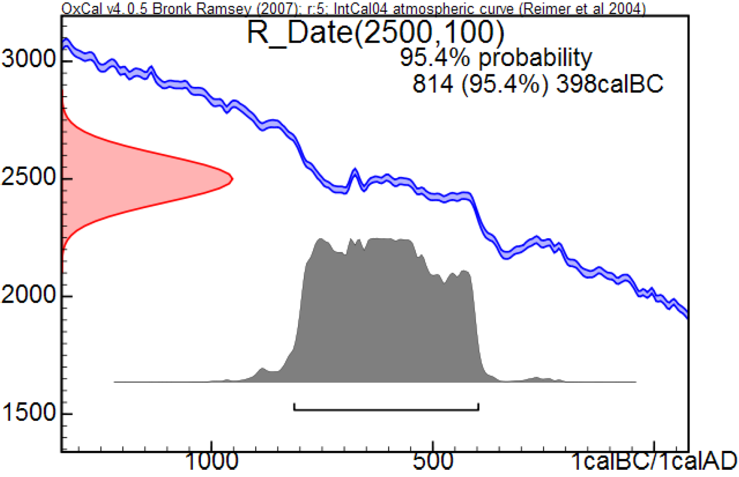
Fig. 1: Example OxCal calibration (from Fig.1 of Keenan, 2012, Calibration of a radiocarbon age)
Figure 1, from Fig. 1 in Doug’s paper, shows an example of an OxCal calibration, with the resulting 95.4% (±2 sigma for a Gaussian distribution) probability range marked by the thin bar above the x-axis. The red curve on the y-axis is centred on the 14C age derived by measurement (the radiocarbon or 14C determination) and shows the likelihood for that determination as a function of true 14C age. The likelihood for a 14C determination is the relative probability, for any given true 14C age, of having obtained that determination given the uncertainty in 14C determinations. The blue calibration curve shows the relationship between true 14C age (on the y-axis) and true calendar age on the x-axis. Its vertical width represents calibration uncertainty. The estimated PDF for calendar age is shown in grey. Ignoring the small effect of the calibration uncertainty, the PDF simply expresses the 14C determination’s likelihood as a function of calendar age. It represents both the likelihood function for the determination and – since a uniform prior for calendar age is used – the posterior PDF for the true calendar age (Bayes’ theorem giving the posterior as the normalised product of the prior and the likelihood function).
By contrast to OxCal’s subjective Bayesian, uniform prior based method, an objective Bayesian approach would involve computing a noninformative prior for ti. The standard choice would normally be Jeffreys’ prior. Doing so is somewhat problematic here in view of the calibration curve not being monotonic – it contains reversals – and also having varying uncertainty.
If the calibration curve were monotonic and had an unvarying error magnitude, the calibration curve error could be absorbed into a slightly increased 14C determination error, as both these uncertainty distributions are assumed Gaussian. Since the calibration curve error appears small in relation to 14C determination error, and typically only modestly varying over the 14C determination error range, I will make the simplifying assumption that it can be absorbed into an increased 14C determination error. The statistical relationship then becomes, given independence of calibration curve and radiocarbon determination uncertainty:
d14C ~ N( c(ti), sqrt(σc²+σd²) ) (3)
On that basis, and ignoring also the calibration curve being limited in range, it follows that Jeffreys’ prior for ti would equal the absolute derivative (slope) of calibrated 14C age with respect to calendar date. Moreover, in the absence of non-monotonicity it is known that in a case like this the Jeffreys’ prior is completely noninformative. Jeffreys’ prior would in fact provide exact probability matching – perfect agreement between the objective Bayesian posterior cumulative distribution functions (CDFs – the integrals of PDFs) and the results of repeated testing. The reason for the form here of Jeffreys’ prior is fairly clear – where the calibration curve is steep and hence its derivative with respect to calendar age is large, the error probability (red shaded area) between two nearby values of t14C corresponds to a much smaller ti range than when the derivative is small.
An alternative way of seeing that a noninformative prior for calendar age should be proportional to the derivative of the calibration curve is as follows. One can perform the Bayesian inference step to derive a posterior PDF for the true 14C age, t14C, using a uniform prior for 14C age – which as stated previously is, given the assumed Gaussian error distribution, noninformative. That results in a posterior PDF for 14C age that is identical, up to proportionality, to its likelihood function. Then one can carry out a change of variable from t14C to ti. The standard (Jacobian determinant) formula for converting a PDF between two variables, where one is a function of the other, involves multiplying the PDF, expressed in terms of the new variable, by the absolute derivative of the inverse transformation – the derivative of t14C with respect to ti. Taking this route, the objective posterior PDF for calendar age is the normalised product of the 14C age likelihood function (since the 14C objective Bayesian posterior is proportional to its likelihood function), expressed in terms of calendar age, multiplied by the derivative of t14C with respect to ti. That is identical, as it should be, to the result of direct objective Bayesian inference of calendar age using the Jeffreys’ prior.
3. Examining various methods using a simple stylised calibration curve
In order to make the problem analytically tractable and the performance of different methods – in terms of probability matching – easily testable, I have created a stylised calibration curve. It consists of the sum of three scaled shifted sigmoid functions. The curve exhibits both plateaus and steep regions whilst being smooth and monotonic and having a simple derivative.
Figure 2 shows similar information to Figure 1 but with my stylised calibration curve instead of a real one. The grey wings of the curve represent a fixed calibration curve error, which, as discussed, I absorb into the 14C determination error. The pink curve, showing the Bayesian posterior PDF using a uniform prior in calendar age, corresponds to the grey curve in Figure 1. It is highest over the right hand plateau, which corresponds to the centre of the red radiocarbon age error distribution, but has a non-negligible value over the left hand plateau as well. The figure also shows the objective Jeffreys’ prior (dotted green line), which reflects the derivative of the calibration curve. The objective Bayesian posterior using that prior is shown as the solid green line. As can be seen, it is very different from the uniform-calendar-year-prior based posterior that would be produced by the OxCal or Calib programs for this 14C determination (if they used this calibration curve).
 Fig. 2: Bayesian inference using uniform and objective priors with a stylised calibration curve
The Jeffreys’ prior (dotted green line) has bumps wherever the calibration curve has a high slope, and is very low in plateau regions. Subjective Bayesians will probably throw up their hands in horror at it, since it would be unphysical to think that the probability of a sample having any particular calendar age depended on the shape of the calibration curve. But that is to mistake the nature of a noninformative prior, here Jeffreys’ prior. A noninformative prior has no direct probabilistic interpretation. As a standard textbook (Bernardo and Smith, 1994) puts it in relation to reference analysis, arguably the most successful approach to objective Bayesian inference: “The positive functions π(θ) [the noninformative reference priors] are merely pragmatically convenient tools for the derivation of reference posterior distributions via Bayes’ theorem”.
Rather than representing a probabilistic description of existing evidence as to a probability distribution for the parameter being estimated, a noninformative prior primarily reflects (at least in straightforward cases) how informative, at differing values of the parameter, the data is expected to be about the parameter. That in turn reflects how precise the data are in the relevant region and how fast expected data values change with the parameter value. This comes back to the relationship between distances in parameter space and distances in data space that I mentioned earlier.
It may be thought that the objective posterior PDF has an artificial shape, with peaks and low regions determined, via the prior, by the vagaries of the calibration curve and not by genuine information as to the true calendar age of the sample. But one shouldn’t pay too much attention to PDF shapes; they can be misleading. What is most important in my view is the calendar age ranges the PDF provides, which for one-sided ranges follow directly from percentage points of the posterior CDF.
By a one-sided x% range I mean the range from the lowest possible value of the parameter (here, zero) to the value, y, at which the range is stated to contain x% of the posterior probability. An x1–x2% range or interval for the parameter is then y1 − y2, where y1 and y2 are the (tops of the) one-sided x1% and x2% ranges. Technically, this is a credible interval, as it relates to Bayesian posterior probability.
By contrast, a (frequentist) x% one-sided confidence interval with a limit of y can, if accurate, be thought of as one calculated to result in values of y such that, upon indefinitely repeated random sampling from the uncertainty distributions involved, the true parameter value will lie below y in x% of cases. By definition, an accurate confidence interval exhibits perfect frequentist coverage and so represents, for an x% interval, exact probability matching. If one-sided Bayesian credible intervals derived using a particular prior pass that test then they and the prior used are said to be probability matching. In general, Bayesian posteriors cannot be perfectly probability matching. But the simplified case presented here falls within an exception to that rule, and use of Jeffreys’ prior should in principle lead to exact probability matching.
The two posterior PDFs in Figure 2 imply very different calendar age uncertainty ranges. As OxCal reports a 95.4% range, I’ll start with the 95.4% ranges lying between the 2.3% and 97.7% points of each posterior CDF. Using a uniform prior, that range is 365–1567 years. Using Jeffreys’ prior, the objective Bayesian 2.3–97.7% range is 320–1636 years – somewhat wider. But for a 5–95% range, the difference is large: 395–1472 years using a uniform prior versus 333–1043 years using Jeffreys’ prior.
Note that OxCal would report a 95.4% highest posterior density (HPD) range rather than a range lying between the 2.3% and 97.7% points the posterior CDF. A 95.4% HPD range is one spanning the region with the highest posterior densities that includes 0.954 probability in total; it is necessarily the narrowest such range. HPD ranges are located differently from those with equal probability in both tails of a probability distribution; they are narrower but not necessarily better.
What about confidence intervals, a non-Bayesian statistician would rightly ask? The obvious way of obtaining confidence intervals is to use likelihood-based inference, specifically the signed root log-likelihood ratio (SRLR). In general, the SRLR only provides approximate confidence intervals. But where, as here, the parameter involved is a monotonic transform of a variable with a Gaussian distribution, SRLR confidence intervals are exact. So what are the 2.3–97.7% and 5–95% SRLR-derived confidence intervals? They are respectively 320–1636 years and 333–1043 years – identical to the objective Bayesian ranges using Jeffreys’ prior, but quite different from those using a uniform prior. I would argue that the coincidence of the Jeffreys’ prior derived objective Bayesian credible intervals and the SRLR confidence intervals reflects the fact that here both methods provide exact probability matching.
4. Numerical testing of different methods using the stylised calibration curve
Whilst an example is illuminating, in order properly to compare the performance of the different methods one needs to carry out repeated testing of probability matching based on a large number of samples: frequentist coverage testing. Although some Bayesians reject such testing, most people (including most statisticians) want a statistical inference method to produce, over the long run, results that accord with relative frequencies of outcomes from repeated tests involving random draws from the relevant probability distributions. By drawing samples from the same uniform calendar age distribution on which Bronk Ramsey’s method is predicated, we can test how well each method meets that aim. This is a standard way of testing statistical inference methods. Clearly, one wants a method also to produce accurate results for samples that – unbeknownst to the experimenter – are drawn from individual regions of the age range, and not just for samples that have an equal probability of having come from any year throughout the entire range.
I have accordingly carried out frequentist coverage testing, using 10,000 samples drawn at random uniformly from both the full extent of my calibration curve and from various sub-regions of it. For each sampled true calendar age, a 14C determination age is sampled randomly from a Gaussian error distribution. I’ve assumed an error standard deviation of 30 14C years, to include calibration curve uncertainty as well as that in the 14C determination. Whilst in principle I should have used somewhat different illustrative standard deviations for different regions, doing so would not affect the qualitative findings.
In these frequentist coverage tests, for each integral percentage point of probability the proportion of cases where the true calendar age of the sample falls below the upper limit given by the method involved for a one-sided interval extending to that percentage point is computed. The resulting proportions are then plotted against the percentage points they relate to. Perfect probability matching will result in a straight line going from (0%, 0) to (100%,1). I test both subjective and objective Bayesian methods, using for calendar age respectively a uniform prior and Jeffreys’ prior. I also test the signed root log-likelihood ratio method.
For the Bayesian method using a uniform prior, I also test the coverage of the HPD regions that OxCal reports. As HPD regions are two-sided, I compute the proportion of cases in which the true calendar age falls within the calculated HPD region for each integral percentage HPD region. Since usually only ranges that contain a majority of the estimated posterior probability are of interest, only the right hand half of the HPD curves (HPD ranges exceeding 50%) is of practical significance. Note that the title and y-axis label in the frequentist coverage test figures refer to one-sided regions and should in relation to HPD regions be interpreted in accordance with the foregoing explanation.
I’ll start with the entire range, except that I don’t sample from the 100 years at each end of the calibration curve. That is because otherwise a significant proportion of samples result in non-negligible likelihood falling outside the limits of the calibration curve. Figure 3 accordingly shows probability matching with true calendar ages drawn uniformly from years 100–1900. The results are shown for four methods. The first two are subjective Bayesian using a uniform prior as per Bronk Ramsey – from percentage points of the posterior CDF and from highest posterior density regions. The third is objective Bayesian employing Jeffreys’ prior, from percentage points of the posterior CDF. The fourth uses the non-Bayesian signed root log-likelihood ratio (SRLR) method. In this case, all four methods give good probability matching – their curves lie very close to the dotted black straight line that represents perfect matching.
 Fig. 3: Probability matching from frequentist coverage testing with calendar ages of 100–1900 years
Now let’s look at sub-periods of the full 100–1900 year period. I’ve picked periods representing both ranges over which the calibration curve is mainly flattish and those where it is mainly steep. I start with years 100–500, over most of which the calibration curve is steep. The results are shown in Figure 4. Over this period, SRLR gives essentially perfect matching, while the Bayesian methods give mixed results. Jeffreys’ prior gives very good matching – not quite perfect, probably because for some samples there is non-negligible likelihood at year zero. However, posterior CDF points using a uniform prior don’t provide very good matching, particularly for small values of the CDF (corresponding to the lower bound of two-sided uncertainty ranges). Posterior HPD regions provide rather better, but still noticeably imperfect, matching.
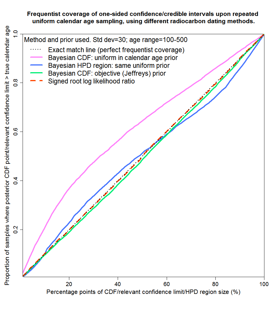 Fig. 4: Probability matching from frequentist coverage testing with calendar ages of 100–500 years
Figure 5 shows results for the 500–1000 range, which is flat except near 1000 years. The conclusions are much as for 100–500 years save that Jeffreys’ prior now gives perfect matching and that mismatching from posterior CDF points resulting from a uniform prior give smaller errors (and in the opposite direction) than for 100–500 years.
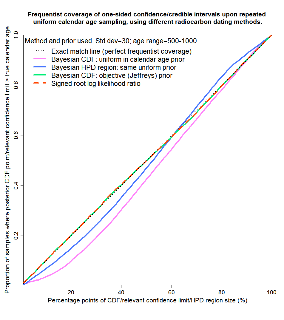 Fig. 5: Probability matching from frequentist coverage testing with calendar ages of 500–1000 years
Now we’ll take the 1000–1100 years range, which asymmetrically covers a steep region in between two plateaus of the calibration curve. As Figure 6 shows, this really separates the sheep from the goats. The SRLR and objective Bayesian methods continue to provide virtually perfect probability matching. But the mismatching from the posterior CDF points resulting from a uniform prior Bayesian method is truly dreadful, as is that from HPD regions derived using that method. The true calendar age would only lie inside a reported 90% HPD region for some 75% of samples. And over 50% of samples would fall below the bottom of a 10–90% credible region given by the posterior CDF points using a uniform prior. Not a very credible region at all.
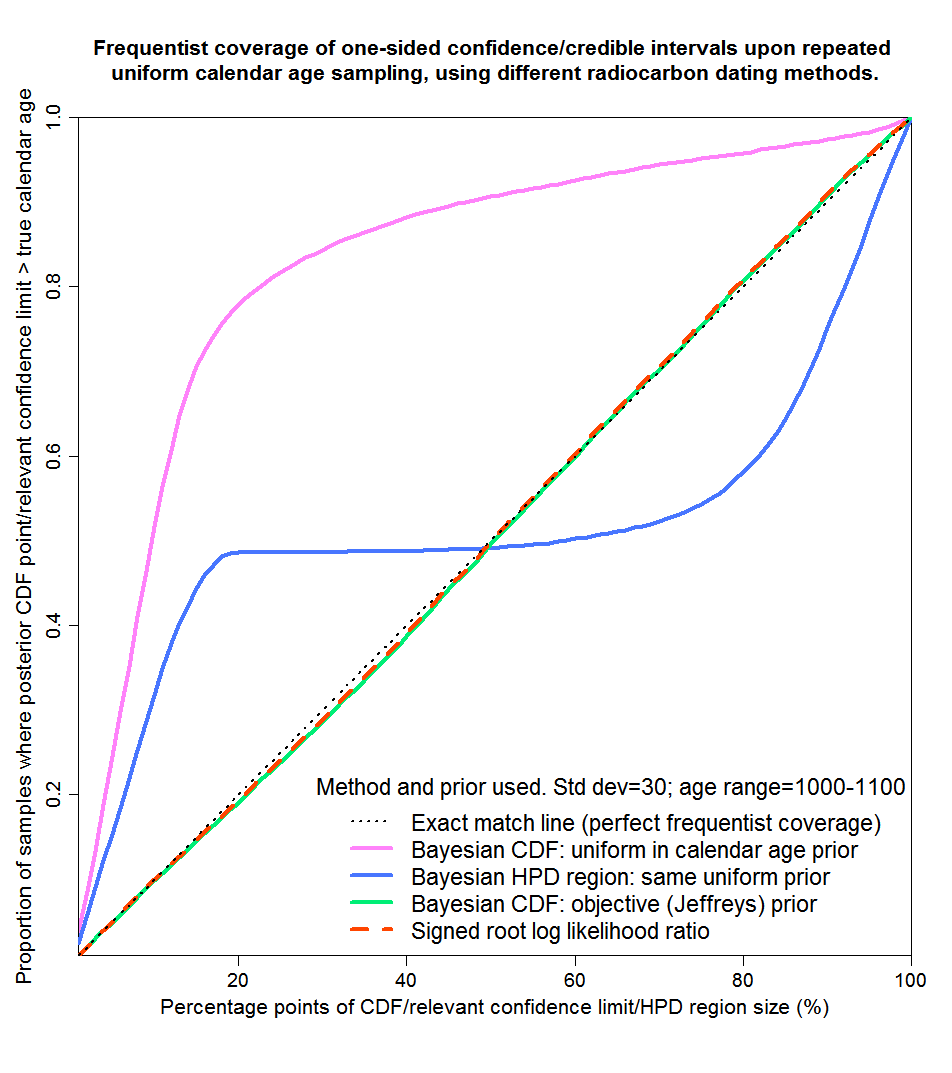 Fig. 6: Probability matching from frequentist coverage testing with calendar ages of 1000–1100 years
Figure 7 shows that for the next range, 1100–1500 years, where the calibration curve is largely flat, the SRLR and objective Bayesian methods again provide virtually perfect probability matching. However, the uniform prior Bayesian method again fails to provide reasonable probability matching, although not as spectacularly badly as over 1000–1100 years. In this case, symmetrical credible regions derived from posterior CDF percentage points, and HPD regions of over 50% in size, will generally contain a significantly higher proportion of the samples than the stated probability level of the region – the regions will be unnecessarily wide.
 Fig. 7: Probability matching from frequentist coverage testing with calendar ages of 1100–1500 years
Finally, Figure 8 shows probability matching for the mainly steep 1500–1900 years range. Results are similar to those for years 100–500, although the uniform prior Bayesian method gives rather worse matching than it does for years 100–500. Using a uniform prior, the true calendar age lies outside the HPD region noticeably more often than it should, and lies beyond the top of credible regions derived from the posterior CDF twice as often as it should.
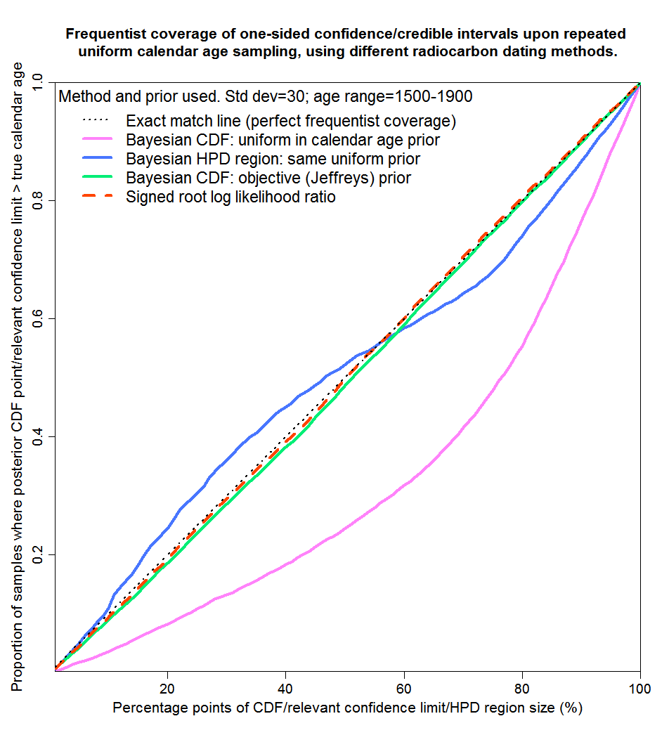
Fig. 8: Probability matching from frequentist coverage testing with calendar ages of 1500–1900 years
5. Discussion and Conclusions
The results of the testing are pretty clear. In whatever range the true calendar age of the sample lies, both the objective Bayesian method using a noninformative Jeffreys’ prior and the non-Bayesian SRLR method provide excellent probability matching – almost perfect frequentist coverage. Both variants of the subjective Bayesian method using a uniform prior are unreliable. The HPD regions that OxCal provides give less poor coverage than two-sided credible intervals derived from percentage points of the uniform prior posterior CDF, but at the expense of not giving any information as to how the missing probability is divided between the regions above and below the HPD region. For both variants of the uniform prior subjective Bayesian method, probability matching is nothing like exact except in the unrealistic case where the sample is drawn equally from the entire calibration range – in which case over-coverage errors in some regions on average cancel out with under-coverage errors in other regions, probably reflecting the near symmetrical form of the stylised overall calibration curve.
I have repeated the above tests using 14C error standard deviations of 10 years and 60 years instead of 30 years. Results are qualitatively the same.
Although I think my stylised calibration curve captures the essence of the principal statistical problem affecting radiocarbon calibration, unlike real 14C calibration curves it is monotonic. It also doesn’t exhibit variation of calibration error with age, but such variation shouldn’t have a significant impact unless, over the range where the likelihood function for the sample is significant, it is substantial in relation to 14C determination error. Non-monotonicity is more of an issue, and could lead to noticeable differences between inference from an objective Bayesian method using Jeffreys’ prior and from the SRLR method. If so, I think the SRLR results are probably to be preferred, where it gives a unique contiguous confidence interval. Jeffreys’ prior, which in effect converts length elements in 14C space to length elements in calendar age space, may convert single length elements in 14C space to multiple length elements in calendar age space when the same 14C age corresponds to multiple calendar ages, thus over-representing in the posterior distribution the affected parts of the 14C error distribution probability. Initially I was concerned that the non-monotonicity problem was exacerbated by the existence of calibration curve error, which results in uncertainty in the derivative of 14C age with respect to calendar age and hence in Jeffreys’ prior. However, I now don’t think that is the case.
Does the foregoing mean the SRLR method is better than an objective Bayesian method? In this case, perhaps, although the standard form of SRLR isn’t suited to badly non-monotonic parameter–data relationships and non-contiguous uncertainty ranges. More generally, the SRLR method provides less accurate probability matching when error distributions are neither normal nor a transforms of a normal.
Many people may be surprised that the actual probability distribution of the calendar date of samples for which radiocarbon determinations are carried out is of no relevance to the choice of a prior that leads to accurate uncertainty ranges and hence is, IMO, appropriate for scientific inference. Certainly most climate scientists don’t seem to understand the corresponding point in relation to climate sensitivity. The key point here is that the objective Bayesian and the SRLR methods both provide exact probability matching whatever the true calendar date of the sample is (provided it is not near the end of the calibration curve). Since they provide exact probability matching for each individual calendar date, they are bound to provide exact probability matching whatever probability distribution for calendar date is assumed by the drawing of samples.
How do the SRLR and objective Bayesian methods provide exact probability matching for each individual calendar date? It is easier to see that for the SRLR method. Suppose samples having the same fixed calendar date are repeatedly drawn from the radiocarbon and calibration uncertainty distributions. The radiocarbon determination will be more than two standard deviations (of the combined radiocarbon and calibration uncertainty level) below the exact calibration curve value for the true calendar date in 2.3% of samples. The SRLR method sets its 97.7% bound at two standard deviations above the radiocarbon determination, using the exact calibration curve to convert this to a calendar date. That bound must necessarily lie at or above the calibration curve value for the true calendar date in 97.7% of samples. Ignoring non-monotonicity, it follows that the true calendar date will not exceed the upper bound in 97.7% of cases. The bound is, given the statistical model, an exact confidence limit by construction. Essentially Jeffreys’ prior achieves the same result in the objective Bayesian case, but through operating on probability density rather than on its integral, cumulative probability.
Bayesian methods also have the advantage that they can naturally incorporate existing information about parameter values. That might arise where, for instance, a non-radiocarbon based dating method had already been used to estimate a posterior PDF for the calendar age of a sample. But even assuming there is genuine and objective probabilistic prior information as to the true calendar year, what the textbooks tell one to do may not be correct. Suppose the form of the data–parameter relationship differs between the existing and new information, and it is wished to use Bayes’ theorem to update, using the likelihood from the new radiocarbon measurement, a posterior PDF that correctly reflects the existing information. Then simply using that existing posterior PDF as the prior and applying Bayes’ theorem in the standard way will not give an objective posterior probability density for the true calendar year that correctly combines the information in the new measurement with that in the original posterior PDF. It is necessary to use instead a modified form of Bayesian updating (details of which are set out in my paper at http://arxiv.org/abs/1308.2791). It follows that it the existing information is simply that the sample must have originated between two known calendar dates, with no previous information as to how likely it was to have come from any part of the period those dates define, then just using a uniform prior set to zero outside that period would bias estimation and be unscientific.
And how does Doug Keenan’s ‘discrete’ calibration method fit in to all this? So far as I can see, the uncertainty ranges it provides will be considerably closer to those derived using objective Bayesian or SRLR methods than to those given by the OxCal and Calib methods, even though like them it uses Bayes’ theorem with a uniform prior. That is because, like the SRLR and (given monotonicity) Jeffreys’ prior based objective Bayesian methods, Doug’s method correctly converts, so far as radiocarbon determination error goes, between probability in 14C space and probability in calendar year space. I think Doug’s treatment of calibration curve error avoids, through renormalisation, the multiple counting of 14C error probability that may affect a Jeffreys’ prior based objective Bayesian method when the calibration curve is non-monotonic. However, I’m not convinced that his treatment of calibration curve uncertainty is noninformative even in the absence of it varying with calendar age. Whether that makes much difference in practice, given that 14C determinant error appears normally to be the larger of the two uncertainties by some way, is unclear to me.
Does the uniform prior subjective Bayesian method nevertheless have advantages? Probably. It may cope with monotonicity better than the basic objective Bayesian method I have set out, particularly where that leads to non-contiguous uncertainty ranges. It may also make it simpler to take advantage of chronological information where there is more than one sample. And maybe in many applications it is felt more important to have realistic looking posterior PDFs than uncertainty ranges that accurately reflect how likely the true calendar date is to lie within them.
I can’t help wondering whether it might help if people concentrated on putting interpretations on CDFs rather than PDFs. Might it be better to display the likelihood function from a radiocarbon determination (which would be identical to the subjective Bayesian posterior PDF based on a uniform prior) instead of a posterior PDF, and just to use an objective Bayesian PDF (or the SRLR) to derive the uncertainty ranges? That way one would both get a realistic picture of what calendar age ranges were supported by the data, and a range that the true age did lie above or below in the stated percentage of instances.
Professor Bronk Ramsey considers that knowledge of the radiocarbon calibration curve does give us quantitative information on the prior for 14C ‘age’. He argues that the belief that in reality calendar dates of samples are spread uniformly means that a non-uniform prior in 14C age is both to be expected and is what you would want. That would be fine if the prior assumption made about calendar dates actually conveyed useful information.
Where genuine prior information exists, one can suppose that it is equivalent to a notional observation with a certain probability density, from which a posterior density of the parameter given that observationhas been calculated using Bayes’ theorem with a noninformative ‘pre-prior’, with the thus computed posterior density being employed as the prior density (Hartigan, 1965).
However, a uniform prior over the whole real line conveys no information. Under Hartigan’s formulation, it’s notional observation has a flat likelihood function and a flat pre-prior. Suppose the transformation from calendar date to 14C age using the calibration curve is effected before the application of Bayes’ theorem to the notional observation for a uniform prior. Then its likelihood function remains flat – what becomes non-uniform is the pre-prior. The corresponding actual prior (likelihood function for notional observation multiplied by the pre-prior) in 14C age space is therefore nonlinear, as claimed. But when the modified form of Bayesian updating set out in my arXiv paper is applied, that prior has no influence on the shape of the resulting posterior PDF for true 14C age and nor, therefore, for the posterior for calendar date. In order to affect an objective Bayesian posterior, one has to put some actual prior information in. For instance, that could be in the form of a Gaussian distribution for calendar date. In practice, it may be more realistic to do so for the relationship between the calendar dates of two samples, perhaps based on their physical separation, than for single samples.
Let me give a hypothetical non-radiocarbon example that throws light on the uniform prior issue. Suppose that a satellite has fallen to Earth and the aim is to recover the one part that will have survived atmospheric re-entry. It is known that it will lie within a 100 km wide strip around the Earth’s circumference, but there is no reason to think it more likely to lie in any part of that strip than another, apart from evidence from one sighting from space. Unfortunately, that sighting is not very precise, and the measurement it provides (with Gaussian error) is non-linearly related to distance on the ground. Worse, although the sighting makes clear which side of the Earth the satellite part has hit, the measurement is aliased and sightings in two different areas of the visible side cannot be distinguished. The situation is illustrated probabilistically in Figure 9.
 Fig. 9: Satellite part location problem
In Figure 9, the measurement error distribution is symmetrically bimodal, reflecting the aliasing. Suppose one uses a uniform prior for the parameter, here ground distance across the side of the Earth visible when the sighting was made, on the basis that the item is as likely to have landed in any part of the 100 km wide strip as in any other. Then the posterior PDF will indicate an 0.825 probability that the item lies at a location below 900 (in the arbitrary units used). If one instead uses Jeffreys’ prior, the objective Bayesian posterior will indicate a 0.500 probability that it does so. If you had to bet on whether the item was eventually found (assume that it is found) at a location below 900, what would you consider fair odds, and why?
Returning now to radiocarbon calibration, there seems to me no doubt that, whatever the most accurate method available is, Doug is right about a subjective Bayesian method using a uniform prior being problematical. By problematical, I mean that calibration ranges from OxCal, Calib and similar calibration software will be inaccurate, to an extent varying from case to case. Does that mean Bronk Ramsey is guilty of research misconduct? As I said initially, certainly not in my view. Subjective Bayesian methods are widely used and are regarded by many intelligent people, including statistically trained ones, as being theoretically justified. I think views on that will eventually change, and the shortcomings and limits of validity of subjective Bayesian methods will become recognised. We shall see. There are deep philosophical differences involved as to how to interpret probability. Subjective Bayesian posterior probability represents a personal degree of belief. Objective Bayesian posterior probability could be seen as, ideally, reflecting what the evidence obtained implies. It could be a long time before agreement is reached – there aren’t many areas of mathematics where the foundations and philosophical interpretation of the subject matter are still being argued over after a quarter of a millennium!
A PDF of this article and the R code used for the frequentist coverage testing are available at http://niclewis.files.wordpress.com/2014/04/radiocarbon-calibration-bayes.pdf and http://niclewis.files.wordpress.com/2014/04/radiocarbon-dating-code.doc
[i] A statistical model is still involved, but no information as to the value of the parameter being estimated is introduced as such. Only in certain cases is it possible to find a prior that has no influence whatsoever upon parameter estimation. In other cases what can be sought is a prior that has minimal effect, relative to the data, on the final inference (Bernardo and Smith, 1994, section 5.4).
[ii] I am advised by Professor Bronk Ramsey that the method was originally derived by the Groningen radiocarbon group, with other notable related subsequent statistical publications by Caitlin Buck and her group and Geoff Nicholls.


127 Comments
A butterfly flaps its statistical wing,
Shudders run through that whole history thing.
==========
Should that be ‘a degree of personal belief’>?
1. No. The calibration curve takes account of changes in 14C production rates due to varying solar and geomagnetic shielding.
2. Within each hemisphere – there is a separate calibration curve for the southern hemisphere that has an offset of ~40 years (due to increased exchange of CO2 with the ocean in the southern hemisphere. Within each hemisphere 14C is assumed to be well mixed. There probably are regional deviations, but they are likely be minor.
50,000 years.
For the Holocene (and slightly beyond) tree rings of known age (via dendrochronology) are radiocarbon dated. These data are used to calculate the radiocarbon calibration curve, which can be used to infer solar activity. But for radiocarbon dating it doesn’t matter what caused the concentration of 14C to vary.
Other materials eg corals and macrofossild in varved lakes are used for older dates because trees are not available.
Actually the calibration curve beyond the treering range (ca 12 000 BP) is very decidedly shaky. And the “raw” C14 dates themselves are best regarded as minimum ages beyond c. 35 000 rcy BP.
The problem with using corals, speleothems etc is that in contrast to trees these do not derive their carbon direct from the atmosphere, so it is necessary to correct for admixture of “old” carbon, an admixture that may well have varied widely over time.
There are a number of older pleistocene treering chronologies, but unfortunately they are all “floating” and so can’t be tied down to an absolute chronology.
NIc, thanks for this. In addition to the intrinsic interest of the problem, it’s an illuminating illustration of the technique.
The graphs make it much easier to understand for somebody like me who is not familiar with the lingo but has a basic understanding of probabilities. I don’t fully understand the mathematics behind it but overall the argument presented here is pretty convincing.
Nic
this was really helpful
“Rather than representing a probabilistic description of existing evidence as to a probability distribution for the parameter being estimated, a noninformative prior primarily reflects (at least in straightforward cases) how informative, at differing values of the parameter, the data is expected to be about the parameter. That in turn reflects how precise the data are in the relevant region and how fast expected data values change with the parameter value. This comes back to the relationship between distances in parameter space and distances in data space that I mentioned earlier.”
Very interesting and well explained.
You had me until you took shots at Bayesians.
You wrote: I think views on that will eventually change, and the shortcomings and limits of validity of subjective Bayesian methods will become recognised.
Well, sure. But, if you believed that a measured quantity should never be less than one, you would treat observations of 0.87 with suspicion. In practical terms, people are subjective Bayesians all the time. Richard Feynman said it well:
It is probably better to realize that the probability concept is in a sense subjective, that it is always based on uncertain knowledge, and that its quantitative evaluation is subject to change as we obtain more information.
He said that in 1962 when Bayesian reasoning was widely deprecated.
Now, some things that are done in the name of Bayes may be a little questionable.
Chuck
chuck
I have no problem with what Feynmann said. My objection is to when subjective Bayesians misuse the available information in estimating probability, so that the result does not fairly reflect the available information. There’s often no perfect answer, I realise.
Well,I’m against misuse of anything. But,it seems to me (a non-statistician) that frequentist theory is misused even more than Bayesian. Look at all the significance tests and tests of the null hypothesis done by climate scientists. You would think it is 1960!
I was first exposed to Bayesian reasoning in the context of decision theory. It seems to me incontrovertible that if you strongly believe that A is true but a few, unreliable measurements indicate that B is slightly more likely to be true, you should bet that A is true. Frequentist reasoning leads to the opposite conclusion.
But, as I said, I’m against misuse and all tools can be misused.
Again, you posting was excellent—it was clear and instructive. Don’t let my philosophical objection confuse my fundamental point.
Chuck
Chuck,
“…It seems to me incontrovertible that if you strongly believe that A is true but a few, unreliable measurements indicate that B is slightly more likely to be true, you should bet that A is true….”
The problem with this is the “belief” element. If the potential for A and B are both affected by the measurements of B, regardless of how unreliable measures of B might be, you simply don’t have enough information to make an informed decision. Both views should be stated and analyzed, and the need for better information highlighted. One point that underscores this is several recent metastudies that have pointed a pattern of earlier studies investigating a given hypothesis, particularly in medicine, that tend to be more confirmatory than follow up studies. That is, early studies tend look very positive, while support in later investigations tends to weaken. So, treating earlier studies as more indicative of reality – they are the prior information available – you would, if I followed your argument, find yourself betting against increasing odds of being wrong.
This article is an example of the reason I like reading when a mathematically sound person writes to convey information! I simply find it enjoyable and enlightning. Reminded me of the motivation/summary lecture prior to getting down to the nitty gritty of the mathematics proof.
But one question for Nic:
How far off is the normalized(f(x)) where f(x) = g(C(x)) where C is the calibration curve, g(y) is the pdf for the Radio Determined Age and then the normalized(f) is the pdf for the calendar age, as compared to the Bayesian Posterior using Uniform Prior?
timothy
If I understand your question correctly, they will be identical, since the [posterior] pdf for the 14C determined age is identical to its likelihood function (if one uses a uniform in 14C prior, which would be usual with a Gaussian error distribution).
To convert the posterior pdf g(y) for the 14C determined age into a pdf for calendar age one would need to multiply by the derivative of the inverse transform, so one would have:
f(x) = g(C(x)) dC(x)/dx
but I think the non-monotonicity of C(x) is a problem here.
Thanks for the post. I will have to read more slowly and inwardly digest – perhaps later over the weekend.
I should perhaps clarify that I wasn’t saying the OxCal method was necessarily right, only that it was the posterior you got from a uniform prior on calender year, which was what was being commonly assumed. I would tend to take such a report only as a ‘neutral’ way to express an experimental result before combining it with a more sensible prior on calender year based on other evidence. The idea is that it makes it easier for the result to be re-used by people with different priors, and makes it clear what part the radiocarbon evidence is contributing to the result versus any other evidence. I agree with Nic that assuming a uniform distribution as one’s actual prior is a risky operation.
I’m pretty sure that in any reasonable archaeological context you’re always going to have some prior information. Something found in a sealed Egyptian tomb is not equally likely to have been put there 40 years ago as 4000 years ago.
My view was that the meaning and proper interpretation of the OxCal result was poorly explained, and that they should have been able to answer Doug’s questions had they properly understood the method themselves. Doug’s confusion was understandable.
—
Nic’s post reminds me of the story I once heard about the man who lost his keys at night, and was walking from street light to street light, pausing at each to search in the patch of illumination. When asked why he was only looking under the street lights, surely he didn’t think the keys were any more likely to have fallen out there, he replied “Maybe not, but I think I’m more likely to find them there.”
“I’m pretty sure that in any reasonable archaeological context you’re always going to have some prior information. Something found in a sealed Egyptian tomb is not equally likely to have been put there 40 years ago as 4000 years ago.”
Some information yes, but you might be surprised by how often objects found in apparently undisturbed and sealed context turn out to be intrusive (mostly younger) when dated by C14 (or other method).
One of the loud archaeological debates concerns contamination of younger material by older carbon when the contamination is not due to a reservoir effect, e.g the debate over the early dates at Meadowcroft Rockshelter in Pennsylvania. In fact, to significantly increase the apparent age of a sample would necessitate significantly increasing the bulk of the sample with the contaminant. It is vastly simpler to contaminate a sample with younger material without detectably modifying the sample. The biggest hazard to a good date estimate is still the laboratory handling.
Steve M, Mosher, Dave
Thanks! BTW, it’s worth looking at my R code – there are a couple of useful stand-alone utilities included, in particular one that computes specified percentage points for multiple PDFs or CDFs (and from [profile] likelihoods) and can also add them to a graph as box plots.
Forgive me… (really, forgive me)… But when I saw this post and saw that you were authoring it, I was expecting some eventual prose directly engaging the latest response(criticism) to your recent paper:
http://www.realclimate.org/index.php/archives/2014/04/shindell-on-constraining-the-transient-climate-response/
I pretty-much tore through your words searching for the payoff and didn’t find it. Obviously it’s no matter, considering you’re free to write about whatever whenever 😉 …I just think there’s a couple people out there interested to hear if the case is closed there, or if there is still a matter of non-impassed debate regarding each other’s work.
I shall respond to Shindell, but I’ve had lots to do and Bayesian stats stuff also interests me. FWIW, I think the effect Shindell is making a noise about is likely very small in the real world.
As an initial move, I posted a comment on Troy Master’s blog (he also had a post attacking Shindell’s paper), in which I pointed out that Shindell’s RC piece, far from answering all the substantive points in my CA post, had simply ignored most of them. See http://troyca.wordpress.com/2014/03/15/does-the-shindell-2014-apparent-tcr-estimate-bias-apply-to-the-real-world/#comment-1427 .
Ah, I see it now.
Such is life in the blogosphere– it’s really hard to keep up with so many places where the things you’re looking for might be found.
A problem for all of us. Nic posted this in a comment on Bishop Hill ten days ago, which is how I knew to look in troyca’s direction:
Keep watching all these spaces 🙂
I’d like to take a minute to compliment you on the quality of your prose. It’s hard to write clearly about this and you did an excellent job.
Thanks, Tom!
Nic,
Thanks for the clearly written exposition of how a standard “subjective” Bayesian analysis can sometimes differ dramatically from an analysis based on an “objective” Bayesian prior (specifically, Jeffreys’ prior). As I’ll explain below, it illuminates very well the way in which your philosophical standpoint is not one I agree with.
However, I am in agreement regarding the technical details and calculations you give, with one exception – after showing that the subjective Bayesian credible interval based on the posterior CDF has perfect probability matching when the parameter value is randomly chosen from the subjective prior that is used, you remark that this is “probably reflecting the near symmetrical form of the stylised overall calibration curve”. Actually, it has nothing to do with that, and in fact you didn’t even need to run the program to find this out. One can easily prove theoretically that the probability that the credible interval based on the posterior CDF will contain the true parameter value will always be exactly as specified, if you average over true parameter values drawn from the prior used to construct the posterior. Subjective Bayesian procedures are always perfectly consistent on their own terms.
Given that, it’s easy to see why a subjective Bayesian method will usually NOT produce perfect probability matching when averaging over a distribution for true parameter values that is different from the prior it uses. In particular, if you draw true parameter values from a more restricted interval (or as an extreme, fix the true parameter to a single value), the subjective Bayesian method will think that some values are possible that in fact never occur, while thinking other values are less probable than they actually are (since with the range restricted, those values that remain possible occur more often). This is no surprise to subjective Bayesians, though the carbon-14 dating example illustrates it in particularly nice fashion.
That the “objective” Bayesian method using Jeffreys’ prior will produce perfect probability matching is most easily seen as being due to the general fact that an analysis using the Jeffreys’ prior is not affected by applying some monotonic transformation to the parameter (and then interpreting the results as transformed, of course). Standard frequentist tests of a null hypothesis based on a Gaussian observation are also unaffected by such a monotonic transformation. So in both cases, one can construct a confidence/credible interval for the carbon-14 age by well-known methods (that exhibit perfect probability matching), and then simply transform the endpoints of this interval to calendar years using the calibration curve (which I’ll assume is known exactly, since uncertainty in it doesn’t seem to really affect the argument). The result will also have perfect probability matching.
But it doesn’t follow that these intervals with perfect probability matching actually make any sense. As you seem to realize, the posterior probability density function obtained using Jeffreys’ prior is both bizarre and unbelievable. In particular, calendar ages where the calibration curve is almost flat have almost zero posterior probability density, even when they are entirely compatible with the observed data. The posterior probability that the true calendar age is in some interval over which the calibration curve is almost flat is also close to zero, so it’s not just a case of some funny problem with interpreting what a probability density is. There’s just no way this makes any sense – for instance, in your example of Fig. 2, it makes no sense to conclude that the calendar age has almost zero probability of being in the interval 750 to 850, when these calendar ages are amongst those that are MOST compatible with the data, and we are assuming that there is no specific prior knowledge that would eliminate years in this range. Similarly, it makes no sense to conclude that the interval from 1100 to 1400 has almost zero probability, even though these years produce a fit to the data that is only modestly worse than the years with highest likelihood.
Since the posterior distribution obtained using Jeffreys’ prior is unbelievable, it provides no reason to believe in the credible interval computed from this posterior distribution (ie, regardless of whether the credible region is actually good, the fact that it was obtained from this unbelievable posterior distribution is not a valid reason to think it is good).
The frequentist confidence interval (which contains all points not rejected by a null hypothesis test) will of course have the proper coverage probability. But this is of no interest, since nobody cares about this coverage property – some people they may THINK that they care, but they really only care about the result of surreptitiously swapping the order of conditioning, converting the confidence interval into a pseudo-Bayesian credible interval, since that’s what they need to actually DO anything with the interval (other than putting it in a paper to satisfy some ritualistic requirement). Interpreting confidence intervals in this swapped fashion is very common, and may cause little harm when available prior information is vague anyway, but for carbon-14 age, there is actually very strong prior information (if the calibration curve is highly non-linear).
So I don’t think there is any valid justification for using the confidence/credible intervals you produce. Now, one problem with discussing this is that no actual use for the intervals has been specified. It’s quite possible that such intervals don’t answer the question that needs answering anyway, and that instead what is needed is, say, the posterior probability that the calendar age is between 1100 and 1400 (with these endpoints having been pre-specified as the ones of interest). If this range happens to lie entirely within or entirely outside the credible interval you found, you get a rough answer of sorts, but in general you should just directly find the answer to your actual question. One advantage of Bayesian inference using a posterior distribution is the ease of answering all sorts of questions like this. But it doesn’t work if your posterior distribution is nonsensical, as is the case here if you use Jeffreys’ prior.
Your satellite example is of interest because for this example you have explicitly specified the question of interest – where should we start searching in order to recover the satellite with the least effort? (Eg, perhaps it’s enough to decide whether we should first look below position 900, or above, as you mention.) You have also clearly indicated that the prior knowledge of the satellite’s location is uniform over the strip. And though you don’t specify the measurement process in detail, you’re also clearly assuming that its properties are known, and the actual measurement gives the likelihood function you plot.
With these assumptions, there is no doubt that the correct method is found by computing posterior probabilities based on the “subjective” uniform prior. It is NOT correct to use Jeffreys’ prior. This is just a mathematical fact. Subjective Bayesian inference is completely consistent within its own world, and given all your assumptions, that is the world we are dealing with. You will find this if you run simulations of satellites falling at positions uniformly distributed on the strip, sightings occurring with some measurement process such as you describe, inferences being done using the uniform prior and the Jeffreys’ prior, and people placing bets on the basis of one inference or the other. The bets based on Jeffreys’ prior will not win as much money on average as those based on the “subjective” uniform prior.
Now, in real problems, the issues are seldom so clear. For carbon-14 dating, it may be that posterior probabilities of any sort are not what is needed. The sample is probably being dated as part of some wider research project, and what is needed in the wider context may simply be the likelihood as a function of calendar year, with no need to combine this with any prior – instead, it will contribute one factor to the likelihood function of some grander model. Of course, if you know the posterior density based on a uniform prior, that immediately tells you the likelihood function too, so the distinction may be a bit academic.
For other problems (but not the carbon-14 dating problem as you’ve described it), issues arise with “nuisance parameters”, that affect the distribution of the data, but aren’t of direct interest. If there are lots of these, it becomes infeasible to just report the likelihood function, and the prior for the nuisance parameters can affect the posterior for the parameter of interest. I think statisticians working on “objective” or “reference” priors are probably mostly motivated by issues of this sort. For the problems in your post, however, there are no nuisance parameters, so this motive for using an “objective” prior is absent.
More generally, going beyond carbon-14 dating, you should note that using uniform priors is certainly not general practice for subjective Bayesians. In fact, most subjective Bayesians would never use a uniform prior for an unbounded quantity, since this does not correspond to any actual, proper probability distribution. (An exception would be when it’s clear that the prior has little influence anyway, and it’s just easier to use a uniform prior.)
The cardinal rule for Bayesian inference is DON’T IGNORE INFORMATION. This is obvious for data – if you’ve collected 1000 data points, it’s not valid to pick out 300 of them and report a posterior distribution that ignores the other 700. But it’s also true for prior information. For instance, a posterior distribution based on a uniform prior for an unbounded positive quantity is not valid when (as is always the case) you have reason to think that, past a certain point, large values of the parameter are highly implausible. Criticism of priors used in a subjective Bayesian analysis is entirely appropriate, but blindly using Jeffreys’ prior is not.
Radford Neal
Radford,
Thanks for commenting in detail. I think the fundamental difference between us is that you assume that genuine prior information exists as to the true calendar age of a sample, whereas I do not. I agree that, if genuine prior information does exist, then Jeffreys’ prior may not be the best choice. But your statement: “Given that, it’s easy to see why a subjective Bayesian method will usually NOT produce perfect probability matching when averaging over a distribution for true parameter values that is different from the prior it uses” reveals a major problem. In general, one doesn’t know what the distribution for true parameter values is.
Bronk Ramsey’s 2009 paper refers to the argument that “we should not include anything but the dating information and so the prior [for calendar age] becomes a constant”. It states that they normally do so iff there is a single event, setting p(tᵢ) ~ U( ∞,∞). To me, those statements show an intention for the uniform prior to represent ignorance, not a justified belief that the sample was in fact generated by a process that resulted in it having equal probability of it having originated in any calendar year and/or falling within a particular date range. And from a physical point of view, there could well be other probability distributions that are more plausible, such as exponential.
A method that only provides reliable uncertainty ranges if the sample was generated by a process that produces a distribution of sample ages matching as to both shape and extent the prior distribution used seems pretty unsatisfactory to me. By contrast, both an objective Bayesian method using Jeffreys’ prior and the SRLR method will provide exact probability matching whatever distribution of sample ages the process that actually generated the sample produces.
We agree that the posterior PDF produced by use of Jeffreys’ prior may look artificial. But I don’t agree with you that means one shouldn’t believe in credible intervals computed from such a posterior distribution. IMO, the probability matching properties of such credible intervals make them perfectly believable. Much more believable than credible intervals resulting from use of a subjective prior, when one doesn’t have any good reason to think that prior accurately reflects genuine prior information.
As I wrote, I think it may be more helpful here to report the likelihood function and to think of the posterior PDF as a way of generating a CDF and hence credible intervals rather than being useful in itself. I agree that realistic posterior PDFs can be very useful, but if the available information does not enable generation of a believable posterior PDF then why should it be right to invent one?
As you say, we don’t have the problem of nuisance parameters here, but I don’t see that as a reason against using noninformative prior where there is no genuine prior information.
You didn’t interpret my satellite example in the way I envisaged, no doubt because I didn’t express it very well and also because of its physical characteristics. My words “but there is no reason to think it more likely to lie in any part of that strip than another” were intended to indicate total ignorance, not that prior knowledge of the satellite’s location was equivalent to a uniform distribution over the strip. There is a difference. You are assuming it is known that the process which generated the impact location results in it being equally likely to lie in any part of the strip, so that there is genuine prior information. Whilst that is physically plausible, it was not specified. If you do make that assumption, then I agree with your analysis.
I agree with your point about not ignoring information. I have another cardinal rule: DON’T INVENT INFORMATION.
Nic: … you assume that genuine prior information exists as to the true calendar age of a sample, whereas I do not.
Well, subjective Bayesians think that there is always prior information. I do have my doubts about this in extreme cases like assigning prior probabilities to different cosmological theories, where it’s hard to see why people should have evolved to have intuitive knowledge of what’s plausible, but we’re not dealing with that sort of problem here. People have all sorts of information about what are more or less plausible dates for old pieces of parchment, tree stumps, or whatever. It’s unlikely that this will lead to a uniform prior, however, which is why I suspect that people are using that prior just as a way of communicating the likelihood function (while possibly being a bit confused about what they’re really doing).
Nic: We agree that the posterior PDF produced by use of Jeffreys’ prior may look artificial.
The posterior PDF produced by use of Jeffreys’ prior doesn’t just look “artificial”. It looks completely wrong. I think this is the most crucial point. Your example isn’t one that should convince readers to use Jeffreys’ prior because it gives exact probabililty matching for credible intervals. It’s an example that should convince readers that Jeffreys’ prior is flawed, and probability matching is not something one should insist on. Could there possibly be a clearer violation of the rule “DON’T INVENT INFORMATION”? The prior gives virtually zero probability to large intervals of calendar age based solely on the shape of the calibration curve, with this curve being the result of physical processes that almost certainly have nothing to do with the age of the sample.
Statistical inference procedures are ultimately justified as mathematical and computational formalizations of common sense reasoning. We use them because unaided common sense tends to make errors, or have difficulty in processing large amounts of information, just as we use formal methods for doing arithmetic because guessing numbers by eye or counting on our fingers is error prone, and is anyway infeasible for large numbers. So the ultimate way of judging the validity of statistical methods is to apply them in relatively simple contexts (such as this) and check whether the results stand up to well-considered common sense scrutiny. In this example, Jeffreys’ prior fails this test spectacularly.
I think you would maybe agree that Jeffreys’ prior is not to be taken seriously, given that you say the following:
Nic: … think of the posterior PDF as a way of generating a CDF and hence credible intervals rather than being useful in itself. I agree that realistic posterior PDFs can be very useful, but if the available information does not enable generation of a believable posterior PDF then why should it be right to invent one?
But with this comment, you seem to have adopted a strange position that may be unique to you. Frequentists usually don’t have much use for a posterior PDF for any purpose. And I think “objective” Bayesians aim to produce a posterior PDF that is sensible. I’m puzzled why you would bother to produce a posterior that you don’t believe is even close to being a proper expression of posterior belief, and then use it as a justification for the credible intervals that can be derived from it. If these credible intervals have any justification, it can’t be that. And in fact, for this example, you can (and do) justify these intervals as being confidence intervals according to standard frequentist arguments (albeit ones that I think are flawed in this context). So what is the point of the whole objective Bayesian argument?
Nic: My words “but there is no reason to think it more likely to lie in any part of that strip than another” were intended to indicate total ignorance, not that prior knowledge of the satellite’s location was equivalent to a uniform distribution over the strip. There is a difference. You are assuming it is known that the process which generated the impact location results in it being equally likely to lie in any part of the strip…
I think it is impossible to maintain this distinction between a physical random process and “ignorance”, which you don’t seem willing to represent using probability (even though that’s central to all Bayesian methods, subjective or not). Archetypal random processes such as coin flips are probably not actually random, in the sense of quantum uncertainty or thermal noise, but appear random only because of our ignorance of initial conditions, which could be eliminated by suitable measuring instruments (that are not impossible according to the laws of physics).
Among both frequentists and objective Bayesians, I think there is a degree of wishful thinking from wanting to find a procedure that avoids all “subjectivity”. But it’s just not possible. Refusal to admit that it’s not possible inevitably leads to methods that produce strange results.
Radford Neal:
The criterion should not be whether the results look wrong, but whether the method (including the implicit prior) looks wrong. The Jeffreys prior on C14 age should be rejected because it implies a bizarre prior on the calibrated date of interest, given the objective information in the calibration curve. This is why it gives bizarre posteriors sometimes, but we should not reject the results just because the posterior is subjectively “wrong”.
Hu,
Certainly, when judging whether a method is valid, one should look at the details of the method, its justification, intermediate quantities like the prior, as well as the final result. But what can one say if someone just accepts all the intermediate things that look wrong to you? The only ultimate ground for comparison is the final result, and the only ultimate judge is whether the results accord with common sense.
Now, by “common sense”, I mean a sophisticated common sense, that has contemplated any insights that theoretical analysis or computational investigation has provided, and has carefully considered whether an apparently bizarre result might actually be correct. In sufficiently complex problems, we might never be able to acquire such common sense, and just have to accept the result even if it looks “wrong”, if the method used produces results in simpler situations that do accord with common sense.
But this isn’t all that complex a problem. In Nic’s Fig. 2, a look at the posterior PDF produced with the objective prior should immediately produce the reaction, “Why do calendar years from 750 to 850 have virtually zero probabillity! That doesn’t look right…”. And it’s not right.
““Why do calendar years from 750 to 850 have virtually zero probabillity! That doesn’t look right…”.”
I think it’s a matter of understanding what the approach is trying to say. The objective Bayesian approach is trying to discount our prior knowledge and tell us only what the evidence tells us, and the evidence that we’ve obtained offers us no support for the hypothesis that the calendar date is 750-850, because the experimental method used doesn’t provide that information. It is telling us that radiocarbon dating is blind in this region, due to the plateau in the calibration curve. For us to conclude from this evidence that the date is in this region, we would have to suppose a very narrow, precisely defined measurement error, so narrow that it has a very low probability, and which is further diluted by being spread out over the entire plateau. Our C14 measurement is not precise enough to resolve this interval.
When we look at a result and say “That doesn’t look right…”, that’s our prior knowledge speaking. Your assessment that there is a good chance of the true calendar date being in the 750-850 range is not based on the radiocarbon evidence, it’s based on your prior expectations about how the world is.
I agree that taken as a best estimate of how the world is, it’s not right. But that’s not what the method is designed for.
Nullius in Verba: The objective Bayesian approach is trying to discount our prior knowledge and tell us only what the evidence tells us, and the evidence that we’ve obtained offers us no support for the hypothesis that the calendar date is 750-850, because the experimental method used doesn’t provide that information. It is telling us that radiocarbon dating is blind in this region, due to the plateau in the calibration curve.
No. I think you misunderstand what the data is saying. The near-zero value for the Fisher information in the range 750-850 is telling us that the data has very little ability to distinguish between calendar years within this range. This is not at all the same as saying that the data dis-favours values in this range. In fact, these are the values that are the MOST supported by the data, since they give the highest probability density to the measurement obtained (ie, have the highest likelihood). Not being able to tell which year in the range 750-850 is the true one is not at all the same as being sure that none of them are.
Another way of saying, what Radford Neal writes is that the method of analysis is given the power to determine the outcome. The outcome is not determined by the data, neither is it influenced by a subjective choice of prior, it’s determined by the method. The correct date of a sample is, however, totally uncorrelated with the properties of the method. Thus the approach makes no sense.
Nic writes correctly: “In essence, Jeffreys’ prior can be thought of as a conversion factor between distances in parameter space and distances in data space.”, but fails to notice that:
– The nonlinear relationship is determined by the method used in analysis
– Assuming the distribution in the data space is a random assumption. There’s no reason to expect that a particular (uniform) distribution in the data space is justified. Making a non-linear transformation in the way data is processed before making the assumption about the distribution in the data-space would modify the final outcome. Jeffreys’ prior is not unique.
Actually it’s known that the assumption of uniform distribution in the data space is virtually certain to be badly wrong. That assumption is the reason for the strange pdf the objective Bayesian method produces.
“This is not at all the same as saying that the data dis-favours values in this range.”
Agreed. It neither favours nor disfavours it. It says virtually nothing about it. Like I said, the method is blind here. There’s no evidence against the hypothesis, but there’s no evidence for it, either.
” In fact, these are the values that are the MOST supported by the data, since they give the highest probability density to the measurement obtained (ie, have the highest likelihood).”
Probability density is not the same thing as probability, as I’m sure you know. The probability is the integral of the density over a very short interval.
Suppose I make a measurement with a Gaussian error distribution, measurement mean = 500 and SD = 100. Suppose we ask how much support this lends to the hypothesis that the true value is 520 +/- 0.000001. The probability density is quite high, here, but the probability of the true value falling in that tiny interval is still only on the order of a few parts in a million. It would require a fantastic coincidence that the error was precisely in that interval.
And the confidence in a hypothesis added by an observation is related to the probability of the observation given the hypothesis, over the probability of the observation given the alternative – which in this case is that the true value is close to but outside that interval. In this case, the two probabilities are virtually equal, as the probability density scarcely changes on the order of a hundred millionth of an SD.
If it was just a question of what the C14 age was, this would be obvious. Because we have this other coordinate system in which a large space of calendar years is folded up into this tiny interval, it’s suddenly not so intuitive. But such alternate parameter spaces can be constructed on any narrow interval. We need some extra evidence to think it’s any more likely than any other interval, and the radiocarbon evidence alone simply doesn’t provide that.
Nullius in Verba: Suppose I make a measurement with a Gaussian error distribution, measurement mean = 500 and SD = 100. Suppose we ask how much support this lends to the hypothesis that the true value is 520 +/- 0.000001. The probability density is quite high, here, but the probability of the true value falling in that tiny interval is still only on the order of a few parts in a million. It would require a fantastic coincidence that the error was precisely in that interval.
There are two values involved here – the carbon-14 measurement, which is recorded to some number of decimal places, and the true calendar age, which we can suppose is a real number with infinite precision.
Suppose as you say that the measurement error has standard deviation (SD) of 100, and that we record measurements to two decimal places. Since the SD is so large compared to the precision with which the measurement is recorded, the probability of measuring a particular value is very close to the probability density for that value times 0.01 (the width of the interval of values that round to the two-decimal-place value recorded).
These probabilities will be quite small, even for the parameter values that fit the data best. You can think of it as a “fantastic coincidence” that the measurement ended up in the small interval of size 0.01 that it ended up in, but it’s no more fantastic than flipping a coin 20 times and getting the head/tail sequence HTTHHTHTHTTTTHTHTHHT (or any other sequence), which happens with probability less than one 1 in a million.
All that matters, however, are the relative magnitudes of the probability of the actual measurement when different parameter values are assumed, and these are the same as the relative magnitudes of the probability density. That’s why probability density can usually be used to define the likelihood function (absent excessive rounding of the measurement).
When we consider the likelihood for various parameter values, we look at their real values, not their values rounded to some number of decimal places. Similarly, if you do a frequentist hypothesis test of the null hypothesis that the parameter is 520, you would test 520 exactly, not 520 +/- 0.000001 (in the standard frequentist framework, you could define such a “composite” null hypothesis, but the test would turn out to be essentially identical to that for testing 520 exactly anyway). Such a frequentist hypothesis test for this problem would not reject the hypothesis that the parameter had a particular value that turns out to have close to the largest likelihood, at any reasonable significance threshold.
A frequentist confidence interval would therefore contain these values with high likelihood. Since in this problem the balanced upper/lower credible intervals found using Jeffreys’ prior are the same as the frequentist confidence intervals, they too will contain these values with high likelihood, even when, as in Nic’s Fig. 2, these values have nearly zero posterior probability density (based on Jeffreys’ prior). This is a consequence of using a credible interval that goes from the 2.5% to 97.5% quantiles of the posterior distribution, rather than finding the interval with highest probability density. So calendar ages of around 750 to 850 end up in the confidence interval despite their near-zero prosterior density, concealing in this respect the unreasonableness of the posterior based on Jeffreys’ prior.
It is the interval of calendar ages in Fig. 2 from 1100 to 1400 that really illustrates the problem with using credible intervals based on Jeffreys’ prior, or equivalently the standard frequentist confidence intervals. Values from 1100 to 1400 are somewhat dis-favoured by the data, but not drastically so. At some moderately high confidence level (say 90%), they will lie outside the confidence interval (perhaps only slightly so for 1100). In many simple contexts, one can get away with interpreting frequentist confidence intervals as if they were summarizing a Bayesian posterior distribution of roughly Gaussian form, in which the probability density for points outside the confidence interval declines fairly rapidly as one moves away from the endpoints. But here that would be a mistake. The value of 1100 would be only slightly less plausible than values just inside the interval, and rather than plausibility declining rapidly as you move further away, it actually stays almost constant out to about 1400.
A confidence/credible interval is not really an adequate description of what the data says about calendar date, for the situation shown in Fig. 2. A posterior distribution, or just a likelihood function is more informative. In fact, a plot showing the p-values for frequentist null-hypothesis tests of each parameter value would also give a reasonable picture of what the data shows – such a plot would NOT show low p-values for calendar years in the intervals 750-850 and would show only moderately low p-values for calendar years in the range 1100-1400. You have to look at the posterior based on Jeffreys’ prior to see really ridiculous results.
” You can think of it as a “fantastic coincidence” that the measurement ended up in the small interval of size 0.01 that it ended up in, but it’s no more fantastic than flipping a coin 20 times and getting the head/tail sequence HTTHHTHTHTTTTHTHTHHT (or any other sequence), which happens with probability less than one 1 in a million.”
Yes. Exactly. But only one of those one-in-a-million combinations corresponds to calendar dates in the plateau date range.
“When we consider the likelihood for various parameter values, we look at their real values, not their values rounded to some number of decimal places.”
I’m not rounding the numbers at all. The point of the +/-0.000001 is that that is like the width of the plateau region in C14 coordinates.
” Such a frequentist hypothesis test for this problem would not reject the hypothesis that the parameter had a particular value that turns out to have close to the largest likelihood, at any reasonable significance threshold.”
True. But neither would it reject the alternative. A measurement with such a broad error distribution gives virtually no information about whether the truth is in such a narrow region. You need a measurement with a resolution comparable to the size of the feature you’re trying to resolve.
Nullius in Verba,
I think we’re talking past each other here somehow. I’d certainly agree that a measurement of carbon-14 age with significant error can’t provide conclusive evidence that the calendar year is in some region where the calibration curve is almost flat. But it also can’t provide conclusive evidence for the calendar year having any other value, unless there’s a calendar year for which the calibration curve is nearly vertical, covering the entire range of carbon-14 ages that are plausible given the measurement. The distribution for the measurement of carbon-14 age has (we’re assuming) the same standard deviation for every calendar year, so it’s always that case that we get some particular carbon-14 measurement that was “unlikely”, since any particular value for the measurement error is unlikely.
If one uses a uniform prior for calendar year, the fact that many calendar years give almost the same carbon-14 age increases the posterior probability that the calendar year is one of the years where the plateau is located. But it doesn’t give an advantage to any particular year in this range. In contrast, Jeffreys’ prior gives a dis-advantage to years in the plateau range.
Suppose that the question of interest is whether the calendar year is near 1200 or near 300. In Fig. 2, these have almost the same likelihood (judging by eye) – ie, they give the same probability density to the measurement. Accordingly, with a uniform prior for calendar year, they have about the same posterior probability density (pink curve). But using Jeffreys’ prior, calendar year 300 has much, much higher posterior probability density (solid green curve). What can justify this conclusion that year 300 is enormously more probable than year 1200, when the data is equally compatible with both?
“Suppose that the question of interest is whether the calendar year is near 1200 or near 300. […] What can justify this conclusion that year 300 is enormously more probable than year 1200, when the data is equally compatible with both?”
If you take a fixed size interval around 300, and the same sized interval around 1200, they correspond to vastly different sized intervals in C14 age coordinates. They might have the same probability density, but they have different probabilities.
I hope the blog software doesn’t mess this up too badly. The following is my attempt at an R plot to illustrate the point. (I borrowed a few bits from Nic’s code.)
# ——————————
# Sigmoid functions
sig= function(t, bend, rate, size) { size/(1 + exp((bend-t)*rate) ) }
rc_t= function(t, bend, rate, size) { sig(t,bend[1],rate[1],size[1]) + sig(t,bend[2],rate[2],size[2]) + sig(t,bend[3],rate[3],size[3]) }
# set calibration age range and characteristics of sum-of-sigmoids calibration curve
c_t= 0:2000
bends= c(200,1000, 1870)
rates= 1/c(60,10,60)
sizes= c(1000,100,1000)
# C14 Observation parameters
rc_o= 1000
rc_sd= 60
f_obs= 50000*dnorm( c_t, rc_o, sqrt(rc_sd^2-(30/4)^2) )
# Function to project one calendar year on both axes, and returns C14 Age
yeartrace = function(yr,col=”black”) {
lines(c(yr,yr,2000),c(0,rc_t(yr, bends, rates, sizes),rc_t(yr, bends, rates, sizes)),col=col)
cat(“Calendar yr=”,yr,” RC Age=”,rc_t(yr, bends, rates, sizes),”\n”)
invisible(rc_t(yr, bends, rates, sizes))
}
# Calibration curve
calib= rc_t(c_t, bends, rates, sizes)
plot(c_t, calib, type=’l’,ylim=c(650,1100), xlim=c(2000,0),xlab=”Calendar Yr”,ylab=”C14 Age”,
panel.first={abline(h=seq(0,2000,10),v=seq(0,2000,100),col=rgb(0.8,0.8,0.8))})
# C14 Observation
lines(2000-f_obs, 0:2000, col=’orangered1′,lwd=3)
# Mark specific calendar years
yeartrace(250,col=”green”)
yeartrace(350,col=”green”)
yeartrace(1150,col=”blue”)
yeartrace(1250,col=”blue”)
NIV,
Why would a vastly different range in C14 distribution have any influence on the probability?
The evidence provided by an observation in favour of hypothesis H1 over H2 is related to P(Obs|H1)/P(Obs|H2). If H1 and H2 are intervals around 300 and 1200, that corresponds to the C14 measurement error being in correspondingly sized intervals, which has a probability equal to the pdf integrated over the interval. If H1 has a much wider C14 age interval than H2, then even if the pdfs are of similar magnitude, the probabilities of the observation under the two different hypotheses will be different.
NIV,
For your conclusion you must assume that the prior probability density distribution is uniform for C14 date. That’s an unreasonable assumption and with great certainty seriously misleading. The distribution of C14 dates is produced by picking cases of various real dates and applying in inverse our empirical method to find out the distribution. It will surely be very far from uniform and highly peaked around 2500. (Not the same as in Fig. 1, but with a strong rather narrow peak near 2500.)
“For your conclusion you must assume that the prior probability density distribution is uniform for C14 date.”
Effectively, in this case, since the measurement accuracy doesn’t vary with C14 age.
“That’s an unreasonable assumption and with great certainty seriously misleading.”
As I have said, it depends on what your purpose is. If your aim is to estimate the true calendar age, then I agree, because in this case we have a lot of prior information that we ought to use.
But that’s not what the objective Bayesian prior is designed for. It’s designed to tell you only what the *evidence* tells you, with minimal interference from the prior. In this case, the only evidence considered is the radiocarbon C14 measurement. The posterior is trying to express what that and that alone is telling you. The fact that the measurement is ‘blind’ to certain age ranges means that the evidence won’t support dates in those ranges. That does not at all mean that the truth isn’t in there. It only means that the radiocarbon evidence you have doesn’t say so.
The objective Bayesian approach is designed for a specific circumstance: when you have *absolute ignorance* about the quantity being estimated. You don’t even know what coordinates it should most naturally be expressed in. You are groping in the dark, and *no* prior has any more justification than any other as far as approaching truth goes. The idea is to let the evidence speak, and minimise the input from the unjustified prior. But you do still need to let the evidence build up to get to the truth, and one single radiocarbon measurement with a broad error distribution is not a lot to draw conclusions from.
When the conclusions you reach vary so drastically with the prior, what it should be telling you is that most of your knowledge about the date is not coming from the radiocarbon data, which is pretty weak and uninformative evidence, it’s coming from your prior expectations. Most of the information in that distribution is from your knowledge of how the ages of archaeological artefacts are distributed, and in particular that they are likely to be more uniform in calendar age than C14 age. This is in itself an interesting thing to know. It tells you what you’re really relying on.
NIV,
One reply that was meant be here went a little further down. I add here some more.
The value of Jeffreys’ prior is not that it’s non-informative – it’s not in general. In certain applications it may be a good choice, because it’s based on a fixed rule. Therefore two parties may agree to use it to resolve a dispute, when it’s more important to get a unique answer than to get the answer that’s as close to correct as possible. Even then it’s not a good choice to use Jeffreys’ prior unless it has been possible to check that it’s not unreasonable for that particular application. There are many cases, where this is true, but there are also many cases, where this is not true at all, i.e. it can be concluded with confidence that Jeffreys’ prior is a very bad choice. The present case is an example of the latter.
*No* prior is non-informative in general. What appears non-informative in one coordinate system looks highly informative in another. If you don’t know what coordinate system you’re supposed to be using, there is no right answer.
However, the belief is that whatever the prior, if we gather enough *empirical evidence* we will approach the truth. But our sensors have variable sensitivity across the parameter space – for exactly the same reason, that uniform sensitivity in one coordinate system is non-uniform in another – and so part of the ‘image’ we see is because of the varying sensitivity of our ‘camera’.
The Jeffreys prior implicitly picks a coordinate system in which the camera’s resolution is uniform. It shows you only what the camera sees, as the camera sees it. So long as you understand that’s what it’s doing, it’s at least as justifiable as any other choice. And eventually, with enough data, it will tell you what coordinate system you *should* be using.
NIV,
Right, but if the camera has a really bad distortion, it’s better to use some less distorted measure than distances in the picture. Here we know a formula for correcting the distortion to something that’s much better. The result may still have some distortion left, but much less than the raw picture.
Nullius in Verba: If you take a fixed size interval around 300, and the same sized interval around 1200, they correspond to vastly different sized intervals in C14 age coordinates. They might have the same probability density, but they have different probabilities.
Within any small region around either date, the probability of the measured value is almost constant. It makes no difference to this probability (the likelihood) whether you take the hypothesis that the calendar year is 300 to mean that it is in the interval (299.9,300.1) or that it is in the interval (299.8,300.2), which is why it is generally pointless to imagine small intervals around values that are conditioned on.
Your comment can only be relevant if you are discussing prior probabilities for carbon-14 age, not probabilities for measurements. And then your conclusion that an interval around calendar year 300 has vastly higher probability than the same-size interval around 1200 follows only if you are assuming a uniform prior for carbon-14 age. But this uniform prior for carbon-14 is Jeffreys’ prior. So you are simply assuming that Jeffreys’ prior is the right one to use if you want to see what the data has to say (without introducing real prior information). You haven’t offered any argument for this proposition. And common sense says it’s false – that Jeffreys’ prior actually is highly informative in this problem, with the “information” it contains being completely wrong.
If you really want to see what the measurement has to say about calendar year, without any prior assumptions, you should just plot the likelihood function for calendar year, which of course looks the same (apart from the label on the vertical axis) as the plot of the posterior density function for calendar year assuming a uniform prior.
“Here we know a formula for correcting the distortion to something that’s much better.”
Sure. But be clear: that information is coming from your prior knowledge, not the radiocarbon evidence.
The objective prior is designed for the situation where you don’t have any prior knowledge. Its limitations and meaning have to be understood in that context.
“And then your conclusion that an interval around calendar year 300 has vastly higher probability than the same-size interval around 1200 follows only if you are assuming a uniform prior for carbon-14 age.”
The evidence provided by an observation in favour of hypothesis H1 over H2 is related to P(Obs|H1)/P(Obs|H2). If H1 and H2 are equal-sized intervals around 300 and 1200, mapping to very differently sized intervals in C14-space, that corresponds to the C14 measurement error being in correspondingly sized intervals, which have a probability equal to the pdf integrated over each interval. If H1 has a much wider C14 age interval than H2, then even if the pdfs are of similar magnitude, the probabilities of the observation under the two different hypotheses will be different.
“If you really want to see what the measurement has to say about calendar year, without any prior assumptions, you should just plot the likelihood function for calendar year, which of course looks the same (apart from the label on the vertical axis) as the plot of the posterior density function for calendar year assuming a uniform prior.”
How do we know we want to know what it said about calendar year? Why that particular variable?
Suppose I want instead to see what the measurement has to say about calendar year squared? I can of course just plot the likelihood as a function of y^2, which is equivalent to assuming a uniform prior on y^2. That’s great, except that it’s a different distribution! Why, a priori, is y any better a variable to use than y^2, or y^5, or log(y), or any other function of y?
I agree with what you’re saying. For the purposes of estimating calendar age, the Jeffreys prior is a bad choice, because we’ve got alternative information that enables us to do better. I agree what we really want is the likelihood, not the posterior. I agree that given our priors are normally expressed in terms of calendar years, that we want our likelihood as a function of it, and that assuming a uniform prior over calendar years is equivalent. In the case of radiocarbon dating, uniform calendar date is a much better choice.
But what I’m saying is that the Jeffreys prior is designed for a different purpose, and is still meaningful when interpreted in that light – albeit not the type of meaning you probably want in this case. It may be that when you want to nail something, you’ll judge every tool by how well it works as a hammer. But that doesn’t necessarily mean that what other tools do is “wrong”.
Nullius in Verba: The evidence provided by an observation in favour of hypothesis H1 over H2 is related to P(Obs|H1)/P(Obs|H2). If H1 and H2 are equal-sized intervals around 300 and 1200, mapping to very differently sized intervals in C14-space, that corresponds to the C14 measurement error being in correspondingly sized intervals, which have a probability equal to the pdf integrated over each interval. If H1 has a much wider C14 age interval than H2, then even if the pdfs are of similar magnitude, the probabilities of the observation under the two different hypotheses will be different.
I think you have some sort of technical mis-understanding here. P(Obs|calendar-age=y) does not change much when y changes by a small amount, small enough that the carbon-14 age changes by much less than the standard deviation of the measurement error. Because of this, even if you think the concept of an absolutely precise calendar age is meaningless (though I’m not sure why you would think this), and so want to interpret calendar-age=y as meaning that calender-age is in (y-e,y+e) for some small e, this has no real effect on P(Obs|calender-age=y). The relevant integral is over an interval of real-valued measurements that round to the actual recorded measurement (which is written down with some finite number of decimal places). This integral is over the same region for any hypothesized calendar age, and therefore can be ignored when the amount of rounding is small compared to the standard deviation of the error.
The language you use of “differently sized intervals in C14-space” implies a way of measuring size in C14-space, which implies a prior over carbon-14 ages, which you are assuming is uniform. So as I said, you’re just assuming that a uniform prior for carbon-14 age (which is Jeffreys’ prior) is appropriate for some purpose – apparently not the purpose of actually getting useful results, but rather for the purpose of “letting the evidence speak”. But I don’t think Jeffreys’ prior, and the resulting posterior, actually lets the evidence speak at all. Rather, it strongly dis-favours certain calendar ages, not because there is evidence against them, but because of the characteristics of the measurement process, which have no sensible connection to the actual calendar age.
Nullius in Verba: The fact that the measurement is ‘blind’ to certain age ranges means that the evidence won’t support dates in those ranges.
I still think you’re confused about this. The measurement process does not allow calendar ages in a range where the calibration curve is flat to be distinguished. But this does not imply that the measurement has nothing to say about whether or not SOME calendar age in this range is the true age. Certainly, the data can effectively eliminate calendar ages in this range, if these calendar ages correspond to a carbon-14 age that has very low probability of producing the measurement that was obtained. And if the data can eliminate calendar ages in this range, it must also be able to support such ages to at least some degree (simply by not eliminating them – it’s impossible for data to only be capable of giving evidence in one direction).
Nullius in Verba: Suppose I want instead to see what the measurement has to say about calendar year squared? I can of course just plot the likelihood as a function of y^2, which is equivalent to assuming a uniform prior on y^2. That’s great, except that it’s a different distribution!
The likelihood function isn’t a density function. So although a plot of the likelihood function in terms of y^2 looks just the same as a plot of the posterior density for y^2 with a uniform prior for y^2, they are not the same thing. If you just want to know what the data says, without assuming any prior, you can look at how the likelihood for one point in the parameter space compares to that for another point, but you do not do any integrals over the parameter space, which are only meaningful once you’ve assumed a prior.
“I think you have some sort of technical mis-understanding here.”
Perhaps. If so, I’d really like to sort that out.
“P(Obs|calendar-age=y) does not change much when y changes by a small amount, small enough that the carbon-14 age changes by much less than the standard deviation of the measurement error.”
OK. What is the the actual probability then, as a number?
“Because of this, even if you think the concept of an absolutely precise calendar age is meaningless (though I’m not sure why you would think this)”
Me neither.
” The relevant integral is over an interval of real-valued measurements that round to the actual recorded measurement”
I’m not doing any rounding at all in my examples – or at least, not at a level that would affect anything. In general I’d assume rounding error had been incorporated into the measurement error.
“The language you use of “differently sized intervals in C14-space” implies a way of measuring size in C14-space, which implies a prior over carbon-14 ages, which you are assuming is uniform.”
“If you just want to know what the data says, without assuming any prior, you can look at how the likelihood for one point in the parameter space compares to that for another point, but you do not do any integrals over the parameter space, which are only meaningful once you’ve assumed a prior.”
Ah! That sounds interesting! Why does the ability to define intervals/do integrals imply a prior?
And what’s the likelihood for a point? What, numerically, is P(Obs|calendar-age=y) when y is a point and not an interval? (It might help if we were clear about whether these are likelihoods or likelihood densities. I’m often guilty of imprecise terminology in this regard.)
“But this does not imply that the measurement has nothing to say about whether or not SOME calendar age in this range is the true age.”
I think this comes down to the question of whether point events have non-zero probabilities. If you can persuade me that the answer to my first question above is non-zero (and non-infinitesimal), then yes. I’m not persuaded yet, though.
Nullius in Verba: OK. What is the the actual probability then, as a number?
P(Obs=1000|calendar-age=750) depends on the details of how measurements are made, and then recorded to some number of decimal places. If the measurement for carbon-14 age has Gaussian error with standard deviation 100 (as seems about right for Nic’s Fig. 2), and the measurement is rounded to one decimal place, and the calibration curve maps calendar age 750 to carbon-14 age 1000, then the probability of the observation being 1000.0 given that the calendar age is 750 is 0.1 (for one decimal place) times the probability density at 1000 of a Gaussian distribution with mean 1000 and standard deviation 100, which works out to 0.0004. Note that for this computation it is not necessary to know the slope of the calibration curve at calendar age 1000. (Also note that I’m assuming the calibration curve is known exactly.)
Nullius in Verba: I’m not doing any rounding at all in my examples – or at least, not at a level that would affect anything.
Yes, you usually can ignore rounding. But it’s the only place where integrals are involved in computing the likelihood. And it’s then an integral over the data space, not the parameter space, and the width of the interval integrated over is fixed by the rounding process, not affected by the calibration curve. I mention all this because you seem to think that integrals over regions of varying size are somehow involved in a justification for use of Jeffreys’ prior.
Nullius in Verba: Why does the ability to define intervals/do integrals imply a prior?
You can sensibly talk about intervals with only some defined ordering of values, but integrals over such intervals implicitly or explicitly involve some way of defining the size of a region. This is clearest when integrals are defined in the “Lesbegue” way, as they normally are in probability theory, rather than in the “Reimann” way, as typical in elementary calculus courses (though it’s implicit there too). Suppose we define f(x) to be 2 for x less than 1 and 3 for x greater than or equal to 1. Then the Lesbegue integral of f(x) over the interval (0,3) is defined to be 2 times the size of the region within (0,3) where f(x) equals 2, plus 3 times the size of the region within (0,3) where f(x) equals 3, which is 2 times the size of (0,1) plus 3 times the size of [1,3). With the usual uniform idea of what constitutes the size of an interval, this works out to 2 times 1-0 plus 3 times 3-1, which is 8. But you can use other ideas for the size of a region, and in particular, you can use the probability of the region under some prior distribution. The usual integration with a uniform assumption for size then corresponds to a uniform prior.
Nullius in Verba: And what’s the likelihood for a point? What, numerically, is P(Obs|calendar-age=y) when y is a point and not an interval?
See the calculation above, and note that it involves an integral over data space (if you’re not ignoring rounding), but not an integral over parameter space, so y being a point is no problem. For simple situations involving data that is normally distributed with known standard deviation but an unknown mean, it may be easy to confuse the data space and parameter space, since they are so closely related, but they are conceptually distinct (and obviously distinct – eg, of different dimensionality – in many problems).
Nullius in Verba: (It might help if we were clear about whether these are likelihoods or likelihood densities. I’m often guilty of imprecise terminology in this regard.)
There is no such thing as a likelihood density, though likelihoods are often computed as probability densities for observations (if you’re ignoring rounding; if you don’t ignore rounding, the likelihoods are always equal to actual probabilities, not densities). Note that the likelihood is a function of the parameter, not the data (the data is fixed to what was actually observed), and that it’s proportional to the probability (or density) of the observed data. It gives the relative “plausibility” of the different parameter values in light of the data. Since it only gives relative plausibility, multiplying the likelihood function by an overall positive factor is not regarded as changing it (if absolute values were regarded as significant, the number of decimal places that you round to would have a profound effect).
It’s only when you multiply the likelihood by a prior density that you get a posterior density (after normalizing so the integral is one). If the prior density is uniform, it may not seem that multiplying by it does much, but it does conceptually, even if not numerically.
We can ask several questions:
1) Is a uniform prior in data space in some fundamental way less informative than a uniform prior in some parameter space?
2) Is the level of frequentist coverage a valid indicator for the lack of bias or non-infomativeness of the prior?
3) Is the level of agreement with a frequentist method a proper test for the level of non-infomativeness of the prior?
The answer to all of these questions is simply: No. The idea that at least one of the answers would not be “no” and that Jeffreys’ prior would therefore have a preferential status is totally unfounded.
The case considered by Nic is one, where the observations of C14 age tell little on the true age. The relative likelihoods is nearly constant over a wide range of true ages. That’s all that the observations tell. The results cannot be turned to a confidence interval without the use of a prior. Any choice of a prior is a subjective choice. The use of Jeffreys’ prior is as subjective as any other choice, and taking into account all the results of the calculations shown, it would be a very strange and very highly informative choice.
The choice to use frequentist approach that leads to similar results as Jeffreys’ prior is also a subjective choice, and in this case equally informative in the sense that it leads to the same bias as the choice of Jeffreys’ prior.
Pekka,
Can you please clarify your last sentence, and in particular explain why it is disadvantageous or biased against the use of an assumption of uniform prior for calendar date.
Paul_K,
When variables are continuous there’s no unique non-informative prior because there are no unique measures that give an equal weight for all alternatives. In the case of a discrete set of possible states the assumption that every state is equally likely a priori has a well defined meaning, but with continuous variables we can always perform coordinate transformations or equivalently define density functions for the phase space. We are lacking a choice that’s fundamentally more natural than any other.
In this particular example we have two date scales. One which represents real dates, and another that’s totally dependent on the empirical method we use. There may be various arguments to support some particular prior distribution for the real dates, because those represent a quantity we do really have some prior information on. It’s, however, virtually certain that we have no prior information on the C14 dates through any other source than using the prior information that we have on real dates together with the properties of the method we use.
Looking at the Fig 1 from the post we can see that many different real dates lead to values close to 2400 for the C14 date. If we have prior knowledge that the real date is between 300 and 700 and if the red distribution tells the accuracy of determining the C14 data we know already before the collection of the data that we are likely to learn essentially nothing from measuring the C14 date, because the calibration line is close to horizontal over that range, horizontal enough to have all possible values within a range of less than one standard deviation of the empirical accuracy.
If the estimated range of C14 values is moved up by 300 we can conclude that the real date is likely to be more than 900, similarly moving it down by 300 tells about a very recent real date.
The empirical results tell only the relative support that the data gives for various real dates, it doesn’t tell the pdf. To get a pdf we need a prior, and among the priors the Jeffreys’ prior has no special status. For reasons discussed by Radford Neal, we can see that it’s actually a very strange prior in this case, strange enough to be consider surely false.
Using a false prior affects all probabilities. It affects the pdf, and it affects the confidence intervals. As it gives nonsensical results for the pdf, it’s certain that it may give nonsensical results for the confidence interval as well.
Agreement found in the probability matching may be meaningful, when we are looking at an empirical ensemble where a large number of observations are done for a quantity that has it’s own probability distribution determined by inherent random variability of the quantity. In that case the quantity really gets many values and those form the pdf. In the present case we are, however, looking at a single event. There’s only one single value to be determined. Probability matching is not relevant at all in this case. The agreement Nic has found is created by the method, it has almost nothing to do with the confidence interval of the single value we are trying to determine.
NIV,
If you want to know only, what the evidence tells, then you can determine only the relative changes in likelihood (called also conditional probabilities). You cannot determine any pdf. You cannot determine confidence limits. The evidence alone tells none of these.
Supplementing evidence with the Jeffreys’ prior when it’s not justified – and this is a very clear case of that – results in a pdf, but in a pdf we can confidently say to be seriously wrong. It gives also a confidence interval that’s very likely to be wrong as well, although the confidence interval might be more correct by just by good luck.
Agreed.
Pekka,
I am still impressed by the fact that Nic’s probability matching suggests that the use of Jeffrey’s prior should yield confidence intervals which are more “correct” than the use of a uniform prior on calendar date. You seem to think that this may be a matter of good luck or choice of test methodology. I asked earlier if you could justify your assertion that the test methodology might be somehow disadvantageous to the model based on uniform prior, and am still not clear on why you think this is so, assuming that I am not misunderstanding your point.
I agree with most of the issues raised by you and Professor Neal about Nic’s bactrian camel posterior pdf. If you wish to interrogate the posterior pdf from Jeffrey’s prior about probability density across its central range, then the answer is nonsensical. Paradoxically, however, it seems to yield more credible CI’s. So it gives good answers to the question: “what interval do I have to nominate to capture X% of probability where X is ‘large'” and bad answers to the question “what is the probability that the calendar date sits in some nominated central interval?” The converse is perhaps broadly true for the model based on uniform prior.
I still do not understand why this should be so, but it seems to me possible that the pragmatic solution is to present the pdf from a uniform prior and to mark off (and report) high percentage confidence limits abstracted from the use of an uninformative prior. And accept that the two things may not be reconcilable.
With my current delicate state of knowledge on the subject, I would be reluctant to use CI’s obtained from the use of the uniform prior if they were the critical answer I was seeking.
Paul_K,
There’s a direct relationship between the pdf produced by the analysis and the confidence interval, as the confidence interval is determined by the integrals of the tails of the pdf. When the pdf is distorted in a symmetric way that makes the center part totally wrong, but leaves both tails more intact, the confidence interval changes relatively little. That’s the case in Fig. 1, as the most essential requirement for getting a reasonable confidence interval is to include the whole flat part of the calibration curve or none of that part. Giving far too little weight for the wide flat part enhances the tails and widens erroneously the confidence range, but that error has a relatively small effect on the confidence range as the tails fall sharply at the edge.
The confidence range would, however, be totally wrong for some other radiocarbon age. If we move the red curve up by about 250 units, the lower edge of the confidence range falls at the flat part that’s not even monotonous. Then very small changes in the empirical results lead to huge variations in the lower limit of the confidence interval of the real age in the approach of Nic. That’s an erroneous artifact of the use of Jeffreys’ prior (or of the use of a method called frequentist in a way that’s equivalent with the use of Jeffreys’ prior).
I wrote that the confidence interval may be reasonable by good luck, because there are cases where it’s reasonable, but a method that produces reasonable results only by good luck is worthless.
Using Jeffreys’ prior in this case is totally false. It serves no useful purpose. This was, indeed, a perfect example to discuss the Jeffreys’ prior in the sense that its essential limitations are so obvious in this case.
I hope that this thread has been helpful in the way that more people understand now that so called objective Bayesian methods are not inherently any more objective or non-informative than subjective Bayesian methods.
If you go to Google and search for papers that discuss the value of Objective Bayesian methods or Jeffreys’ prior, you will find out that even statisticians that defend their use are fully aware of their limitations. They defend their use for some particular set of problems, and in cases where we have no compelling reason to consider Jeffreys’ prior essentially worse than some alternative. They do not defend their use in problems like this one.
Radiocarbon dating is a very clear example of total failing of the Jeffreys’ prior. The earlier case, where Nic has used Jeffreys’ prior in estimating climate sensitivity was not as obvious, because the resulting prior in parameter space is not obviously unreasonable. I have, however, argued on a couple of occasions that his results do not prove anything new based on the use of Jeffreys’ prior, because neither Nic nor anybody else has presented any evidence that Jeffreys’ prior is any better or any more uninformative or any more based on data than other priors proposed by scientists.
The fundamental fact is that Jeffreys’ prior is just one prior out of the infinity of possible priors. It’s based an a rule that’s sometimes a reasonable rule and sometimes an unreasonable rule. It’s not inherently less informative than any of the other priors. Based on some subjective criteria it can be judged as uninformative or informative in a particular application. In the case of radiocarbon dating it’s highly informative. In the case of determining the climate sensitivity it’s more difficult to judge, how informative it is, but again there are no good arguments to tell that it would be less informative than the other choices made by scientists.
Thanks, Nic, for a very interesting and challenging post, and for sending me your advanced draft.
However, the more I read your article, the more I like Bronk Ramsey’s uniform calendar date prior rather than your uniform 14C age prior.
The nonlinearity of the calibration curve implies that at most one of these priors can be uniform. If 14C prior is uniform, that implies that there was almost no plant growth, lake sedimentation, or human activity during flat spots in the calibration curve such as 400-750 BC or 200-350BC in your illustration. On the other hand, if the calendar date prior is uniform, that just implies that a random sample of plant material or herbivore tissues is more likely to have a C14 date near 2450BP or 2200 BP than other adjacent periods. The latter is much more probable, and is just what we would expect from the calibration curve (given a natural uniform prior on calendar date).
The issue, then is not whether the prior should be uniform or nonuniform, but rather which uniform prior should be used. Nor is it whether the prior should be subjective or objective, since for this purpose the calibration curve is objective information. There is a question, however, of whether the prior should be uninformative or informed, since the uniform prior for calendar age leads to a prior for C14 age that is informed by the calibration curve.
Your Monte Carlo coverage rates are of admitted concern. However, as Radford Neal has pointed out above, Bayesian, credible intervals promise correct Monte Carlo coverage (within sampling error) when the parameters are drawn from the assumed prior, as in your first simulation, and not when they are conditioned on the true (and unknown) value of the parameter in question (here the true age).
Although it’s no surprise that you get poor coverage when conditioning on the true age, you should get correct coverage (to within an enlarged sampling error) if you condition on the empirical results, eg the raw 14C age or the posterior median or other quantile being within say some century.
As I noted in an email to you, there is no problem sampling from an unbounded uniform prior, if one uses the well-known Bayesian tool of importance sampling: If you sample from an ancillary distribution g(x), and then assign each X_i a weight w_i proportional to 1/g(X_i), this is equivalent in expectation to sampling from a uniform distribution. In order to be well-behaved, g(x) must have thinner tails than the likelihood function over the region of interest, but this is not a big problem if the likelihood is Gaussian. The variance of the simulation will be smallest where g(x) is highest, so if we are interested in say the last 3000 years, we could just let g(x) be uniform over this interval, and then be say exponential with a characteristic decay period of say 100 years on to infinity.
I’ve been discussing this over at Bishop Hill with Doug Keenan. The purpose of the objective prior is not to get the best a priori estimate of the value of the parameter in question, the purpose is to reduce as much as possible the influence the prior has on your conclusion, and maximise the influence of the evidence. That’s a quite different purpose.
For parameter values where the measurement is strongly informative, a high prior weight doesn’t matter, because the accumulating evidence will soon overwhelm it. For those where the measurement is less informative a big prior takes longer to be overridden, so it is initially given less weight. This allows the influence of the evidence to show through more quickly.
In the case of radiocarbon dating, a uniform prior on calendar age is clearly inappropriate. We know that older objects are rarer, due to their continual decay, destruction and recycling over the ages. Artefacts from 50 years ago are far more common than those from 50,000 years ago, which in turn are more common than those from 5 million years ago. We usually know from context – what the material is made of, where it was found, how it got there, how it has been modified, and so on – a lot about how old it is likely to be. The prior age of a found object is *not* uniformly distributed on zero to infinity, or even on zero to fourteen billion years. When you think about it, the idea that this is the archaeologist’s actual prior belief is obviously nonsensical.
However, different archaeologists obviously have different priors, depending on their opinions, theories, and competing hypotheses about past events, so it isn’t obvious what prior a radiocarbon lab – who likely don’t even know what their customer’s views are, let alone whether they’re justified – should use. So I believe they use the uniform prior as a neutral background on which the client archaeologist can superimpose their own personal prejudices. The only reason for using calendar year as the parameter for this is simply that most archaeologists express their own priors about the past in terms of calendar year. There is no mathematical or scientific justification for the choice – it is simply a matter of convenience for combining data. And nobody should ever accept a radiocarbon result as a given, it must always be interpreted in the specific context of the object in question.
Hu, thanks for commenting.
I agree it is possible that there is genuine prior information as to the characteristics of the process that generated the sample. If so, there would certainly be a case for taking advantage of it. But the problem as I see it is that whilst it is probably realistic to assume that some kind of local uniformity results from that process, that doesn’t tell you what calendar ages it spans nor what the shape of the distribution in that region is. It might be uniform, it might be exponential, it might be Gaussian, it might be multipeaked, etc.
The advantage of using an objective Bayesian method with Jeffreys’ prior, or the SRLR method, is that you get uncertainty ranges with excellent coverage (probability matching) whatever the (unknown) true characteristics of the process that generated the sample are.
Prof. Bronk Ramsey pointed out to me that a lot of simulation work has been done using the OxCal method, and that its method of modelling of groups of dates does allow extraction of the correct underlying chronology. I suspect that there is much more genuine prior information regarding multiple samples from adjacent 3D physical locations than there is for single samples.
Nic —
Could you try conditioning your Q-Q graphs on an observable quantity like the point estimate of calibrated date rather than the unobserved true date, but drawing the unobserved true dates from the OxCal prior with a generous margin on either side of the desired interval so as to ensure that the point estimate will lie in it?
If we knew the true date, we would just use it and wouldn’t bother with C-14 dating.
I should mention that whichever prior is used, your equal-tail credible intervals make a lot more sense to me than OxCal’s HPD (Highest Posterior Density) credible regions. I want to see a pair of bounds, such that the probability that the true value is less than the lower bound is say 2.5% (in the appropriate sense), and the probability that is above the upper bound is the same. HPD is sensitive to monotonic transforms of the parameter in question — it will tell different stories for standard deviation, variance, precision (reciprocal variance), and log variance, while equal tails will give the same answer for all such transformations, if appropriately computed.
Hu,
I’m not sure I follow. Surely the point estimate of calibrated date will always fall in the uncertainty range? Maybe I misunderstand what you mean by the point estimate of calibrated date.
But in any case, it doesn’t seem much good to me to have probability matching only when the item being analysed comes from a population with a distribution that matches the full prior used. I can’t see that will apply in practice. For a single item at least, I can’t see that a subjective Bayesian method is suitable if one wants a realistic uncertainty range.
Nic,
Choosing to use the Jeffreys’ prior is not a tiny bit less subjective than making some other choice.
Nic —
As Radford has pointed out, there must be frequency matching on average when the true parameter is drawn from the assumed prior, so long as the math has been done correctly. In my case, that’s a big if, so it’s worth checking whether the two approaches give the same answer. As I’ve pointed out earlier, even an unbounded uniform prior can be drawn from, using an ancillary sampling distribution g(x) and weights 1/g(x).
If the posterior is biased upward or downward or has the wrong scale or skewness for a particular subset of the parameter space, that is a problem only if we can observe what part of the parameter space we are in and so could use that information to improve the posterior. However, we never know for sure what part of the parameter space we are really in, only where the data tells us we are. So if we condition, it must be on where the data tells us we are (using our method, whatever it is), and not on the true parameter values. For this purpose, we could use a point estimate such as the posterior median or mean. (I’d prefer the median in this context, but some might prefer the mean.)
Your Fig. 6 shows that the uniform calendar age prior does terribly when the true calendar age is known to be in the range 1000-1100 years, using your hypothetical calibration curve. What I am asking is, how would it do when say the median estimated posterior calendar age turns out to be in this range? For this purpose, it would not be necessary to draw true ages from the full prior, but only well on either side of the selected range, in order to accommodate possible observation error and the distortion of the calibration curve.
If my intuition is correct, you should get frequency matching to within Monte Carlo sampling error when you do this. The same should be true if you condition on the mean or any other quantile of the estimated posterior, say the .025 or .975 quantile. Presumably this property of posterior distributions can be shown analytically, but I’ll leave that to someone else!
Of course this test does not tell us that our prior is correct, only that we have used the data efficiently and done the math correctly. Your uniform-in-C14-age prior, or any more specific subjective informative prior should pass the same test. If we knew for sure that the true calendar age was in the range 1000-1100, say, then we should have used that range as our prior. But if we want the data to tell us what the age is, a uniform prior on age that is bounded only at 0 makes sense.
I have another thought I’ll be adding as a comment at the end.
Nic, thanks much for explaining in good detail from your examples the differences in using frequentist, objective Bayesian and subjective Bayesian approaches. I have been attempting to learn Bayesian techniques sufficiently in order to apply it or at least understand those who write about its applications. My son continues to send me books on Bayesian statistics with the idea, I surmise, that his retired father will read and learn enough to inform him without him having to take time from his busier schedule. I will link him to your post.
Given the philosophical issues here are unlikely to be resolved, would it not just be better to find the confidence intervals by Monte Carlo methods each time?
If those methods give a widely different result, then it suggests that the underpinnings of the “approved” methods are wrong, no matter how authoritatively one may argue about how Bayesian methods should work.
It’s not a problem Monte Carlo can solve. You can use Monte Carlo to demonstrate each option to be correct, depending on how you randomly generate your samples.
Consider Bertrand’s paradox (http://en.wikipedia.org/wiki/Bertrand_paradox_%28probability%29 ). Consider an equilateral triangle inscribed in a circle. What is the probability that a randomly chosen chord will be longer than a side of the triangle?
If you pick a chord by choosing the two endpoints uniformly and independently on the circumference, the answer is 1/3. If you choose a random point uniformly in the circle as the midpoint of the chord, the answer is 1/2. If you choose a radius uniformly and then a point uniformly on that radius, and use the chord perpendicular to the radius through the point, the answer is 1/4.
Each of these answers can be confirmed by Monte Carlo simulation, simply by choosing your random samples by the prescribed method. But which one is right?
The problem is that a statistical model can be specified using many different parameters, or coordinate systems. The chord can be described using the angular position of the endpoints, or the coordinates of the midpoint, or the orientation and distance from the centre. Choosing coordinate values uniformly on each gives a different answer. What looks uniform in one coordinate system is highly non-uniform in another.
So when we try to pick a ‘neutral’ prior distribution, to add our evidence to, there is an unavoidable arbitrariness in how we do so.
The Jeffreys prior tries to get round this by defining a prior that is independent of coordinate system choice, that essentially uses the experiment you plan to perform to define a ‘coordinate system’ in which the measurement provides information uniformly across the parameter space. It has some useful properties, but it’s not intended to be a good a priori estimate of the true value, which is what is putting people off it. The idea is to get the true value from the accumulation of *evidence*, not from the prior, and this choice tries not to get in the way of that.
It’s an excellent choice in the face of ignorance. But radiocarbon dating is not such a situation – you usually have lots of prior information. The OxCal method is instead trying to make it as easy as possible to incorporate it.
There is no absolutely and unambiguously ‘right’ answer. It depends what you want to do. But objective Bayesian methods certainly have their place, and this is a useful exposition of how to do it and what it means.
Thanks, Nullius.
I understand your general point about generating random values, except for why there need by any question about how you choose your Monte Carlo values in this case.
We get a reading for C14 from a sample, and that equates to an age of that sample. We want error limits. There is an error in that original reading, and in the calibration curve.
Provided we know the size and shape of the error in that original reading (Normal, log Normal etc) we can generate a spread of random values around our actual reading reflecting what it might be, and then for each of those read off the age that implies, using a table that randomly selects from the (smeared out) calibration curve at that value. That generates a confidence interval fairly quickly, to whatever % you want.
There’s no prior choice involved unless we don’t know the size and shape of the reading error, or the calibration curve.
“We get a reading for C14 from a sample…”
How? With what distribution?
If you simply run through the possible C14 age values one by one, you are implicitly assuming that C14 age is uniformly distributed. In practice, some C14 age values/observations will be more likely to occur than others. That weights the odds differently.
You need to simulate the whole process. You submit a physical sample which has a particular true calendar/C14 age combination – a random point on the calibration curve – with some input distribution. You perform a measurement of that true C14 age to get a measured C14 age with lognormal error, you then apply one of our competing algorithms to estimate a measured calendar age distribution from it. You finally filter out from the collection of trials all those with a particular measured C14 age, and look at the distributions of true calendar ages that generated it, compared against the measured calendar age distribution each algorithm output.
The problem is, what input distribution do you use in the first step, to generate the true calendar ages? We know some things about the distribution: younger objects are generally more likely than older ones due to decay processes, But archaeologists likely only submit samples they’re fairly sure are old, so they’re not too young. Do you use a different distribution for Egyptian artefacts, versus Roman artefacts, versus Babylonian artefacts? Or do you smear them all together into one?
The chances are that the archaeologist is going to have a lot of prior information (although far from certainty) about the age, but the radiocarbon lab isn’t going to know what it is. It’s often a very specialist knowledge, and the lab techs don’t know it.
It’s not quite the same situation that the objective Bayesian method is designed for, which is complete lack of any prior information. The information exists, it’s just that the client archaeologist has it rather than the radiocarbon lab. Objective priors are only for use when you don’t know *anything*. When you *do* know something, you ought to use all the information you’ve got.
There may certainly be an argument to be made that the archaeologists priors are unlikely to be be objectively generated, and they ought to instead start with an objective prior and that apply Bayesian updating to incorporate their evidence for decay/destruction rates of different materials in different environments, historical and physical context, contamination rates, and so on. The reliability of human judgement versus Bayesian methods is an old argument in AI research. But it’s not one that’s going to be settled here.
Once again, thanks for taking the time to answer me.
The problem is, what input distribution do you use in the first step, to generate the true calendar ages?
I’m not suggesting inputting anything based on prior knowledge at all. I’m suggesting a method that avoids all that, because clearly that isn’t providing a solution that people agree on.
The input distribution is the known error for a reading of the sample C14 value, determined by experiment. That makes no assumptions at all about the age of the sample, merely the result of the C14 reading and a spread of values around that caused by measurement (and other) errors.
The things, if you can test “the answer” using Monte Carlo methods, which Nic has done, I don’t see why you can’t generate the answer using those methods.
Yes, but what’s the distribution of C14 values to be observed?
Nullius in Verba says:
” The problem is, what input distribution do you use in the first step, to generate the true calendar ages? We know some things about the distribution: younger objects are generally more likely than older ones due to decay processes, But archaeologists likely only submit samples they’re fairly sure are old, so they’re not too young.”
Actually radiocarbon samples very much younger than expected are quite common. This is not mainly due to decay processes but rather to the force of gravity which makes it much more likely for an object to be displaced downward than upward in an archaeological/palaeontological profile. Also, while it is possible to disturb an extant deposit and thereby introduce younger objects into it, it is not possible to disturb a deposit that doesn’t yet exist.
In other words the prior is asymmetric, and broader and flatter than most archaeologists/paleontologists like to admit.
If some material is displaced downwards, other material must be displaced upwards to make room for it.
“If some material is displaced downwards, other material must be displaced upwards to make room for it.”
Only if the profile is absolutely solid and impermeable, which is usually not the case.
Nic,
Thank you for this clear essay.
It is not common to find this depth of understanding expressed in peer reviewed papers for the IPCC (here more broadly than carbon dating)by authors of diverse backgrounds indulging in statistics. A possible conclusion is that many do not understand the treatment of error at your level. Indeed, I use the treatment of error as a rough guide to the eventual quality of a paper. It is a factor that has led me to generalise over the years that much climate work is not of very high quality.
Researchers who do not comprehend your essay have a doubtful place in the writing of papers that are used for major policy considerations. Yet time and again I see huge errors accepted ‘because it is convenient’. The TOA radiation balance varies from satellite to satellite. The Surface Sea Temperature varies with make of probe. The atmospheric temperature record varies between balloons and satellite microwave methods. Etc, etc.
Background. At age 29 I borrowed a lot of money and established a fairly large private laboratory from which I sold analytical numbers to clients in several industries. It was an advanced lab, including the only private fast neutron generator for NAA seen here in Australia before or since.
I sinned in my younger years. I was one of a large set of optimistic analysts whose self-described prowess was greater than I realised as I aged. It is entirely possible, for it seems to be in the breed, that laboratory estimates of accuracy and precision now used in carbon dating have this optimistic element. I apologise for my sins, which time has shown to have had no major practical consequences.
Your article was easy to comprehend because I spent a career doing this type of inspection of results, either hands on or by supervision. The blue calibration curve in your figure 1 troubles me greatly, not because I have mathematical evidence (I’m now too old and have forgotten too much detail) but because decades of experience screams that it does not look right. The blue envelope is inconsistent with the slope reversals, for a start. It is too optimistic. It should maybe be wider at the ends where low or high instrument count rates can produce less precision. Above all, it seems not to recognise that some analyses have a very low probability of being correct, the ones way out on the wings of the distribution curve. They happen, though rarely. If the person constructing the curve has independent confidence that the analysis is correct, it can distort the proper form of the curve and widen the blue envelope. But, I don’t see this (though I do not claim deep recent reading of the detailed literature).
Your essay points to the need that has always been there, for replication, replication, replication such as multiple sampling of test material where possible. It reinforces old concepts like carefully prepared calibration standards, which in this case might be being used. But mostly it repeats the valuable observation that subjectivity can enter the picture and that there must be proper, appreciated ways to deal with it. The proper way delves into sources of bias, well beyond the simple calculation of a statistical factor such as a standard deviation, shown as if it is an obligatory inclusion of little importance.
There is good value in your essay and it complements the many threads that Steve has posted where more attention to accuracy is mentioned. It shall sit with my favourites, along with Steve’s memorable ‘However, drawing conclusions from a subpopulation of zero does take small population statistics to a new and shall-we-say unprecedented level.’
………………………..
Error analysis in the CMIP comparisons is a pathetic shambles of subjectivity. Please, you active statisticians, can it be next under the spotlight?
You might be interested in reading the following paper that extended the C14 calibration curve to 50,000 BP:
https://journals.uair.arizona.edu/index.php/radiocarbon/article/view/3569/3082
Notice that near the end a large majority of the age determinations the calibration curve is based on fall outside the indicated uncertainty envelope of the curve.
Nic,
Thank you for a first-class, lucid and thought-provoking article.
Kenneth F, Geoff S, Paul_K
Thanks for your kind comments!
An aside. Anyone have a ballpark estimate of how many scientists and/or, statisticians are capable of comprehending what’s going on here and putting it to use? Climate scientists?
PhilH: Want an estimate from a Bayesian or a frequentist? Using what kind of prior? 🙂 I’d ask this question: is there a good history of the relationship between science and stats, including for example the attitude of Richard Feynmann to some of these issues and how it may have evolved, if it did? How about Dyson? Penrose?
“An aside. Anyone have a ballpark estimate of how many scientists and/or, statisticians are capable of comprehending what’s going on here and putting it to use? Climate scientists?”
From a layperson’s perspective whose only claim to knowledge in the area of your question is reading a history of Bayesian statistics, I would think that the question could be posed as how many papers on climate science use Bayesian statistics. I would estimate that the portion is small but growing. I would think the use of Bayesian versus frequentist statistics in all of sciences is weighted heavily towards frequentists. I would think that most scientists would be capable of applying Bayesian statistics but that when the majority in the field is using frequentist statistics the impulse would be to use that approach.
It would be better to pose the question to statisticians who understand well and use both approaches, but I would think that one over the other approach has better application depending on the analysis and in some cases it might not make any difference. I think many Bayesians would point to their approach being better at answering the pertinent questions that arise from the problem being analyzed and being more accommodating in using current and future data. It would be instructive to see real life problems where one or the other approach decidedly succeeds and the other decidedly fails.
I would also think that the question of how readily one can abuse either of these approaches might have bearing on the use of either one. I know from my own analyses of climate science papers and those that I see analyzed at some of these blogs that the frequentists approach can be abused and unfortunately not acknowledged by those who like the conclusions derived from the abuse. I have really only analyzed one climate science paper http://www.fnu.zmaw.de/fileadmin/fnu-files/publication/tol/ccbayes.pdf using Bayesian statistics. It was coauthored by Richard Tol and attempted to derive a posterior distribution for the estimated climate sensitivity. The introduction states that “Prior knowledge on the climate sensitivity plays a dominant role.” Expert knowledge was used as a prior. This approach lends itself to updating with new data but I do not recall seeing this being done in this analysis.
Mooloo,
Let me add to NIV’s comment a little in case it is still unclear.
MC methods will generally (only) allow you to muscle through a problem when you know a distribution, but the distribution cannot be defined analytically. That is not the case here.
The measurement error part of the problem is the simplest of all. A radio carbon (RC) lab measures modern fraction of C14/C12 by activity or mass spectroscopy. It then assumes a constant initial mass fraction to estimate the RC age. If the modern fraction error is normally distributed, then the error distribution of the RC age is log normal – since the activity level over time is dictated by the well known “exponential decay” formula and the transform from modern fraction to time is logarithmic.
Let us simplify the problem further and assume that the lab can estimate the RC age on a sample (given an assumed initial mass fraction) with negligible error, and then consider how we generate the probability distribution for calendar date even when we have no laboratory measurement error to take into account.
The calibration curve is derived by taking samples from objects of known reliable calendar date and calculating the RC age on those samples (using the same assumed initial mass fraction as in our sample measurement). In effect, for each calendar date the constructors have built the conditional distribution of ‘RC age given Calendar Date’. This is approximately Gaussian for a given value of calendar date, but if you insist on using MC, then by all means consider it non-analytic. It does not affect the nature of the problem under discussion.
In this hypothetical problem of a perfectly accurate lab measurement, we now want to generate the pdf of the ‘Calendar Date given our perfectly accurate sample-measured RC Age’. We can still write down the answer to this question unambiguously and with no dichotomy between frequentist and Bayesian foundational philosophy. Textually it is the sum across the Calendar Date interval of the probabilities of that particular measured RC Age occurring for a given Calendar Date, weighted by the prior probability of that given Calendar Date occurring.
You know the first part of this expression directly from the calibration curve data, but you are FORCED to make an assumption about the second part – the prior probability of the Calendar Date occurring. MC does not help you to make this decision.
Thanks Paul, I see where we differ.
I don’t trust radiocarbon dating much at all. And in particular I don’t trust the priors used by archeologists in that last step of yours. It allows them to influence the answer to get what they want, which they have no right doing IMO.
I think that the confidence intervals should have no weighting for probability of Calendar Date, because I don’t trust any weighting to be right. For me it would be straight off the calibration curve.
That will often yield very large confidence intervals. So be it.
I liken this to the way the paleo-climate people “know” the correct answer to what is a proxy and what isn’t. Which yields exactly the answer they expect, but not necessarily the correct one at all.
Mooloo,
If the only answer you are interested in is a 100% confidence interval, then your “no weighting and simple look-up” approach can work. If you are interested in anything else, then you are forced to make a decision on the prior distribution of Calendar Date.
This is an interesting thought experiment. A perfect “error free” measurement is however also endowed with a probability (=1) and induces as such a probability over the calendar years. This must be induced evenly over the calendar years.
There could be,because the calibration curve is not montonous, 2 or 3 calendar years(or year-intervals) corresponding to the perfectly measured C14age.
So in case 3 years, we should give each calendar year 33.3% probability.
There is no way to do otherwise.
Say the calendar years are years 500,600,700 respectively.
Well, the sample COULD be from those years couldn’t it.
NO prior information can make a better guess than this even allocation.
NOT EVEN a Jeffreys prior.
The problem is that we do not (and should not) know where the sample comes from.
This can not be improved upon with all the prior knowledge in the world, because , for example, the person providig the sample ALSO has all this prior knowledge in the world and could give us just 700 one if we were inclined to bias towards the 500 one.
Note how I cunningly undermined here the use of a statistical heuristic.
This is because i do not believe in it at this stage, and so should anyone.
The probability allocation is done according to mathematical=probability principles, not according to statistical inference heuristics.
LottaBlissett,
What I was trying to do for Mooloo was to distinguish clearly between the error arising from the lab measurement and the uncertainty arising from the initial mass fraction. The latter is a value assumed by the laboratory and then accounted for in the calibration curve. An error-free laboratory measurement of modern fraction does not imply that the problem collapses into a deterministic look-up from the calibration curve – even if the curve is monotonic over the relevant calendar interval – because the curve itself carries uncertainty in the form of the variance related to the conditional probability of RC age for a given calendar date.
I was trying to show that there is still no unambiguous pdf of calendar date to be obtained even if the first component of error, arising from the lab measurement of modern fraction, is negligible.
In your example, you obtain three points of intersection of the “error-free” lab measurement at calendar dates of 500, 600 and 700. These in reality correspond only with intersections of the measurement with the mean values of RC Age given Calendar Year from the calibration curve. There remains therefore finite probability that the RC Age is drawn from any true Calendar Date from 475 (say) to 750 (say) since a sample from any of these dates could give rise to the observed measurement of RC Age.
If you want to generate a pdf of the resulting Calendar Date given the RC Age measurement, you are forced to make some assumption about “weighting” these results. A uniform weighting may seem “correct” to you intuitively, but you need to recognise then that you are actually making a subjective decision.
Thanks,
I disagree in that I still think the Calendar age pdf can be established unambiguously from a C14 measurement.
This because I do not think I am making a subjective choice by uniformly weighting(neither in Mooloos case or in mine). I am forced to spread the paint evenly, because there simply IS no further prior information for this sample (other than the measurement and calibration curve, with their pdf’s)
To do otherwise would not be a choice but flaunting the most basic constraint of samples in a probability space: Each sample has equal chance.
In the event of not knowing the chances between options A and B, I give both possibilities a chance 50%. I think this came from a famous probability guy (JM Keynes?) He might accidently have given that statement for a statistical inference though.
I am not sure how Bertrands paradox is solved but it was not solved by doing bayesian or frequentist statistical inferences I think? wikipedia mentions something about maximum ignorance which goes rather my way than making subjective prior choices.
I also think that the calibration curve uncertainty is more important than stated here and there. certainly for the situation sketched in fig.1 where the measurement points smack in the middle where it hurts most into the calibration curve. I think in this respect the Keenan paper must make some fault as the calibration curve uncertainty must be of the same order in size there as the measurement error. So it remains an interesting exercise to have it fixed.
But its principle is correct in that it uses a measure concept.
the methods sketched here are wrong as well, imho, as they use statistical inferencing formulas whereas statistical inference is not at issue here.
If I may inject a sense of doubt:
take a horizontal ruler on fig1 and put it half a standard deviation of the measurement error (50y) higher up than the C14 age mean (the maximum of the red curve). we are out of the danger zone there.
the point on the calibration curve is say, C14age=2550,CalYear=800
Now look at the probability measure we have for the C14age interval=2550-3000
that’s at least 40% of the pink paint
and the amount of measure we have for the corresponding CalYear interval=800-3000
That’s barely 10% of the grey paint.
That is a massive discrepancy. There is nothing that justifies that? Or is there?
Why do the upper sample points of that measurement get so discriminated?
There is a good chance , say 20% that the sample is 2600-3000 y old, according to the measurement+calibration curve. Yet the grey pdf does not want to acknowledge that.
I first thought the graphs do not belong to each other but the caption seems to indicate it is generated from “R” ?
A basic question:
Why is there no mention of IntCal in this? IntCal04, IntCal09 and IntCal13 are the ons I’ve seen almost every paper use. I can’t recall seeing anyone use Bayes or Cal.
And these graphs are WAAAAAAAY different from those on IntCal – any of them.
IntCal13 and priors produce a well-hammered-out collective curve that shows every participating study ON the graph, with uncertainty bars, so the scientists can see exactly what studies went into the curve at the radiocarbon age in question.
I think you will find that the curve in Figure 1 is INTCAL04.
I have a mundane question about radiocarbon uncertainties.
Leipe et al http://doi.pangaea.de/10.1594/PANGAEA.808957?format=html and http://doi.pangaea.de/10.1594/PANGAEA.808956?format=html have recently recalibrated the age of offshore core 723A, increasing its age from the medieval period back through the HOlocene by about 600 years relative to Gupta et al 2003. They said that their new calculations were based on CalPal-2007 online.
This seems like a very large change in only 10 years. Or is there an inconsistency in reservoir correction in the two studies?
This proxy is of interest to me as it was used in Moberg et al 2005, where it was one of the most HS series (when combined with RC2730).
CalPal uses a recalibration based on the Chinese Hulu cave speleothem, which was dated using U-Th and correltated data from Greenland ice cores.
The paper is also available online through:
http://www.academia.edu/784001/A_14C_age_calibration_curve_for_the_last_60ka_the_Greenland-Hulu_U_Th_timescale_and_its_impact_on_understanding_the_Middle_to_Upper_Paleolithic_transition_in_Western_Eurasia
It may not really help though since the paper addresses dating during the Middle to Late Paleolithic transition and the date you are curious about is only 2,000 years old if I understand your post.
Looks like someone forgot that calpal is an atmospheric calibration curve.
I was wondering given the size of the shift Steve gives whether they might not have forgotten to account for the reservoir effect entirely.
I am a strong believer in statistics, but I wonder why we use it AFTER having gathered and estimated the uncalibrated C14 age of our samples?
Would the use of probability theory not be more appropriate.
Thank you so much for considering my question.
Hu McCulloch:
Been trying to get in touch with you. Please email me at jamesmccown at att.net
Thanks,
Jim McCown
A very well-written and explained piece. I find myself a little surprised that use of a non-informative prior is not a standard practice for nonlinear parameter relationships. I tried (unsuccessfully, mostly because of my own ignorance) to come up with one for a neutrino mass measurement about 30 years ago. We ended up giving up and using frequentist statistics. I can see how much better we’d do today.
One minor nit, though. As the age gets quite old, the uncertainty in the radiocarbon signal becomes dominated by Poisson statistics; using a Neyman’s Gaussian for the uncertainty here can lead to systematic overestimates of the age of the sample.
“As the age gets quite old, the uncertainty in the radiocarbon signal becomes dominated by Poisson statistics”
Agreed. I did note that the Gaussian approxiamtion should only be used provided the measurement is not close to the background radiation level, i.e. quite old. I think that for samples with low count rates the practice may be to perform the measurement over longer periods, in which case the Gaussian approximation will hold to a greater age than it otherwise would do so.
I felt compassion for you today, Steve, while reading Shakespeare’s Richard III:
“I am in blood stepped in so far, that should I wade no more, returning were as
tedious as go o’er”
I am not saying statistical inference honing heuristics does not work to some extent.
It’s indispensable when you do not know what you’re measuring in fact (modeling, like for climate).
In this context however, use of Bayes formula on a quickly scraped together cocktail of numbers from your data (likelihood function) and throwing in some priors , only produces biased results. As we can see. All results are biased in that they suppress old age.
There is a need for separation of concerns here:
Once Pdf’s are established (measurement of sample and calibration)
we can/must precisely produce an unambiguous pdf of the final result variables.
Probability/measure theory should be used to obtain these results.
It is not so much the use/selection of priors in a Bayes formula that will lead to bad results, but rather things like :
-not inducing precisely the probability measures from measurements towards final result variables(eg over a calibration curve).
-not doing convolution integration when errors are added in above step
-not injecting pure randomality where it is needed (eg when your result variable requires that due to non monotonous calibration)and required by probability.
-In a similar vein as above, not respecting the probability constraints that probability measures need to be preserved over respective areas where they are generated, when looked backward at those areas(I refer to the inverse function
which measure theory uses)
In short, we saw from Keenan’s intuitive description that if the calibration curve were ideal, the grey cake would implode in the middle.What the precise effect of the blue sausage is on the grey cake remains a puzzle. Clear is that
the grey cake has its left side lobbed off in all instances.There is scant grey paint spent that corresponds to old age pink paint.
I thank you for your attention.
Have a nice day.
To come back to statistics philosophising I must say I like fig.1, in a sort of Tufte’s Napoleonic war chart of way. It can be further improved upon: the gray cake should more be like a birthday cake shouldn’t it? Colours that indicate what the contribution of the various input are on the final effect.
I guess I mean to say that I understand why a uniform grey is chosen now, but our aim should be for more colours. there is middle east (and nowadays also chinese!) pastry shops around that can provide inspiration..
Unfortunately that’s not possible. There isnt’t any unambiguous way. That’s the whole reason for all this discussion on, how to choose the prior.
But they do not produce an unambigous result. In some approaches the ambiguity can be put completely in the selection of the measure, in others a measure is fixed first and the ambiguity is in choosing the prior. These approaches are largely equivalent, neither produces unambiguous results, because nothing tells, what’s the right measure out of the infinity of different measures.
That applies also in cases, where the decision has been made to use Jeffreys’ prior. That does not specify fully the situation, because it’s still possible to define the measure in different ways that lead to different priors, all Jeffreys’ priors for that particular measure.
Ambiguity of the pdf is a “feature” of the solution = the algorithm used to arrive at a calendar year + accuracy of a fossil sample.
You obsession with priors, if I may satirize it as such, indicates you have a whole class of solutions in mind, but not all.I agree that that class of solutions has plenty of ambigu pdf’s.
Different pdf’s will be obtained when you re-measure or re-calibrate of course.
So there will always be some ambiguity there, for the end result.
Different algorithms to arrive at the solution will also provide different pdf’s.
But the choice of algorithms is constrained by several factors.
For starters, they have to be correct.
Which means, they should not date a sample of 2700y old like one that is “most likely” 700y old.
This constraint eliminates all of the solutions that use priors, discussed in this post.
Sorry was cut short and I see you have an argument indeed about measures.
The context of our carbon dating here already largely fixes the measures: There is one on the C14 age dating and one on the calibration curve. There might be temptation, while devising algorithms, to create new ones, but this has to be very well justified then.
Note I insist on the term “algorithm” because the specifics of the calibration curve requires this.Foremost I think now, it enforces us to handle the “old” C14 age measure half different from the “modern” half. The measure of the old half needs to be preserved no matter what you do with the new half.There is a qualitative difference with with what the calibration curve does, between both halves.
Measure “theory” allows for precise accounting of this.It allows to take these procedural steps.toying around with priors does not do that. The only possibility you have is “take another prior” the last one does not do well.
Can you “fix” it with priors? No doubt you can. there is an infinity of them as well, one probably makes the grey cake look like an elephant with a wiggling trunk.
Pekka,
I am strongly reminded of Churchill’s famous quote:-
“Democracy is the worst form of government, except for all those other forms that have been tried from time to time.”
We are all agreed, I think, that there is no unambiguously correct answer to Nic’s hypothetical problem, and by clear inference, there is no unambiguously correct answer to the real problem of abstracting a posterior pdf for calendar date from RC dating.
However, the most “appropriate” answer is going to depend strongly on what question you are posing. Any confidence interval obtained from the Jeffrey’s prior model will certainly either have the flat part of the calibration curve IN or OUT. There is no way of obtaining just a limited segment of the flat interval in a CI for the self-evident reason that the posterior CDF is flat; there is zero change of probability density across this interval. This feature – which you evidently dislike – is actually one of the things that appeals to me if and when my main interest is in defining the limiting probabilities in the tails of the distribution. It is conceptually equivalent to saying that we have no information over this flat interval. It is either there or not there, but you do not weight up the probabilities of being in that region just by virtue of the LENGTH of the region. Alternatively, you can view the result as saying that the pdf shows no probability of those calendar dates occurring and hence the CIs represent a “distortion” relative to your subjective expectation. OK, both perspectives are wrong, a la Churchill quote.
The consequences of the choice are very important. Suppose for a moment that the hypothetical calibration curve came from costly and time-consuming destructive testing of a critical aeroplane component. The x axis is the activity age of an expensive catalyst used in the manufacturing process – a platinum grid, say. You can’t measure the activity age directly during the production process. Instead, you test batch samples at intervals. The y-axis is the time to failure of a batch sample from the production process. On the one hand, you do not want to change out the catalyst too frequently because it is enormously expensive. On the other hand you don’t want your aeroplanes falling out of the sky, since it is more than a bit embarrassing. The flat spot on the calibration curve represents mean failure time of the widget for a given activity age of catalyst, invariant until the catalyst starts to fail. The curve carries a standard deviation of 1000 hours, say, from the calibration tests. You have an acceptable engineering tolerance of 2600 hours below the mean failure rate on the flat spot.
So you carry out a test on a batch sample and it fails at 1200 hours below the mean failure time. One statistician uses a uniform prior and decides that there is a 99% likelihood that the batch sample came from the flat-spot. This indicates that the activity age of the catalyst is well within acceptable tolerance – a consequence of the uniform weighting of probabilities within the long flat-spot region. A second statistician applies an objective prior and concludes that there is a 30% likelihood that the catalyst is beyond its useful activity age and may be producing widgets outside specification. Whose aeroplane do you wish to fly on? Does the uniform weighting make any sense at all in this instance?
Paul_K,
I just wrote a comment at James’ Empty Blog in a related thread.
In spite of the length of that comment I copy it here, as writing that comment made some issues significantly more clear to myself. I have made some minor additions and rewordings to the text below based on some issues that came to my mind after submitting the original comment.
===
In the Bayesian approach, what is determined from the experiment are likelihoods. That’s what the experiment tells, pdf’s require also a prior.
What the experiment tells directly is one single number, an integer that’s the count recorded by the detector and the counter. As such this is a precise number with no uncertainty. All uncertainties can be handled elsewhere.
Now we wish to calculate the likelihoods that exactly this number is observed for each of the possible value of every variable we are interested in. In this case we have only a single variable, the calendar age.
Calculating the likelihoods consists of following steps:
1) Determine the amount of carbon in the sample, both of the age being studied and possible contamination from other times and the efficiency of the detector in observing C14 decays taking into account geometry and all other factors. Determine also the frequency of background counts unrelated to the sample. Present all this information as pdf’s (assuming Gaussian distributions is probably justified for parts of that).
2) Determine from the calibration data (the band with data on its shape) the probabilities of each C14 age given the precise calendar age. Do that also for the ages of possible contamination.
3) For each C14 age calculate the pdf of counts taking into account the uncertainties of step one. If the uncertainties are small the distribution is a Poisson distribution, with corrections it could be a convolution of Gaussian and Poisson. Again do that also for the C14 ages of potential contamination. Take into account also effects like the time between the growth of a tree and manufacturing of the sample being studied and other comparable factors.
4) Combine the results of steps (2) and (3) to get the probability of the actually observed count. These probabilities form the relative likelihoods of each calendar date.
(We end up with a large set of probabilities, one for each combination of calendar age and count. The probabilities of all values of count add up to one for each calendar age. Picking from the same set of numbers the probabilities of a single value of count for every calendar age results in relative likelihoods that do not add up to one, and should not be summed at all without the addition of a prior.)
Up to this point there should not be much disagreement. We have converted all relevant data to a set of likelihoods. Doing that we have extracted all the information the measurement can tell about the calendar date.
As a result we have an unnormalized likelihood function that tells in relative terms, how strongly the measurement favors some calendar ages over others. To give confidence intervals or full pdf’s we must add a prior. It makes absolutely no sense to determine the prior based on the empirical setup. How we perform the measurement has no bearing on the probabilities of various ages of the sample. The prior must be fixed by some other argument. It could be uniform in calendar time or it could be inversely proportional to the calendar age, or we might use some additional information pertinent to that specific sample. That’s up to the person who interprets the results. The measurement can tell only the relative likelihoods.
In steps (1), (2), and (3) pdf’s of contributing factors are used. They are real probabilities that describe some effectively random contributions to the expected count for a given calendar age.
quotations time !
I like this one, (h/t Hamming, the art of probability).
C. S. Peirce (1839-1914) observed [N, p.1334] that:
“This branch of mathematics [probability] is the only one, I believe,
in which good writers frequently get results entirely erroneous. In
elementary geometry the reasoning is frequently fallacious, but er-
roneous conclusions are avoided; but it may be doubted if there is
a single extensive treatise on probabilities in existence which does
not contain solutions absolutely indefensible. This is partly owing
to the want of any regular methods of procedure; for the subject
involves too many subtleties to make it easy to put problems into
equations without such aid.”
I like it for the implied advice that we should, first of all, simplify the problem setting and procedure for solution. We do not need to rely on bayesian inference techniques using prior and posterior distributions for a pdf of the C14age. Not only is the frequentist estimation as good, it is the best and an unbiased estimate.It can even experimentally be proved that it is the best.Same for the calibration curve pdf. there is absolutely no obligation to use a bayesian statistical inference method.
Scaremongering attempt reply, fig.1: if Calendar years 400-750 were, instead of calendar years, the safezone of your jet widget, you would, based on the red quality assessment measurement, fly, right?
Go for it. I would take the bus. So would the teletubbies, and the rest of the world mate. Prior and posterior Jeffrey distributions notwithstanding.
In this respect I quote Lincoln:
“You can fool some of the people all of the time, and all of the people some of the time, but you can not fool all of the people all of the time.”
I have another thought experiment, to inflict some doubt on the methods exposed here:
1.
If the calibration curve were perfect and the C14age measurement were perfect, and the calibration curve would be a nice straight line with a slope “one calendar year for one C14age year” , you would have no problem to indicate , with 100% certainty, the year the fossil died, for a measurement I provide. Right? Or would you all start your waffle posterior/prior/subjective/objective? I would hope not.
2.
The calibration curve provided from “calibrations ltd” is now updated.
It has now a part , for years 400-800, with a slightly flatter slope, say
1 C14age year for 2 calendar years. for the rest all is the same. so there is the old slope outside the 400-800 zone but a slightly flatter one in 400-800.
Now I give yous a perfect measurement C14age=600.
What would you do? would your first reaction be to speed off to jeffrey methods?
Or would you just take your millimeter paper graph and do the same procedure.
It is just, you see, that instead of 1(one) calendar year, you now have to tell the customer there are actually 2(TWO) calendar years , an interval, that correspond to the measurement. This due to the slope. Not to subjective feelings prior this and that. No : just because of the slope of the curve. The customer yells at you: you usually gave me 1 calendar year I am all geared up for 1 year here. Now you say you do not know, what is going on. Can you at least tell me what the odds are for both years you suggest now?
Would you now run to prior posterior techniques? I would hope not. Probability has been introduced however, so you contend now you have made for yourself a “subjective choice”.
3.
You can presume no change at all to the claibration curve of 1. but you just have a demanding customer who insists on knowing whether the fossil died in the first half or latter half of the year.
what is the best answer at hand? I mean we can improve the whole measurement setting etc but what is the best answer one can immediately give. It involves an induced probability, and it is not a subjective probability. You can always of course claim it is a subjective choice, but with the information at hand no-one can make a better choice. It is induced by the laws of probability, not by any prior knowledge.
The curves, we all know this is eventually going to become a discussion on how the probability is “structured” and how this meshes with functional analysis.
I expect the new jeffrey “distribution” professor calculus amongst you now to stand up and claim a prize for a new updated theory, OR I expect a sudden reference to measure theory, as invented by Borel, Lebesgue, Radon , Frechet and Kolmogorov, et al.
I am not holding my breath otoh.
As I have stated several times, the empirical analysis provides evidence on the relative likelihoods of various ages. I don’t insist on introducing any priors. Introducing a prior is not part of the empirical analysis.
When no prior is introduced, we cannot calculate probabilities or confidence intervals, but nothing forces as to calculate those. We can stop at learning about the likelihoods, i.e. with the information the empirical analysis tells.
Sometimes people want to have probabilities. If they want, they cannot avoid using some prior (or doing equivalent assumptions using different wording).
The probabilities I have mentioned in this comment have the nature of result of inference. They tell about our thinking on what’s more likely be true. They are not probabilities in the sense probabilities enter in repeated experiments, because in this case exactly one real value is correct, we just don’t know what it is and make guesses and trust some guesses more than other guesses. The whole problem is one of inference. Drop the use of inference, and the problem cannot even be stated.
lots of probabilities and error intervals were introduced in the past and now, WITHOUT any use of prior distributions.
When the implied prior is uniform it’s very commonly not mentioned at all.
Your quote “This branch of mathematics [probability] is the only one, I believe,
in which good writers frequently get results entirely erroneous.” must also be remembered. Furthermore that might apply even more to the problems of statistical inference than to the problems of probability theory itself.
While statistical inference uses many concepts of probability, the basic question is different. This thread has been about certain questions of statistical inference.
I’m not really qualified to follow all the math here, at least not in the time I have available – but something occurred to me that I wonder if others would answer.
It seems to me that the objections against Nic Lewis’ approach (and the use of the Jeffreys’ prior) say something like: It is obviously absurd that the result of this calculation is that no dates in _this_ range can be chosen. Therefore, that is a bad choice of prior.
Now I don’t understand. If you know nothing about the situation, obviously you have no business saying that it’s absurd that no dates in that range can be chosen. On the contrary: if you really knew nothing, that would be exactly the right conclusion – that range never showed up in the data, so the best supported conclusion is that it is very unlikely.
If you are sure that that conclusion is absurd, it’s only because you have solid prior knowledge. So if you do, why are you using Jeffreys’ prior? Isn’t there some way to convert that information you start with into a better choice of prior? I thought that the idea of Jeffreys’ prior was a way to completely avoid pre-conceived notions. If you don’t _want_ to do that, you should be finding a better prior. Not that I know how to do that.
miker613,
When the empirical data allows some dates, which are also otherwise reasonable, it’s absurd to use a prior that forbids them, that’s what Jeffreys’ prior does in the case discussed in the post.
If a sample whose real age is given by one of those dates, such a sample is expected to give exactly such results in the radiocarbon dating that have been observed. It agrees with the empirical results as well as any date can (such dates were considered by Nic Lewis. Nic does actually agree on this point, as far as I understand, while Doug Keenan does not.
Where Nic has been criticized by several commenters is his conclusion that the confidence range of possible dates should anyway be calculated from the pdf that gives the nonsensical result that most best agreeing dates should have zero probability in the pdf.
The problem with Jeffreys’ prior is that it’s not based on the question being studied, but on properties of the method used. In this case it depends on the variations of C14 concentration in the atmosphere. Thus using Jeffreys’ prior means effectively assuming that the changes in atmospheric C14 concentration have removed all samples of some particular ages from our environment. It means that difficulties in measuring those dates would makes those dates nonexistent. A prior that has such properties is nonsensical.
It seems to me that you are agreeing to my objection. You have prior knowledge, prior understanding of how C14 measurement should look. That should allow you to pick a better prior than Jeffreys’, because you already know that certain results are impossible. Doesn’t mean that Jeffreys’ is wrong in a different case – even with the same curve – where you really don’t know anything, if that ever happens.
Miker613,
Jeffreys’ prior means that the outcome of the analysis is influenced strongly by the method we use in the measurements in addition to to the true value that we are trying to find out. It makes us to conclude that those values really do not exist that cannot determined accurately. Common logic tells that those values are often as likely to exist as other values, which happen to be easier for the method.
In some cases the accuracy of measurements does, indeed, reflect the commonness of those values, but that’s certainly not a general rule. The case discussed in this post is a particularly clear example of case where Jeffreys’ prior makes no sense at all. It’s by that a perfect warning on the severity of errors that can be made by trusting that Jeffreys’ prior is “uninformative”.
pecker dude, look at the figure on top: half of that measurement, and the measurement is the only thing we have from that sample, is telling us the sample is between 814 and 1300 y old.
Now look at the “result” of bronx ramsey shtatishtics : it is telling a whole other story.
I don’t need to put my glasses on for this one..yet this story is going on and on for 5 years now, and oxford university does not understand it, the pedantic lefties they are.
Pekka,
“It makes us to conclude that those values really do not exist that cannot (sic) determined accurately.”
“Thus using Jeffreys’ prior means effectively assuming that the changes in atmospheric C14 concentration have removed all samples of some particular ages from our environment.”
You continue to make this point in a variety of different ways, but in practice, if Jeffrey’s prior is used SOLELY for credible interval analysis, you do not reach any such conclusion. The truth is that (for the synthetic example) the only thing you know from the measurement is that you have equal relative likelihood of occurrence of each date along the length of the flat interval. That is ALL that you know. You have no ability to discriminate withing this interval. Jeffrey’s prior in this instance will then allow you to determine whether the entire interval should be IN or OUT. It is collapsed into a single binary decision for a given confidence level, made on the basis of the relative likelihoods at each end of the flat interval. You would not then report your final confidence limits as “900 to 400 BC except for the bit in the middle which has no chance of occurring”.
On a flat interval (again for the synthetic example), a uniform prior yields both equal relative likelihood and equal prior probability and therefore results in a uniform probability density over that interval in the posterior distribution. This makes the total posterior probability of that interval occurring a function of the length of the interval. This then gives rise to nonsensical residual probability assigned to the tails. But this is where you are most interested in defining interval limits.
I would like to be able to say that your idiosyncratic view of the posterior pdf is misleading you, but I cannot. You have a perfectly conventional view. The posterior pdf from Jeffrey’s prior is paradoxical over the flat interval or nonsensical, if you prefer.
However, the use of the uniform prior generates its own paradoxes in the tails of the distribution, where very high relative likelihoods arising directly from the measurement are overwhelmed by the summed probability-weighted likelihood along the length of the flat interval. Take a look at Figure 1 again and consider the natural mode at around 750 BC, and the probability of occurrence of values older than that date. The posterior pdf from the uniform prior is as nonsensical in the tails as the posterior pdf from Jeffrey’s prior is nonsensical over the flat interval.
Paul,
If the goal is to determine confidence intervals as minimum and maximum values that leave a certain given probability (like 5% or 2.5%) for values that exceed the upper limit, and another (usually equal) given probability for values that fall below the lover limit, then the problem of determining the confidence limits is equivalent to the problem of determining the pdf.
It’s true that the above approach does not describe well the case where the method used cannot differentiate effectively values over a wide range, or where the empirical result is best compatible with two or more separate ranges of the value that we wish to determine.general
Using Jeffreys’ prior is, however, particularly misleading and contrary to common sense in these cases. The best choice is perhaps to show the likelihood function, which looks like the pdf for uniform prior in the quantity to be determined, but to make it fully clear that it’s not a pdf, but tells only, what we can learn from the observations.
There’s no generally valid reason to use Jeffreys’ prior, when the method of analysis is known. The properties of the method are prior knowledge, and these properties determine the Jeffreys’ prior. When common sense tells clearly that the Jeffreys’ prior that results from the method is nonsensical, it’s clear that Jeffreys’ prior must not be used. In practice the method is always known. Therefore it’s possible to figure out, how Jeffreys’ prior affects the outcome. Sometimes that may be reasonable, but using Jeffreys’ prior is even in these cases as subjective as choosing any other prior.
Thanks Pekka,
“…then the problem of determining the confidence limits is equivalent to the problem of determining the pdf.”
No, it is not exactly equivalent. If the aim is to establish confidence limits over the entire range of probability space, then I would agree that you need the pdf to be correct over the entire interval of calendar dates, something which it is not possible to obtain unambiguously whatever method is applied. However, if you are interested in, say, 90% or 95% CI’s, then you are (only) looking for the correct calendar dates which corresponds to 5% or 2.5% probability in the tails. A SUFFICIENT condition for a correct answer then is that the estimated CDF asymptotes towards the true unknown CDF in the lower and upper tails.
If, from the sample measurement, a flat calendar date interval appears in the set of possible calendar dates, the posterior CDF for the uniform prior will show a straight line segment over that interval; the CDF using Jeffrey’s prior will show a flat segment over the same interval. The tails in the two posterior distributions are radically different. In particular, the tails in the case of the uniform prior are arbitrarily determined by the length of the length of the flatspot. The exceedance tests carried out by Nic suggest that Jeffrey’s prior yields a CDF which captures likelihood of occurrence of these tails more accurately in a frequentist sense than does a uniform prior.
I agree that all answers are subjective, but some are more subjective than others.
Does anyone remember that some of the original challenges to C14 dating calibration arose during the early 1970’s from analysis of Bristlecone Pine core samples? Seems that there is no escape from these magnificent specimens.
Paul,
I agree that determining the PDF from confidence intervals requires the knowledge of those intervals for all levels of certainty. In this case you are proposing a method that can be used to determine all those confidence intervals. Thus we have an example, where the the questions are equivalent. Deciding to apply the method only to a single value of certainty does not make the calculated value any more correct than it is when the other values are calculated as well.
When PDF is constant, CDF is, indeed, linear, and so it must be, nothing else is correct. Range of values of zero for PDF from Jeffreys’ prior leads to a seriously non-sensical outcome. If that’s not immediately obvious, it should become so through looking at further examples. I wrote the first two sentences of my previous comment as I wrote precisely to refer to this state of matter. I had not written such sentences without full knowledge of these issues.
As a familiar example. Take a PDF constant over a finite range and zero outside. It’s possible to calculate upper and lower limits that leave 2.5% outside at both edges. The values outside those limits are equally likely than those in the central 95%, but the confidence interval is correct. If we have a peak that includes 95% and a long flat tail that includes 5%, then the 97.5% edge of the confidence interval is in the middle of the tail. That’s how confidence intervals are normally defined. They are not defined to tell that every point outside of the confidence interval has a lower value of PDF than every point inside the PDF.
When the empirical results allow with equal likelihood all values higher than some limiting value, the measurements cannot give any upper limit. Claiming an upper limit or cutoff based on Jeffreys’ prior is, again seriously wrong. We need some additional argument to justify a prior that leads to a cutoff, the reason cannot be derived from the incapability of the method to differentiate between large values, as it would be, when justified by Jeffreys’ prior.
The same problem enters also the method of Nic Lewis to determine the climate sensitivity using Jeffreys’ prior. He used the weak differentiating power of the method for high values of climate sensitivity as evidence against such high values. That’s wrong. His choice of method is not a legitimate reason for a cutoff. His method could not differentiate effectively between high values. The power of the method stops there. (There are better reasons for some cutoff in the prior of climate sensitivity, but that’s another matter. Using Jeffreys’ prior is not a legitimate argument.)
Pekka,
“They are not defined to tell that every point outside of the confidence interval has a lower value of PDF than every point inside the PDF.”
Just to be clear, I have never suggested any such thing.
Your example of CI’s on a uniform distribution gives me some clue as to why we may be talking at cross purposes. I think that you are working under a misapprehension.
You may be under the impression that Nic’s flatspots on the calibration curve have a zero gradient segment somewhere along their length, rather than something getting “very close to” a zero gradient. (?)
If my own analysis is correct, Nic needs a STRICTLY monotonic function for his probability matching to work across the various intervals he has chosen. In other words, he has tied sigmoid functions together to generate a synthetic curve which gets very close to zero-gradient segments, but which in reality remains invertible to within numerical limits.
For this strictly monotonic function, Nic did not actually need to run a MC analysis to show probability matching. This can be demonstrated analytically directly from the definition of the Fisher Information for a single parameter space if a constant variance is assumed for the distribution of RC age given a calendar date, and the “true” calendar dates for testing are selected from a uniform distribution. The MC analysis does however do two things very effectively. It highlights the lack of credibility of confidence intervals obtained from the assumption of a uniform prior by segment. Secondly, it highlights the mathematical properties of the posterior obtained from the Jeffrey’s prior with respect to credible interval analysis, despite the apparent absurdity of the pdf.
If Nic had not retained strict monotonicity, then his exceedance test results would have had poor tail characteristics when the flat spot was occurring at the beginning or end of his selected calendar date segments. And when the flatspot was occurring in the middle of the segment, the central portion of his probability matching would have gone slightly sigmoid, I believe, because of over/underweighting at each end of the flat interval, but the tail probabilities would still have been usable to provide credible interval analysis for high probability levels.
I would invite you to think about whether your intellectual outrage at the “nonsensical” nature of the posterior pdf from the Jeffrey’s prior may just be blinding you to its mathematical properties for this hypothetical problem.
Paul,
Yes indeed, I deliberately chose a strictly monotonic function – I said it was smooth and monotonic, but perhaps not everyone would have realised that the sum of sigma functions is strictly monotonic.
As you say, I didn’t really need to do an MC analysis, at least in the middle segments. Nearer the ends of the calibration curve there is a slight difference between Bayesian and frequentist results. But I’ve found subjective Bayesians often impervious to logical arguments. Demonstrating that Bayesian inference using Jeffreys prior and inference using likelihood ratios gives exact probability matching and hence accurate CIs, whereas subjective Bayesian methods don’t except in a special, unrealistic, case, shakes them up a bit and hopefully makes them think again.
Making the function monotonic does not solve the problem. The outcome is very clearly nonsensical even with the monotonic function with the given properties.
There’s an innumerable amount of plausible priors, and a larger set if implausible nonsensical priors. This is a perfect case of the latter. Whether it’s Jeffreys’ prior or not is irrelevant for that consideration.
the context of this carbon dating error is around how to get a good pdf for a sample’s age when you have obtained a “measurement” of it, following a conventional “calibration curve”.
This is a context whereby the statistical work is DONE:
1) The sample’s measured; a carbon age is obtained with an error and a reference to gaussian form of the pdf. The pdf is hereby DEFINED. DONE.
2) the calibration curve has uncertainty with it associated. In principle this has all been measured, with the proper statistics sampling techniques, and the result of all that is a “uniform”(yearly) presented format of the uncertainties.
This curve defines a probability distribution for all possible carbon ages vs real ages. That work is DONE. The PDFs are defined.
What the discussion is about is how to translate the sample’s PDF into a “Real Age”, for that specific sample.
That is question around how probabilities are transferred/combined when you use such a calibration curve. It is an exercise in probability theory, and NOT statistics.
No heuristic statistical methods for parameter estimation should be used AT ALL for that last work and discussion.
statistics is an ENGINEERING tool. It uses a lot of math but it is engineering.
You use it, then close the tool box and proceed.
probability is a MATHS tool used in algortihms where you try to derive solutions, given certain inputs.
It is not the first time engineers or a club of bien pensants do not know when to use what tool and foremost when NOT to use certain tools.
the whole discussion is one which makes me think of someoen who says he has a headache in a company of brain surgeons. Of course he will end up on an operation table with his skull open, and half his brains sliced up.
Even if he only needed a paracetamol for the heavy drink of last night.
It is not the first time, btw, that humanity has made a measurement with an error on it, and subsequently had to use some curve which was surprisingly not a sharp linear line , to come at the desired output whereby a contentious issue was what is now the error on this “desired output”.
A good start is CGSE undergraduate level Taylor’s “An Introduction to error analysis”, chapter 3 , “propagation of uncertainties. It mentions curves and INdependies of uncertainties. He refers to more scholarly work.
But the scientific take home is that a correct error budget can only be made following measure theoretic principles.
Now Keenan’s solution is discretized and measure theory is dead simple then: you need only keep track of the probabilities each discrete bit carries in your “propagation”.
He lays out a proper discretized sample space for the calibration curve which allows him to use Bayes formula, there. Note this is mathematical formula relating 2 events in a completely defined sample space. It does not use anything “prior” or anything coming from prior art or distributions or subjective choices etc etc. zilch nope nada. The method is a close relation of the “rule of three”, which some statistics experts here must have heard about when they were young.
The layout for this sample space uses the provided calibration curve input which is the YEARLY (interpret this as uniform if you like but it certainly is no uniformity in the context of statiscal estimation techniques prior distributions and the like) normal pdf’s. As he is using only probability respecting formulas, all the issues of flat curves , non monotonuous curves is been taken account of , as there simply IS no curve at all. There is only a discretized sample space with atomic element P(carbonyear,sampleageyear).
The “summation” of the uncertainties , for one carbon age measurement with the curve, eventually corresponds to the convolution of 2 independent random variables, discretized.
There is no subjective choice WHATSOEVER taken here, for the whole solution.
The mish mash being discussed here for the “other techniques” ALSO uses the “uniformly” provided calibration curve. No difference there.
oh and btw: the discretized method EASILY takes into account for any wish
whereby you would demand to put a higher weight on certain years.
So it certainly is not somehting to attack the method on.
But this would be the customer(the historian providing the sample)’s wish.
Most likely customer wants to see the blunt experimental data with propagated errors indicated and do weighting or further speculation on the sample’s contamination etc by themselves and not done by some mishmash tool which should not be used.
oh and Paul_K: please let us know when you get hired by Rolls Royce or something?
that will be the time I go and WALK