We’ve obviously spent quite a bit of time analyzing the effect of the weird and incorrect MBH principal components method on red noise series. We’ve not argued that doing the principal components calculation correctly necessarily results in a meaningful index, only that doing it incorrectly cannot result in a meaningful index. One thing that I noticed in earlier studies was that the eigenvalues for the PC1 for red noise series were surprisingly high even under centered calculations, but I never followed this up and I’ve never actually seen any discussion in the statistical literature of what happens when you apply principal components methods to noise. I did some experiments this morning in which I calculated variance on different scales from PC series from different red noise models with some quite provocative results. The PC series consistently generate low-frequency "signals" even when there is none in the underlying data. This is very preliminary but interesting (to me at least).
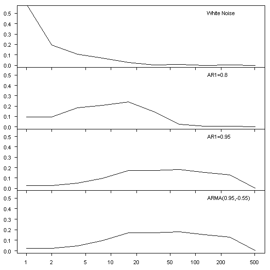
First, here are some illustrations of the variance at different scales (2^J) from wavelet decomposition of some simple processes. I like wavelet decompositions by scales rather than Fourier transforms, since variance by scale for red noise processes seems intuitively more meaningful to me than the frequency transforms and the summarization of information is more manageable. besides I’ve gotten used to it. The top panel shows white noise, with the majority of variance in the highest frequency. The second and third panels show AR1 examples – second with AR1=0.8 and third with AR1 =0.95, you see the increased loading around 10 years in the AR1=0.8 and between 16 and 256 years for AR1=0.95. For ARMA (0.95,-0.55), the variance distribution is very similar to the AR1=0.95 process. The ARMA (0.95,-0.55) combination is chosen intentionally as many processes often simulated as AR1 processes have a significant MA1 coefficient and with it a higher AR1 coefficient than in a simple AR1 model.

Figure 1. Illustration of variance in different scales under several processes.
The next figure shows the same decomposition for the average of PCs 1,2, 20 and 70 in the four panels from PC decomposition of a white noise network of 581 years long and 70 series. You can see that the series all have pretty similar variance allocations as the simple white noise example in the first figure.

Figure 2. Average Wavelet Variance Decomposition by Scale for PCs 1,2, 20 and 70 from white noise simulations (network 581 years x 70 series). Variances normalized to add up to 1.
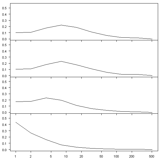
The next figure shows the same results for simulations based on red noise with AR1=0.6. Here you see loading at frequencies around 8-16 years in the early PCs, but white noise in the PC70. There are no actual "signals" in the data.

Figure 3. Average Wavelet Variance Decomposition by Scale for PCs 1,2, 20 and 70 from red noise (AR1=0.6) simulations (network 581 years x 70 series). Variances normalized to add up to 1.
The next figure shows the same results for simulations based on red noise with AR1 increased to 0.8. The variance loading is shifted a little towards lower frequencies with loading at frequencies around 16-32 years in the early PCs, but again white noise in the PC70.

Figure 4. Average Wavelet Variance Decomposition by Scale for PCs 1,2, 20 and 70 from red noise (AR1=0.8) simulations (network 581 years x 70 series). Variances normalized to add up to 1.
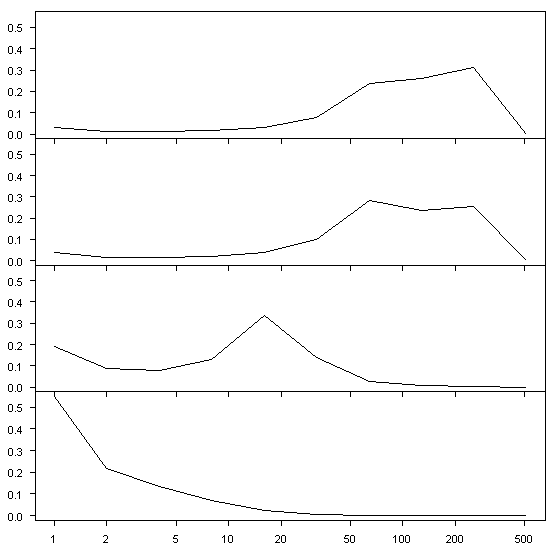
The next figure shows the same results for simulations based on red noise with AR1 increased to 0.95. The variance loading is shifted further towards lower frequencies with very significant loading at a "centennial" frequency of 128-256 years. The PC20 is loaded towards middle frequency, while the PC70 is loaded more towards high frequency.

Figure 5. Average Wavelet Variance Decomposition by Scale for PCs 1,2, 20 and 70 from red noise (AR1=095) simulations (network 581 years x 70 series). Variances normalized to add up to 1.
Finally, Figure 6 shows the same results for ARMA(1,1) with AR1=0.95 and MA1=-0.55. Again this generates considerable centennial variance in the early PCs. ARMA(1,1) processes often model out at about AR1=0.6-0.65 when modeled as AR1 processes, so you can see how much difference there is in low-frequency effects simply by the simulation model.

Figure 6. Average Wavelet Variance Decomposition by Scale for PCs 1,2, 20 and 70 from red noise (AR1=0.95,MA1= -0.55) simulations (network 581 years x 70 series). Variances normalized to add up to 1.
What does it all mean? I’m not quite sure. You’d think that this sort of stuff would be fully aired in the relevant literature before it is used in empirical studies, but such does not seem to be the case. While the MBH method is particularly bad, I get the impression that even conventional PC calculations are prone to identify low-frequency variability that does not exist in the data.


15 Comments
Wow… sounds like some updates to statistical methodology might be in order. Quite frankly, this type of thing makes me take any statistical presenation with a grain of salt.
If some methods “find” signals from noise, how can we trust any analysis that represents a signal mined from data using those methods?
Steve (and re# 1),
if you do want to make your own reconstruction, there is a relatively “hot topic” in neural computation, statistical signal processing and related fields called independent component analysis (and blind source separation in general). It just might be an appropriate technique for dealing with the type of data you’re interested in.
I’ve always regarded PCA as a step to decrease intercorrelation of variables by finding a set of axes that are most orthogonal. The current favored term for this seems to be data whitening. Perhaps one way of looking at it is to think of the PCA as as rotating the axes and data until the axes align with the data in a way that the major variance along each axis is perpendicular to all of the other axes. I think ICA provides a better method for doing this and often starts with PCA as a first step. Once a set of orthogonal axes is found, singularities in regression matrices become less likely.
I’ve never thought of using a PCA to find correlation. Is it possible that the above exercise simply shows that using a PCA for this purpose is mostly meaningless?
Some more thoughts:
I wish I could use a picture. I’d like to refer to an example that I saw when I first learned about PCAs. Perhaps I can illustrate it verbally. Imagine a scatter plot between two variables, V1 and V2, and that the resulting plot is an oval with the major axis of the oval lying on say the 45 degree line. PC1 would also lie on the 45 degree line while PC2 would be perpendicular to PC1 and aligned with the minor axis of the oval (135 degree line). The new origin would be centered in the middle of the oval cloud. With the exception that V1 and V2 might be completely independent, the resulting PCs would contain information from both variables. How then would any PC’s correspondence to either variable be meaningful?
The approach I would use would be to assume the different variables are independent signals (a possible fallacy) that have mixed to form the resultant measurement (tree ring thickness in the Mann case) which is modelled in a mixing matrix. I would pretend that each variable (temperature, CO2 level, amount of water, whatever) was a signal and each tree was a signal sensor. Unfortunately, while separating contributing sources, neither ICA nor PCA can identify which source is which. I would then have to use some other means to correctly assign the signal sources. Is this what has been done by Mann, et al. or did they try to correlate PC’s directly to the variables? Frankly, after reading the paper, I’m not actually sure.
In the above, if the sources are not independent, there is a strong possibility that any PCA or ICA is invalid.
Two things largely unrelated to this topic, but of some interest and there is no other place to post them:
(1) On the general public information front, the History Channel in the U.S. just ran a TV show on the Little Ice Age, fully acknowledging the MWP, and repeatedly stating that rather marked global (not just regional) temperature changes occur because of natural activity, not AGW. It even suggested the possibility of a future cooling period in the not so distant future.
(2) The show interviewed scientists relying heavily on oceanic sediment cores (rather than ice cores), measuring the ratio of warm organisms to cold organisms in the sediment, with the ratio providing accurate temperature trends. It said they demonstrated a 4-7 degree warmer MWP. I hadn’t seen those sediment cores heavily represented as proxies in Mann, et al. I’m wondering why. There’s probably a good reason. Perhaps too much granularity because of a lack of year-to-year tracking. But I thought it was interesting from an amateur point of view on the subject.
The graphs of the autogressive processes seem intuitive. While I don’t understand wavelets, I am interpreting the graphs akin to a regression fit (partial R-squareds) on sin functions of increasing period (decreasing frequency). For white noise there shouldn’t be much fit for long periods but lot for a period of 2. At the other end, for an AR(1) of 1.00, there should be lots of long runs relative the standard deviation of the process. Indeed the expected run is infinite — that’s one long cycle. For a finite length series one should expect to see a lot a the sin type curvature centering around a period of N/2. (At least I think it should be N/2.)
The long runs are going to have a lot more squared variation than the noise type behavior within the run, and thus the first principal component should be expected to pick up the period of those runs as opposed to the shorter period sawtooth behavior within the long runs. The greater the AR(1) coefficient the more likely the first PC is to be dominated by the long periods. Given a set of K series, there will be one with considerably longer apparent period than the average for the particular AR coefficient. This presumably is the reason for the greater period in the PC1 of the 70 series versus the distribution of variance in the typical series.
There is an analogy in regression of PCs on PCs. Take two sets of NxK series of white noise, X’s and Y’s. Run regressions of the individual series on individual series and you get the expected rejection rates on the coefficients for the X’s. Same holds for the PC1 of the Y’s on PC1 of the Y’s. But when you throw in serial correlation, say AR(1) = 0.8, the individual series will reject at roughly a 35% rate instead of the 5% rate of the classical model. That is an example of the standard “spurious regression” result. But the PC1 of the Y’s on the PC1 of the X’s will reject at 50%. Further, the PC(K), the last PC, on PC(K) will reject at a 15%, much closer to the classical mode. (These results are for a 400×40 set of Y’s and X’s. The effect will increase/decrease with the increase/decrease of the number of columns.) This exacerbation of the spurious regression effect could be interpreted as saying the PC1 removes the big changes, which are the long runs and hence long periods, and the sequential PC’s continue to “filter” out the remaining longest runs until the last PC is left with something that is most like white noise. Of course the “filtering” should not be taken literally since all the principal components can do is pick axes of the transformation in the data space.
These characteristics are what make principal components (and factor analysis) useful, but it is really not a technique that should be used to make regressors and regressands or any thing else to be used in subsequent squared distance minimization or maximization routine.
there’s an interesting article about wavelets in the current issue of the IEEE Signal Processing Society magazine. in particular, the concept of a dual-tree decomposition is discussed. i haven’t gotten into it yet (there are several other articles i’m even more interested in), but it doesn’t seem anything more involved than stripping off half-bands from each of the coefficient stages, i.e. perform hi/lo filtering at each stage on both the hi and lo coefficient sets. just another multi-rate filter bank i think.
to my surprise, btw, the article also referred to them as “bandpass” filters, which seems odd to me. i commented in another thread about this not being the case, but apparently i was mistaken (at least, mistaken that they are viewed in such a manner). i suppose the end-stage coefficients are indeed from a selected band, but individually they behave as lowpass and highpass pairs.
IMO, the primary reason for using any sort of wavelet analysis is that there are less people in the world that have even heard of it. the time-frequency characteristic is nifty, but not that much more nifty than a spectrogram. also, you’d still have the problem of weighting depending upon how you stitched the various proxies together.
mark
PS: i watched part of the LIA show, too. interesting things happened in an era that apparently didn’t exist according to bristlecone pine trees. 🙂
My sense also was that the PC1 is finding something like a sine-wave with a period related to a simple fraction of N. It sort of makes sense when you think about it, but it’s still entirely artificial.
It would be interesting to see the spectral composition of an AR 0.3 process, as some annual series leap straight from an AR 0.3 to an ARMA (0.9, -0.5).
I must admit however (as a non-economist)that I find ARMA a bit unsettling; one gets apparently highly significant coefficients yet the total residuals dont seem to reduce much. Looking at the big differences shown youve shown in your plots, makes me feel even worse!
Is there a simple metric that indicates how much more likely ‘model A’ (eg an ARMA) is to be true than say ‘model B’ ( an AR1)?
log likelihood and Akaiche Information Criterion are used. It’s dissatisfying to use criteria like this. I’m not sure of the “correct” way to handle these things. What does seem likely to me is that you can’t just ignore the error structure. The Hockey Team blithely assumes that everything is gaussian and independently distributely, when it isn’t. It seems to me that these ARMA(1,1) structures are common in climate time series. There’s a big difference in the properties of a model in which the series are AR1=0.3 and ARMA (0.95, -0.7) even if the distinction has to be done on log likelihood. Or at least, if you’re estimating confidence intervals, you can’t assume that everything is i.i.d. when the residuals have such a strong ARMA structure.
Re: 5 — you’re on the right track!
Haven’t seen the show, but selective sea sediment core choices could easily been made. Dr. Mann has already showed a preference for Dr. Keigwin’s Pickart’99 Newfoundland core (which statistically cools the MWP, and warms the LIA in multi-proxy), to Keigwin’s Sargasso Sea cores which show a pronounced MWP and to a lesser extent LIA. This was discussed in http://www.climateaudit.org/?p=145 — as was pointed out there, Monnin included Keigwin’s Sargassos ’96, and of course showed a MWP and LIA more in line which pre-HS thinking.
Sorry – this was mistakenly posted on another thread… should have been here.
Regarding next broadcast of LIA on the History Channel, is at 17:00 on 26-NOV (Saturday).
http://www.historychannel.com/global/listings/series_showcase.jsp?EGrpType=Series&Id=16021920&NetwCode=THC
NOTE: As part of the advertising teaser, the claim is it (the LIA) “decimated the Spanish Armada!” Oh well, looks like hyping the local WEATHER event impact of a changing global CLIMATE can happen on both ends of the temp scale.
Will we soon see a thread on how the show actually supports MBH’98 and ”
98 on RC.org?
According to the promo for the History Channel show, the LIA froze the Vikings in Greenland.
I made this point to William Connolley. He told me that
“….it wasn’t all green! just like now, it was mostly covered in ice!”
It seems that the Hockey Team believes that the Vikings colonized a glacier.
For the Vikings to colonize a glacier which was located several days’ sail from their nearest permanent settlement would be somewhat analogous to 21st century man establishing a colony on the moon. You would need to bring in most building materials and at least some of the food to keep the colony going. The logistics would have been daunting (without the MWP).
Correction to 11 — Moberg’05 (not Monnin) referenced Keigwin’96, and found more pronounced MWP and LIA.
Looking for some SVD/PCA applications I found this page. Theer are several papers dealing with distinguishing signals in red noise incl. on of mine 9with references to the other:
Title: Enhanced Monte Carlo Singular System Analysis and detection of period 7.8 years oscillatory modes in the monthly NAO index and temperature records
Author(s): Palus M, Novotna D
Source: NONLINEAR PROCESSES IN GEOPHYSICS 11 (5-6): 721-729 2004