Climate Audit

Wilson et al 2007 (previously discussed here) considers a Kyrgyzstan series that has numerous issues – the usual provenance problems unfortunately occur once again. But over and above that, it uses multiple inverse regression, a procedure used all too casually by dendros. In this case, the procedure flips over one of the ring width series and results in the reconstruction having a substantially higher 20th century trend than any of the constituent series. The form of multiple inverse regression is a little different than Mannian inverse regression and arguably even worse. Also when I replicated the recon using ITRDB chronologies, I got quite different (higher) results in the 18th century and no 20th century trend.

Here is the methodological description in Wilson et al 2007. (In fairness to the authors, they’ve at least given readers a fighting chance by giving ITRDB identification numbers. I’ve been trying for nearly 3 years now to get Hegerl, Crowley et al to identify the series that they used in the Urals and Mongolia without any success.) Wilson et al:

A search through the ITRDB, found surprisingly few temperature sensitive TR data sets that came up to at least 1995. Kyrgyzstan was one region where such chronologies were found (sampled and measured by the Swiss Federal Institute for Forest, Snow and Landscape Research). In this region, both RW and MXD data were obtained from two spruce (Picea shrenkiana) sites Sarejmek (ITRDB code: RUSS152, 41.36N 75.09E) and Tschongkys (RUSS164 42.11N 78.11E). Chronologies were computed using standard techniques. The period covered by at least 10 series in each chronology is 1689–1995. To account for the varying coherence between each chronology, the chronologies were not averaged to derive site mean series, but rather the RW and MXD chronologies were utilized separately as potential predictor series in a stepwise multiple regression against gridded temperatures. The final optimal model was calibrated against June–July mean temperatures, with the final series being a linearly weighted combination of the Sarejmek MXD and RW data as well as the RW data from Tschongkys. The final Kirgistan reconstruction explains 36% (r = 0.61. Table 1) of the gridded temperature variance.

I downloaded the russ152w, russ152x, russ164w and russ164x chronologies from ITRDB. [UPDATE: When I originally downloaded the chronologies in 2004, there was an error in the russ152w chronology which purported to show values well into the 21st century. In my original collation, I picked out the STD version from the Schweingruber data set (which has three versions), but when I re-visited this matter a few days ago, I inadvertently picked out the first version, which, as pointed out by Craig Loehle and Rob Wilson below, was not the STD version. I’ve re-done the collation, this time picking out the STD version of the russ152w chronology and done calculations with this. Rob Wilson kindly sent me his versions which enabled a prompt reconciliation – his measurement data set did not use 4 cores in the russ152w.rwl but the match is now close. Subsequent paragraphs have been re-stated to reflect this reconciliation on the basis. ]

I did a usual reverse engineering regression in which I regressed the Wilson KYR reconstruction against the constituent chronologies, using both the 4-series and 3-series combinations. Given that the final series is supposedly a “linearly weighted combination” of the russ152w, russ152x and russ164w series, the R^2 from this regression should be 1 or very close to it. The adjusted r^2 is 0.92 (improved from 0.78 previously reported). Note the negative coefficient on the russ164w series: this series has been flipped over in the reconstruction.

(Intercept) 0.04224 0.01783 2.369 0.0186 *
russ152w 0.61866 0.02265 27.310 <2e-16 ***
russ152x 0.66404 0.02672 24.854 <2e-16 ***
russ164w -0.54274 0.02154 -25.202 <2e-16 ***
russ164x -0.03597 0.02724 -1.321 0.1879
—
Signif. codes: 0 ‘***’ 0.001 ‘**’ 0.01 ‘*’ 0.05 ‘.’ 0.1 ‘ ‘ 1

Residual standard error: 0.2789 on 241 degrees of freedom
(135 observations deleted due to missingness)
Multiple R-squared: 0.9254, Adjusted R-squared: 0.9242
F-statistic: 747.5 on 4 and 241 DF, p-value: < 2.2e-16

Using the ITRDB versions available to me, I attempted to replicate Wilson’s stepwise methodology as follows. First I did a multiple inverse regression of CRU gridcell temperature (42N, 77E) against all 4 chronologies:

fm=lm(cru~.,data=Z[,1:5])
summary(fm)

This yielded an adjusted r2 of 0.27 using the russ152w STD chronology(versus 0.36 with the russ152w RAW) with three “significant” coefficients, including a flipped russ164w.

Coefficients:
Estimate Std. Error t value Pr(>|t|)
(Intercept) -0.48103 0.08636 -5.570 1.85e-07 ***
russ152w 0.33073 0.11410 2.899 0.004533 **
russ152x 0.44390 0.13098 3.389 0.000977 ***
russ164w -0.38271 0.11170 -3.426 0.000864 ***
russ164x 0.03474 0.12550 0.277 0.782466
—
Signif. codes: 0 ‘***’ 0.001 ‘**’ 0.01 ‘*’ 0.05 ‘.’ 0.1 ‘ ‘ 1

Residual standard error: 0.9197 on 109 degrees of freedom
(267 observations deleted due to missingness)
Multiple R-squared: 0.298, Adjusted R-squared: 0.2722
F-statistic: 11.57 on 4 and 109 DF, p-value: 7.3e-08

I then used the stepwise regression function in R (step):

fm0=step(fm)

This yielded a model selecting the three series noted up by Wlson, again with a flipped orientation for the russ164w series.

(Intercept) russ152w russ152x russ164w
-0.4800288 0.3244294 0.4696676 -0.3770913

Using the archived series, I ended up with a “reconstruction” that has a correlation of 0.54 (0.62 with russ152w RAW) to the gridded series, somewhat lower than the reported correlation of 0.61 (although I got 0.62 for the Wilson version against present CRU3). The emulation has a fairly similar appearance to the Wilson version, both being shown below, but there are also some notable differences.

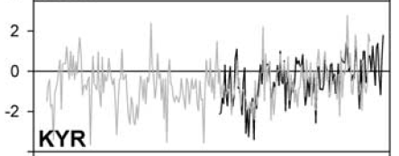
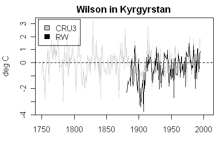
Top – Excerpt from Wilson et al 2007 Figure 3; bottom – emulated from ITRDB data.

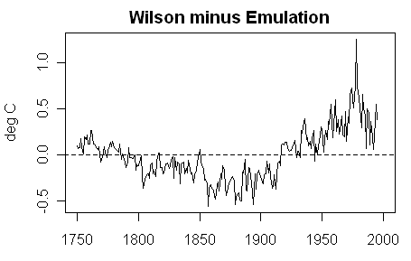
The next graphic shows a plot of the residuals between the re-stated Wilson emulation and the archived Wilson version, which remain very noticeable even after the reconciliation accomplished so far.

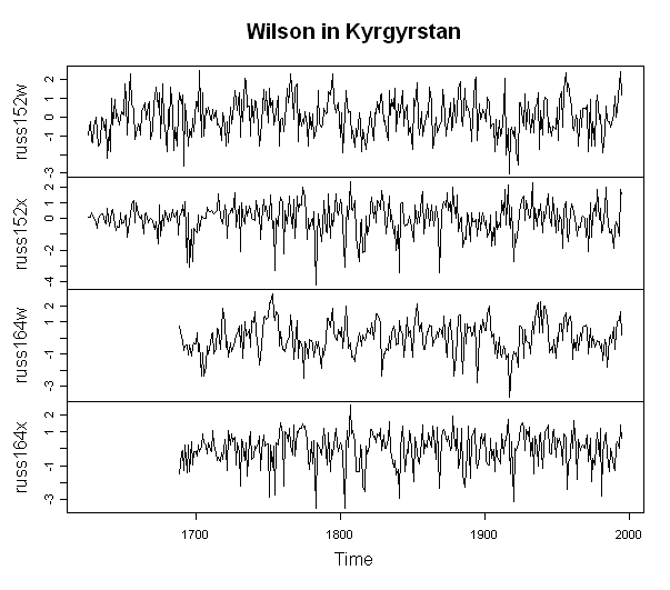
Here is a re-stated plot of the 4 candidate constituent series, plotted from data downloaded from ITRDB with the russ152w STD now shown.

I calculated the 1920-2000 trends for scaled versions of each of the 4 constituent series (scaling in order to make comparison to CRU easier). Three of the 4 series had negative trends in the 1920-2004 period; only russ152w had a positive trend in this period ( 0.006366476 SD Units/year). My emulation of the Wilson method yielded a reconstruction with virtually no trend ( 0.002264408 SD Units/year), but the Wilson reconstruction had an observable positive trend in the 1920-2004 period (0.008109656 SD units/year), which was greater than the trend of any of the constituent series.

Finally, as an exercise, I calculated ARMA(1,1) coefficients for the constituent series. For the russ152w STD series, the ARMA(1,1) coefficients were much reduced from the russ152w RAW version (which was close to a random walk), but the coefficients were both highly significant. For many series, I’ve found that an ARMA(1,1) model is highly significant relative to an AR1 model and always results in a much higher AR1 coefficient combined with a negative MA1 coefficient. This is characteristic of a wide variety of climate series.

# ar1 ma1 intercept
# 0.6708 -0.4867 0.0019
#s.e. 0.1298 0.1505 0.0784

UPDATE:

Rob Wilson sent me the chronologies that he used for Kyrgyzstan and differences arise almost entirely from differences between Rob’s re-calculated chronologies and the ITRDB chronologies, which end up imparting very substantial differences to the overall result.

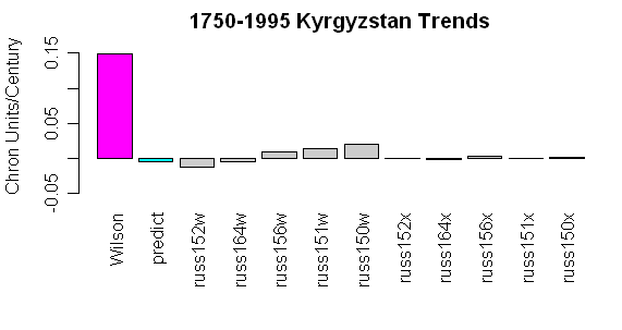
First here is a graphic comparing the 1750-1995 trends for Wilson’s Kyrgyzstan composite and 10 Schweingruber Kyrgyzstan chronologies, of which Wilson used 4 (3 after stepwise).

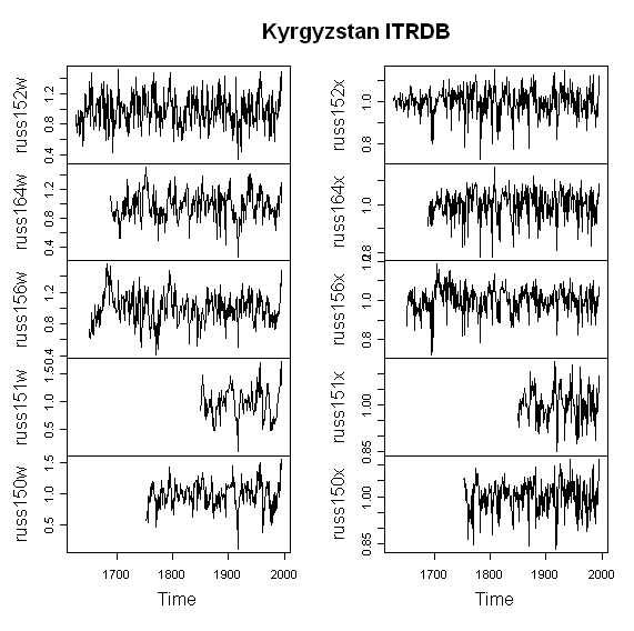
Plots of all 10 Kyrgyzstan STD chronologies as archived at ITRDB are shown below, and the lack of trend is obvious.

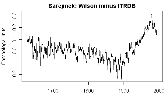
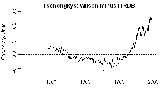
Rob sent me the chronologies as he calculated them for the sites that he used. Below are plots comparing Rob’s chronologies to ITRDB chronologies – in both cases, Rob’s chronologies have a greater 20th century increase than the ones at ITRDB.

Rob said that he had “no idea what detrending methods were used to derive the ITRDB version – hence I would never use it”. Fair enough. But this is the same problem that I’ve complained about over and over again in this trade. Appendix A6 says only:

Chronologies were computed using standard techniques.

As Rob observes below, Appendix 3A discussing Scandinavia states:

These chronologies were detrended using so-called standard techniques (either negative exponential or regression functions of negative or zero slope).

and in an email, Rob stated to me that this applied to Kyrgyz as well. I’m sure that ITRDB would also say that they used so-called “standard techniques”, but their definition obviously differs somewhere from Rob’s. They have relatively recent (June 2005 report) on the chronology here . If Rob is unable to determine from June 2005 meta-data how the chronology was done, thereby making it unusable, then ITRDB need to do a better job; this is a facility for dendros and shouldn’t they take some responsibility for the defective metadata?