The bias arising from ex post selection of sites for regional tree ring chronologies has been a long standing issue at Climate Audit, especially in connection with Briffa’s chronologies for Yamal and Polar Urals (see tag.) I discussed it most recently in connection with the Central Northwest Territories (CNWT) regional chronology of D’Arrigo et al 2006, in which I showed a remarkable example of ex post selection.
In today’s post, I’ll show a third vivid example of the impact of ex post site selection on the divergence problem in Gulf of Alaska regional chronologies. I did not pick this chronology as a particularly lurid example after examining multiple sites. This chronology is the first column in the Wilson et al 2016 N-TREND spreadsheet and was the first site in that collection that I examined closely. It is also a site for which most (but not all) of the relevant data has been archived and which can therefore be examined. Unfortunately, data for many of the Wilson et al 2016 sites has not been been archived and, if past experience is any guide, it might take another decade to become available (by which time we will have all “moved on”).
The 2006 and 2014 Chronologies
In this case, the Gulf of Alaska chronology of D’Arrigo et al 2006 was the first long chronology using mountain hemlocks (TSME) from the Gulf of Alaska coast. It had a pronounced divergence problem (top panel) and was never reported in a technical publication. In 2007, Wilson et al published a second long chronology, which purported to somewhat mitigate the divergence problem. (See Postscript). In 2014, Wiles et al published a third long Gulf of Alaska TSME long chronology (later used in Wilson et al 2016), which was virtually identical to the 2006 version through its early history up to the 18th century or so, but which goes up in the 20th century, seemingly avoiding the divergence problem of the earlier series:
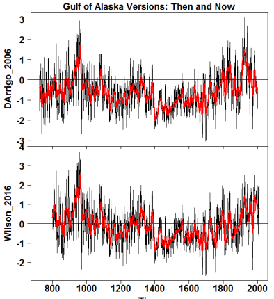
Figure 1. Gulf of Alaska TSME regional chronologies: top – D’Arrigo et al 2006; bottom – Wiles et al 2014, as used in Wilson et al 2016.
Effect of Site Selection
Both Gulf of Alaska chronologies (D’Arrigo et al 2006 and Wiles et al 2006) used the same two subfossil data sets: both on the coast of Prince William Sound to the left of the location map shown below as Figure 2 (shown in large red-pink icons). The identity of subfossil data explains the remarkable similarity of the two versions of the chronology up to about the 18th century: they are similar because they used the same data in this period.
However, the modern portion of the chronologies differs: the D’Arrigo et al 2006 version has a divergence problem, whereas the Wiles et al 2014 does not. Both D’Arrigo et al 2006 and Wiles et al 2014 used RCS variations, but Wiles et al only used three (yellow) of ten D06 sites; Wiles et al discarded seven sites used in D’Arrigo et al 2006 (red below) and added five sites not used in D’Arrigo et al (green). The D06 sites were first listed in the D’Arrigo et al 2006 Supplementary Information in 2012, over seven years after the article was cited by IPCC.
Remarkably, nearly all of the modern sites discarded by Wiles et al (red pins) are located close to and even almost contiguous with the two subfossil sites (both near the coast of Prince William Sound), while the five sites added by Wiles et al are all located about 800 km away near Juneau.
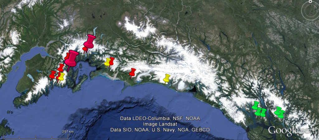
Figure 2 Location map comparing sites in D’Arrigo et al 2006 and Wiles et al 2014. Large red-pink – two subfossil sites used in both studies; red- seven modern sites only used in D’Arrigo et al 2006; yellow- three modern sites used in both studies; green – five modern sites only used in Wiles et al 2014.
The only information in D’Arrigo et al 2006 on the provenance of their Gulf of Alaska data was that they used 820 cores and that its reference was “Wiles et al., Tree-ring evidence for a medieval warm period along the southern coast of Alaska, manuscript in preparation, 2005.” Unfortunately, this article never appeared and, to my knowledge, there was never any technical publication of the D’Arrigo et al 2006 Gulf of Alaska series. In 2012, an amendment to the D’Arrigo et al 2006 Supplementary Information finally listed the sites used in the D06 Gulf of Alaska regional chronology (used in the above location map.)
Wiles et al did not reconcile their sites against the sites previously used in D’Arrigo et al and, based on the location map, it is very difficult to contemplate a plausible ex ante rationale. Indeed, it is hard to think of any rationale for the 800 km migration other than an intent by Wiles et al to “partially circumvent” the divergence problem by only using modern sites that went up, a program described in D’Arrigo et al 2009, (quoted in the previous post) as follows:
The divergence problem can be partially circumvented by utilizing tree-ring data for dendroclimatic reconstructions from sites where divergence is either absent or minimal. (Wilson et al., 2007; Buntgen et al., in press; Youngblut and Luckman, in press).
And, indeed, the divergence problem was definitely on the minds of Wiles et al. In their abstract, they stated that the modern sites in their network showed no “evidence of the so-called divergence effect”. They attributed this to the “moderate elevation” of the sites in their selection of sites:
The moderate elevation at the tree-ring sites has allowed these trees to retain their temperature signal without evidence of the so-called divergence effect, or underestimation of tree-ring inferred temperature trends, which is observed at many northern latitude forest locations.
Later, in the running text, they explained that they “target[ed]” sites where the “trees appear to still be responding positively to temperature” to avoid “bias[ing]” their results:
Here, we use tree-ring records from living hemlock at mid-elevation GOA sites where such trees appear to still be responding positively to temperature as in the past. Targeting such sites, we minimize divergence in the recent period that might bias our results and thus provide a more accurate assessment of contemporary warming relative to previous centuries.
It was either cheeky or ignorant on their part to characterize such blatant cherrypicking as a technique to avoid “bias[ing] their results”. That such strategies are accepted without qualm both by referees and other specialists in the field speaks volumes.
A Replication Puzzle
Even spotting Wiles et al their modern sites, I do not believe that it is possible to replicate their non-declining chronology based on available data.
Wiles et al used 8 modern sites and two subfossil sites (listed in their Table 1). Measurement data for the two subfossil sites and six of eight modern sites appears to be fully archived at NOAA, but one data set (Wright Mountain) is completely unarchived and an unarchived (and expanded) second version of Eyak Mountain appears to have been used in Wiles et al 2014. Ironically, Wiles et al 2014 Table 1 specifically (but incorrectly) stated that the Wright Mountain data had been archived at ITRDB.
Nonetheless, the archived data for the two subfossil sites and 6.5 (of 8) modern sites permits calculation of an RCS chronology that would one would expect to be quite similar to the chronology reported in Wiles et al 2014. Using the available data, I therefore calculated an RCS chronology (see bottom panel) using a one-size-fits-all standardization curve, an RCS variant said to have been used, according to the running text of Wiles et al 2014. The correspondence between the Wiles chronology and my emulation is very close up to the 18th century, but I was unable to replicate the closing uptick of the Wiles et al 2014 reconstruction, obtaining instead the closing decline, also seen in the D’Arrigo et al 2006 version.
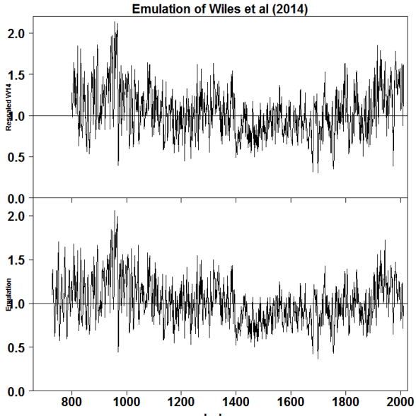
Figure 3. Top – Wiles et al 2014 reconstruction re-scaled to match chronology scale; bottom – emulated RCS chronology using available ITRDB data for sites listed in Wiles et al Table 1.
In the next figure, I’ ve tried to highlight the 20th century difference between the two versions by zooming in. At high frequency, the Wiles et al version and the emulation are very similar, but the emulation (red) shows the characteristic decline (divergence problem), while the Wiles version goes up slightly in the 20th century, with most of the increase due to higher post-1975 values in the Wiles reconstruction.

Figure 4. Detail of chronologies shown in Figure 3.
It is possible that inclusion of the unarchived data from Wright Mountain and Eyak Mountain will reconcile the differences; if so, there is considerable irony in the proposed mitigation of the divergence problem depending on only two sites, neither of which have been archived. It is possible that the difference arises in different implementations of poorly described RCS protocols – maybe the chronologies were estimated site by site and averaged, rather than one size fits all. There is one final possibility that I would never have postulated prior to my recent reconciliation of the D’Arrigo et al Central Northwest Territories regional chronology: in that case, D’Arrigo selectively included cores from a site that went up, while selectively excluding cores from a site that went down. Without a complete measurement archive, there is little point reflecting further on such matters.
Conclusion
My underlying issue with “regional chronologies” is that the 20th century shape of the chronologies can be dramatically impacted by ex post selection of modern data. I originally raised the question of ex post data collection in the earliest days of Climate Audit in connection with the NH reconstruction of Jacoby and D’Arrigo 1989. I wrote many posts on this issue in connection with Briffa’s Yamal and Polar Urals chronologies, where site selection clearly impacted the shape of the chronology (see e.g. here here here here here.) This was a large controversy leading into Climategate.
In a recent post, I showed that D’Arrigo consciously attempted to “circumvent” the divergence problem by ex post selection of sites that went up, with a surprisingly blunt implementation of this questionable strategy in the CNWT regional chronology of D’Arrigo et al 2006. In today’s post, I showed that the Gulf of Alaska regional chronology is one more example, where the shape of the regional chronology has been impacted by ex post site selection, in this case, with the selective use of sites over 800 km distant from the target subfossil sites.
Some time ago, Gavin Schmidt observed of a chronology of which he disapproved (his objections not actually being valid, but that’s another story):
if any actual scientist had produced such a poorly explained, unvalidated, uncalibrated, reconstruction with no error bars or bootstrapping or demonstrations of common signals etc., McIntyre would have been (rightly) scornful.
Even though that the most recent Gulf of Alaska chronology amply meets Schmidt’s criteria of being “poorly explained, unvalidated, uncalibrated, reconstruction with no error bars or bootstrapping or demonstrations of common signals”, I will content myself with mild (Canadian) disapproval, but would not strongly argue with Schmidt if he wrote a review that was more severely “scornful”.
Postscript – Wilson et al 2007
In 2007, Wilson et al published a third regional chronology using Gulf of Alaska TSME sites. While this chronology was not used in the Wilson et al 2016 composite, the Supplementary Information of D’Arrigo et al 2006 stated that the cores used in D’Arrigo et al 2006 were identical to the cores used in Wilson et al 2007. I have concluded that his information is false, but it took me quite a bit of time to be confident of this conclusion and I wish to document my reasoning while it is fresh in my mind.
Wilson et al 2007 had been discussed at Climate Audit soon after publication (also here on varimax rotation). Needless to say, the measurement data required for analysis was not available at the time of publication. The comments thread contained a lively exchange between Willis Eschenbach and Rob Wilson about archiving: Eschenbach sharply criticized Wilson and coauthors for failing to archive data concurrent with publication; Wilson attempted to deflect the criticism as overwrought on the grounds that archiving delay, while regrettable, would be slight. As it turned out, the majority of the missing data wasn’t archived for another five years (2012) and a little is still unarchived, a delay which, in my opinion, more than vindicates Eschenbach’s side of the dispute.
In fall 2009, Kaufman et al (2009) published a multi-proxy Arctic reconstruction, one item in which was a Gulf of Alaska temperature reconstruction attributed to D’Arrigo et al 2006 (which had produced an RCS chronology but not a temperature reconstruction.) In December 2009, the Supplementary Information to D’Arrigo et al 2006 was amended, including the archiving of the Gulf of Alaska temperature reconstruction used in the recently published Kaufman et al. (All other D06 chronologies remained unarchived until 2012!!)
The 2009 SI amendment stated that the D06 Gulf of Alaska chronology had used the same 820 cores as the Wilson et al 2007 reconstruction:
Wilson et al. 2007 produced a Gulf of Alaska reconstruction based on an STD chronology derived from the same 820 ringwidth series….
820 individual series that were published in the two articles listed above. The Standard Chronology (ak096.crn) was used for the reconstruction by Wilson et al. 2007. The RCS chronology (ak096c.crn) was used in the D’Arrigo et al. 2006 reconstruction.
At this time, two chronologies (ak096.crn and ak096c.crn) and one measurement dataset (ak096.rwl) were contributed to the ITRDB data bank.
However, Wilson et al 2007 (of which Wiles was a coauthor) described an entirely different network that that illustrated in my Figure 2 (based on my reconciliation of the core numbers of ak096.rwl. Wilson et al listed an opening network of 31 sites in their Table 1. Wilson et al appear to have calculated RCS chronologies on a site-by-site basis for all 31 sites, which were then screened for correlation to instrumental data, resulting in nine sites being discarded. The 31 Wilson et al 2007 sites were shown in a location map in the original article, reproduced and annotated below, showing a stretch of the Alaska coastline almost 1000 km long, reaching from the Juneau area on the right to Kodiak Island on the left:

Figure 5. Location map from Wilson et al 2007, showing the 31 sites (22 used sites in solid colors), overprinting the D06 sites (magenta +).
In 2012, more major changes were made to the SI to D’Arrigo et al 2006. Seven years after my request to IPCC, the 19 regional STD and RCS chronologies were finally archived. While the STD and RCS chronologies archived in 2012 for Gulf of Alaska matched the two ak096 chronologies archived in 2009, the chronologies for most of the sites appeared in 2012 for the first time. New 2012 commentary on the Gulf of Alaska chronologies stated that the D06 chronology had been developed from 10 modern sites:
Coastal Alaska
10 Living chronologies:

Data with ITRDB code:
Ellsworth Glacier, Alaska (EL)	ITRDB AK015
Rock Glacier (RG)		ITRDB AK024
Water Supply (WS)		ITRDB AK029
Wolverine Glacier (WV)		ITRDB AK030
Tebenkof Glacier (TB)		ITRDB AK025
Miners Well (MW)		ITRDB AK021
Nichawak Mountain (NK)		ITRDB AK022
Cordova Eyak Mountain (CV)	ITRDB AK020
Massive Rock near Cordova (MR)	ITRDB AK090
Rock Tor (RT)			ITRDB AK091

Sub-fossil material: Data not archived and continually being updated.
Relevant contact is Greg Wiles (gwiles@xxx) – primary generator
of the data - and Rob Wilson (rjsw@xxx) who has original
2006 version used.
I’ve marked the location of these sites used in D’Arrigo et al 2006 with a magenta + sign. Nearly all of the 10 come from the Prince William Sound area (top towards the left), whereas the W2007 sites stretch for about 1000 km along the coast. The two subfossil sites (used in all long chronologies) both come from the Prince William Sound area (marked with solid magenta dots). Ironically, although the 2012 SI amendment said that the subfossil data was not archived, it had actually been archived in 2009 (as part of ak096.rwl).
Obviously , the 10 modern sites used in D’Arrigo et al (2006) do not match the 22 modern sites used in Wilson et al 2007. Only nine sites are common. Thirteen sites used in Wilson et al 2007 are not used in D’Arrigo et al 2006, while one site used in D’Arrigo et al (Tebenkof Glacier) was not used in Wilson et al 2007. It is obviously impossible for the 820 cores used in D’Arrigo et al 2006 to be identical to the cores used in Wilson et al 2007, unless the descriptions in Wilson et al 2007 are completely incorrect.
It is also instructive to review the multivariate methodology of Wilson et al 2007 as a potential contributor to their “circumventing” the divergence problem. After they had screened their original network from 31 to 22 sites – ex post screening of the type long criticized at Climate Audit, they carried out principal components analysis on the 22 site-by-site chronologies (each of which was calculated as a site STD chronology). They retained four principal components, which were then subjected to varimax rotation. They then calculated a temperature reconstruction by regressing instrumental temperature onto the four (rotated) principal components in a calibration period. The resulting temperature reconstruction (not shown in this post, but its shape is similar to the Wiles et al 2014 reconstruction shown above) did not have the 20th century decline that characterized the Arrigo et al (2006) reconstruction.
In a recent discussion at Bishop Hill, Rob Wilson likened the improvement in recent regional chronologies to the improvement from a Trabant to a 2016 BMW Series 1:
Of course there are older versions, but only a fool would use an old version with less data or that had calibration issues etc. Would you rather drive a Trabant or a 2016 BMW series 1. Duh!
Each of the multivariate operations in their PC methodology is linear and thus the temperature reconstruction is necessarily a linear function of the underlying 22 chronologies. However, the technique of Wilson et al (2007) does not constrain the coefficients to remain positive. Their method can result in negative coefficients i.e. flipping of series upside down (an issue that Jeff Id and I have discussed on many occasions in the context of Mannian methodology). Even if it is possible to extract information on regional temperature from the tree ring data, in my opinion, complicated multivariate methods like that of Wilson et al 2007 are a retrogression from simpler regional averages, rather than an improvement – let alone an improvement on the order of a Trabant to a BMW Series 1 – unless one were attempting to quantify “improvemens” in the technology of “data torture”.


129 Comments
The moderate elevation at the tree-ring sites has allowed these trees to retain their temperature signal without evidence of the so-called divergence effect, or underestimation of tree-ring inferred temperature trends, which is observed at many northern latitude forest locations.
Although logically delusional, perhaps we can take from this a tacit burial of the treeline treemometer kindergarten of thought. I.e., the divergence problem is big for latitudinal treeline rings, and probably the altitudinal ones too. Their solution: 1. find some trees that fit, 2. assess their elevation, 3. vacuously assert said non-treeline elevation produces better treemometers. (Gaspe…”moderate” elevation too??)
we minimize divergence in the recent period that might bias our results
Wow.
“…Targeting such sites, we minimize divergence in the recent period that might bias our results and thus provide a more accurate assessment of contemporary warming relative to previous centuries…”
Priceless. Divergence is a bias, but selection bias is not a bias?
“…It is possible that inclusion of the unarchived data from Wright Mountain and Eyak Mountain will reconcile the differences…”
Yeah, “possible.” You’re too kind. The shape of Wiles et al 2014 and your emulation match so very well. It would seem remarkable that the inclusion of unarchived data would retain almost the identical shape and yet shift the composite data to match your emulation. At face-value, it seems more like some undescribed processing or “poorly described RCS protocols” were performed.
But even if it were just a case of incorporating unarchived data, you’re right – how ironic. I guess it just goes to show how “robust” (I am so tired of reading that word describing garbage) or not the results really are.
Steve: prior to determining that D’Arrigo had cherrypicked individual trees in the CNWT regional composite, I would considered that cherrypicking was limited to the selection of sites, but not at a tree level. Right now, it’s hard for me to see how Wiles could have got his 2014 version without cherrypicking at a tree level.
” Right now, it’s hard for me to see how Wiles could have got his 2014 version without cherrypicking at a tree level.”
Wouldn’t that be the logical extension of the original ex post screening philosophy? If a whole site is “unsuitable” because of divergence, why wouldn’t an individual tree also be considered by the same criterion?
But how are the trees doing as thermometers, has anybody ever compared regional tree rings with regional temperatures?
Hans, usually they are calibrated using regional temperatures. So comparisons go pretty well after that is done 😉
Do you have an example? And some correlation statistics?
Hi Hans,
This is MXD and not ring width, but an amusing one, as the authors fret that these trees just can’t seem to replicate warmer temps…
PDF here http://www.ldeo.columbia.edu/~jsmerdon/papers/2015_grl_schneideretal.pdf
Link to supplemental info in a Word doc here that has some stats (Pearson r on page 3, for example)
http://onlinelibrary.wiley.com/doi/10.1002/2015GL063956/full
-Mike
For those interested – 2007 paper here:
Click to access Wilsonetal2007a.pdf
In the 2007 study, RCS was not used to detrend the data. It states quite clearly:
“To remove non-climatic biological age-related
trends (Fritts 1976), the individual raw ring-width series
were detrended using negative exponential functions
or regression lines of negative/zero slope (Cook
and Kairiukstis 1990). For 12 of the chronologies (DM,
WP, RG, EX, LL, MR, NK, TM, MW, AP, MT and
KI), the Cook and Peters (1997) power transform was
used to reduce end effect inflation of resultant indices
in some select series.”
The focus of the study was on multi-decadal variability so the processing of the data was quite different to the regional GOA RCS chronology used in DWJ06. The full GOA recon shown in Figure 9a does not express any longer term secular variability as that has been removed via detrending.
Yes – I did screen the data against the large regional temperature series. Agreed that this could lead an inflated r2 value – easy to test. However, one thing you have not stated is that the sub-fossil chronology extension IS a simple mean and that compares rather favorably with the PCregression living reconstruction – see Figure 7. I would see that as a form of validation.
Rob
Steve: Thanks for the comment. I changed a few words in the relevant sentence of the postscript to note that the 22 screened chronologies used STD methods. Thanks for observing this. This point about Wilson et al 2007 does not affect the cherrypicking argument, nor does it affect the observations of the multivariate method of Wilson et al 2007. I value the ability to both agree and disagree with Rob civilly.
Rob: started to digest the article you to which you were kind enough to provide a link.
One quick question: I noticed that you relied on a few data sets that were published by D’Arigo…any diem if she employed the type of post hoc selection of the members of those data sets that she has endorsed?
“Agreed that this could lead an inflated r2 value”
Is there some possibility that it would not lead to inflated agreement? – My answer is no so a test is not required.
What this screening is, is an ad-hoc form of regression utilizing binary (1 or 0)weighting. All of these regression methods do the same thing they just have different weightings.
What many of us are stating is that the practice is completely invalid, what I would like to have is an explanation of how we are wrong. We have all been looking for a rational explanation for years, and cannot get a serious answer.
I absolutely and totally agree not just with the overall point, but with this way of expressing the point.
yet Rob, in his article explicitly states that he does this.
How can it be that so many in this subdiscipline are so bereft of the most cursory and superficial understanding of the foundations off statistical analysis?
His own efforts entail “calibrating” his data to the instrumental record, and discarding those times series that dont correlate well with it, with no real rationale other than they somehow aren’t magic enough to convey some temperature signal…
Prof. Wilson:
How did you control for the wide range in local precipitation across the Gulf of Alaska? Your paper discusses temperature correlations with the PDO and NPI but I could find no discussion of precipitation other than a suggestion that several of the discarded sites were potentially in “drier” locations.
For those who are unfamiliar with the region, micro-climates abound. Annual precipitation among locations varies by several meters (yes, meters). As a result, using records from, say, Sitka or Juneau would not necessarily reflect the local precipitation (or temperature?) at tree-ring sites.
Specifically, your reference to drier locations notes that some discarded chronologies:
If one assumes, as implied by the quote, that “influence” from the North Pacific results in increased precipitation, how did you control for this factor when attempting to extract the similarly influenced temperature signal?
And thank you for providing the link to your paper and your willingness to engage in the discussion.
Kent
It would appear that SteveM’s examples of selecting proxies after the fact and explaining the problems that that incorrect procedure causes will continue to fall on deaf ears in the dendro community. Would not it be great to hear a member of that community delve into the basic statistical issues and biases that post selection creates? Too many who discuss these issues, and from all sides of the validity issue, seem at some point to get distracted with other details of dendro investigations and papers that deal with temperature reconstructions. Pure and simple is it that without a valid prior selection process for proxies the reconstructions are not valid – even if accepted within the community as such.
Even if one wants to ignore that basic selection problem and point to correlation coefficients between temperature and tree rings or tree rings reactions to temperature pulses such as from volcanic eruptions there remain statistical problems there.
Tree rings obviously react to temperature and unfortunately to a number of other variables that can be climate or non climate related. If, and this is a mighty big if, those other variables were occurring over time in a random fashion it would be expected that a sufficiently large sample would have those variables cancelling out. But by that reasoning all prior selected samples would have to be used from the range of temperature responses that would be expected. An after the fact selection would ruin the cancellation process.
It is sometimes shown that tree rings react to volcanic pulses and this should not be unexpected as a sudden large change in temperature would tend to dominant over the other variables. The problem here is that the amplitude of those responses are not necessarily in portion to the expected temperature change. This reaction leads to another issue of high and low frequency responses of tree rings to temperature. A low frequency response from tree rings is probably what is needed for validating the tree ring as a reasonable thermometer for climate science as it is the trend in temperature that is the important feature. The problem with that relationship between temperature and tree response is that with two time series with large auto correlations an artificial and false correlation can be found with reasonably high statistical probability depending on the amount of auto correlation. On the other hand qualifying a tree ring proxy by its high frequency response to temperature can lead to a reasonable correlation that can actual have a divergence in trend – which is back to case of the tree ring responding in direction to temperature but not in proportion to the change in temperature.
If SteveM were to present a quiz here on all these issues I would predict that no dendros would be takers and many of those who might call themselves skeptical of the validity of tree ring temperature reconstructions would fail or do poorly.
Thanks for reiterating this point.
If one cannot, before the act, articulate a process and a rationale for discarding data, then what is happening is a post hoc selection of data that agree with one’s hypothesis…nothing more nothing less.
Ok Kenneth
here is a question for you, david, craig, mc.
prior to test I establish my selection criteria ( environmental ect ) and
i include in this selection criteria RW correlation to local temperature, even the most crude type of correlation metric.
When it comes to reconstructing, however, I use density.
Steve Mc: I don’t have a clue what your question is here. Look, a proxy for temperature is supposed to have a correlation to temperature. Thermometers work because their physical properties correlate to temperature. The point is that – as I’ve discussed over and over – if you believe that white spruce chronologies at treeline (or whatever) are temperature proxies and you go and collect 31 of them, then you have to use all 31 in your study. You can’t de-select “divergent” chronologies ex post. Again, consider the situation of a portfolio. He can’t redo his portfolio afterwards. Surely this isn’t what you’re talking about.
Steve:
since you posted this and addressed it to me, among others, i will take a swing at responding to your post:
“here is a question for you, david, craig, mc.
prior to test I establish my selection criteria ( environmental ect ) and
i include in this selection criteria RW correlation to local temperature, even the most crude type of correlation metric.
When it comes to reconstructing, however, I use density.”
Is there a question in your comment?
I dont see one.
Im pretty certain that disregarding any data in your sample after you collected it because it didn’t correlate with local temperature is a post hoc selection of data, even if one uses density for the reconstruction… is this not true?
In the end, aren’t you going to use density because it…correlates with local temperature?
Are you implying that tree density is somehow correlated to something other than local temperature?
Why the “Tennessee Two Step”?
You may understand programming in R, but this key concept (post hoc selection) seems to escape you.
And, BTW, what would be your concept of “the most crude type of correlation metric”?
Isn’t this a situation with one dependent and one independent variable?
Is there a more simple scenario in which one would wish to compute a correlation coefficient between two variables?
The only rational reading of your selection criteria is that you establish that the only tree rings you will include are those that correlate to local temperature…
you are then going to use these data to show what?
that they are correlated to local temperature?
geez mosh.
I think the problem is that referring to ex-post suggests the problem arises because you are discarding having eye balled the results. This is of course a problem, but you will have potential problems with inference off a sample that is systematically biased by any selection criteria.
Take an analogy. We know the weight over time of members of a community and for a period we know the general level of deprivation faced by it and we want to estimate this in times gone by. Ex-ante we specify that we will only use those members of the community where there is 95% significant correlation between the deprivation and weight measure (or if we’re Steven Mosher we say height and deprivation). No ex-post funny business.
But the problem is that we want to get an estimate of the deprivation the community faced, not the deprivation these individuals faced. This subsample is very likely not representative within sample, let alone useful for drawing inferences out of sample.
An example is that individual weight vulnerability/sensitivity to deprivation at a given time is likely to a function of a wide range of other factors. Self-sacrifice by older community members would be an example. Assuming the same relationship applies when they are much younger would be quite wrong.
So it isn’t just ex-post selection, it is the risk of bias from any selection process that isn’t random within the population of interest.
“i include in this selection criteria RW correlation to local temperature,”
Substitute “the price of gold” for “local temperature.”
It seems to me that if your selection criteria is correlated to what you are looking for then you are going to find it, right?
Okay I think I see what Steven Mosher is doing. Correlate to ring WIDTH and then reconstruct against ring DENSITY, implying that ring width is independent of ring density, or that it is just as independent of ring density as perhaps elevation or tree species or other selection criteria used prior to reconstruction.
Steve: perhaps, but it still doesn’t make sense. Both density and ring width are believed by dendros to be correlated to temperature, so density cannot be “independent” of rind width.
But the main defect is that averaging is a time tested and well understood way of getting the central limit theorem to work. There is ZERO purpose in trying to figure out some complicated way of doing things worse – though that seems to be one of the principal preoccupations of paleoclimatologists these days.
Either way, what Mosh his attempting to suggest (i think) is that if one establishes before the fact that one intends to screen after collecting the data, that this is an acceptable practice…
In other words, premeditated post hoc screening doesn’t count.
Steve Mc replied:
“Steve: perhaps, but it still doesn’t make sense. Both density and ring width are believed by dendros to be correlated to temperature, so density cannot be “independent” of rind width.
But the main defect is that averaging is a time tested and well understood way of getting the central limit theorem to work. There is ZERO purpose in trying to figure out some complicated way of doing things worse – though that seems to be one of the principal preoccupations of paleoclimatologists these days.”
I’m guessing that Mosher’s point is that choosing a tree based on elevation because trees at a certain elevation are known to correlate to temperature is not much different than choosing them by correlation to ring width. Both criteria are based on the trying to find trees that do correlate to temperature.
BUT I feel that this still allows, (actually encourages), cherry picking. Does it make any sense to go half way with a process like:
1. Collect ALL available data that has both ring width and ring density data.
2. Screen the data based on correlation to ring width, BUT the correlation will be based on a randomly selected sample of the tree’s lifetime. (Example: A tree has 200 years of data. Divide the total years by a factor of 2 gives 100 years. We select a random 100 year interval in that tree’s data to correlate ring width for that tree. Repeat this process for each tree.)
3. Now take a simple average of ring density for the trees that passed the screening.
This way Mosher gets to screen based on ring width and yet because the sample was from a random sample of each tree’s lifetime it becomes harder to cherry pick hockey sticks. Because the screening is objective, there is no need to do any pre-screening screening by humans so ALL tree data can be used regardless of elevation or species, etc. Using simple averaging eliminates the possibility of eliminating trees through weighting.
I would leave the correlation parameters up to statistical experts like you. Since I know very little about statistics or trees I will just go back to lurking. 🙂
The question is do rw mxd and blue intensity all necessarily correlate. For example does a divergence in rw necessarily imply a divergence in blue intensity. And do they all reconstruct the same season. I think it’s a bit trickier than simple screening fallacy. Of course if rw and density were strictly linearly related
It would be easy to answer that post test screens on rw and just switching to density was a ploy.
MXD and RW have weak correlation, sometimes Mannian weak. Which makes it rather hard for both of them to be “proxies” for temperature since a proxy by definition has to have a linear relationship to temperature.
If you looked at plots of data – as Willis does- you would not be quite so quick to assume that there’s a meaning to the squiggles.
You’ve spent so much time on thermometers – which actually do measure something and it’s only a matter of teasing out biases – that I think that you’re falling into the trap of assuming that “proxies” are a sort of noisy thermometer – the Phil Jones problem – and that the problems can be cured by math. But if the proxies do not have a consistent relationship to temperature, the problem is completely different than the one that you’re used to.
Steve Mosher and Patrick M, if the dendro is confident in what criteria to use ex post facto for selecting proxies that respond reasonably well to temperature changes, that proposition could be tested by selecting based on that criteria aprior and then using all that data for correlation to the instrumental data. To avoid snooping at data already obtained the dendro would have to go to the field for new data for testing against the aprior criteria.
Why is this not a dendro project? Maybe they, like those Mosher calls skeptics and accuses, they would rather talk about it and conjecture instead of doing the hard work – or maybe they would rather not know in such a conclusive manner. An alternative is that they just might not know any better or want to admit that there is a problem here.
Must a proxy have a linear relationship? Wouldn’t a known relationship do the job? logarithmic? Or is linear built into the biology?
Steve: I think that monotonic is the better word.
I would have thought the as long as every proxy value corresponds to just one temp that is probably good enough to work with.
yes…but tree growth is dependent on a myriad of factors, and the trees’ responses aren’t monotonic to any of them.This fact makes TRs great candidates for an accurate, precise proxy capable of giving high resolution data (from a temporal perspective).
what could go wrong?
Correct me if I am wrong, but your assumption is that all the trees we have sampled are behaving in the same way w.r.t. their response to temperature and other factors.
That is of course not the case.
We sample many trees per site to derive a mean chronology which maximises the common response.
Site selection will help ensure that common response is related to a climate variable that we would like to reconstruct.
So a basic rule is that high latitude/elevation tree-line will be controlled predominantly by temperature and likewise low latitude/elevation tree-line will be controlled predominantly by moisture availability.
The 31 chronology network for the Gulf of Alaska is a rather mixed network of sites from low to high elevations and different species. We cannot expect them all to respond similarly to climate and as stated other factors may influence growth. Not all of these sites were sampled specifically for dendroclimate analyses. Greg Wiles is a glaciologist and some sites were developed purely for his dendrogeomorph dating etc.
So – screening is one often used method to identify the sites that best express the “desired” signal.
So – in my 2007 paper, I screened the 31 sites and 22 expressed a significant correlation with Jan-Sep temperatures. I used those for further analysis. But also look at Figure 2 – PC1 and 3 represent trees with quite different responses. This is not a simple issue – in fact this is a typical situation of working with ring-width. It is almost always simpler when using density based variables.
Anyway – the resultant 22 site chronology PCregression analysis returns an overall ar2 value of 0.44 with a Durbin-Watson value for the residuals being 1.87 (no linear trend in residuals).
If I had used all 31 chronologies, the results actually would be better with an ar2 of 0.49 (DW = 1.98).
If I create a simple mean of the 31 sites, the r2 value is only 0.21 (DW = 1.54). Steve will likely say that this is the correct approach and this is the actual amount of variance explained by such trees in this region, but I would argue that that is nonsense as it does not take into account that some sites are more optimally located than others w.r.t. temperatures response.
The good news is that we’re busing measuring Blue Intensity in this region and this should improve the calibrations substantially and reduce this ambiguity that is keeping Steve up at night.
“If I create a simple mean of the 31 sites, the r2 value is only 0.21 (DW = 1.54). Steve will likely say that this is the correct approach and this is the actual amount of variance explained by such trees in this region, but I would argue that that is nonsense as it does not take into account that some sites are more optimally located than others w.r.t. temperatures response.”
—
Isn’t it possible though, that no matter how restrictive you define ‘optimally located’, you can still get trees that you must ‘screen out’ after the fact using observed temperature? Would this not tilt the scale closer to what Steve is talking about true tree variance — or, are you just that confident that all of the rejected trees have a definite locational basis to be excluded?
What I don’t understand is why you don’t incorporate the latitude/elevation model into your temp model and fit the whole lot.
Judging from the Lat-Long and elevation data of Wilson’s Table 1, the location of the Kenai Lowlands site (“LL”) must be upstream from the head of Tutka Bay on the Kenai Penninsula. Table 1 reported Lat-Long of 59.41–151.25 and elevation of 20 meters.
However, his screening process rejected the nearby Grewingk Glacier site (“GW”) with a reported Lat-Long of 59.37–151.09 and the same reported elevation of 20 meters. It seemed odd to me that two sites in the same area with the same elevation would produce different results in his screening process and I thought perhaps it was due to glacial influence on local temperature. However, when I tried to find the approximate GW location on a topo map it appeared to be in an area of greater than 2000 feet in elevation. It seems that the location, elevation or both might be incorrectly reported.
This makes me wonder whether any quality control review was conducted on the reported locations and elevations of the 31 sites shown in Table 1.
I’m sorry, is this in response to me? It is out of sequence so I don’t want to assume.
Rob:
The whole point is that if you cant articulate why one site is better than another BEFORE you analyze the data, you aren’t really finding anything but spurious correlations.
That you first collect the data, run your regressions on it, and discard those time series that dont conform to your hypothesis means that youre not testing for any hypothesis.
The proper procedure, one that is familiar to even the most naive researchers, is to articulate your data collection procedure, in your case, articulate a method for identifying the most promising areas, collect your data, and then let the chips fall wherever they may. If your data is noisy, and doesn’t conform to your expectations, that means you haven’t figured out what makes a site promising.
“…..screening is one often used method to identify the sites that best express the “desired” signal.”
This is precisely the problem…the proper way to screen for good sites is to articulate before just what sites you think may be good, and then test your hypothesis.
You simply cant go and sample sites, look for a correlation, throw out the data that dont conform to your hypothesis, and then declare that those remaining sites express the desired signal.
They merely appear to express the desired signal.
Look, If I give you ten thousand time series, all red noise, all generated by a quasi random process, and then mine them for correlations to any time series you can think of, I will find some that actually appear to correlate very well. If I then discard the rest, then i have shown that whatever time series Im investigating is actually correlated to red noise. But we know this isn’t the case.
Steve has made this very point ad nauseum.
Just because by employing post hoc screening you have created the appearance of a correlation doesn’t mean there is a meaningful correlation.
You and your community would be well served to do a little reading regarding what the guys who invented this type of analysis, econometricians, have to say about what you are doing.
They’ve been doing this since your parents were kids, and were fooled at one time, just as you are today.
Thats how the term “spurious correlation” was first coined.
The only difference is: they were fooled two or three generations ago., theres no excuse for this practice today.
None.
Here is a suggestion: print this article, and the comment thread, make an appointment with a statistics professor at a university near to you, and ask her to explain this to you.
but we dont sample randomly – we have made this point ad nauseum as well
Rob:
you make my point for me.
One of the fundamental underlying assumptions of statistical analysis is that once you set your criteria before you sample, for example, what species of tree, where the trees to be sample are, in terms of latitude longtime, altitude, relationship to existing of historic tree line, orientation (i.e. southwest exposure) you then sample randomly, or if possible universally (that is survey the entire population).
You dontfirst sample,then look for trees that respond to temperature in your calibration period and discard those trees which provide you with an inconvenient signal.
Your response is, in an nut shell what is wrong.
I can only ask you again to employ an individual with a robust background in applied statistics, and pay them for an hour or two to explain to you just why your procedure is guaranteed to produce spurious correlations.
Perhaps if you pay for someone’s time, you may take their advice.
Rob, your field is not the only one falling into this problem. Protocols need to be established beforehand and ALL data shown, even if it’s to explain why some data was dropped. http://www.buzzfeed.com/tomchivers/how-science-journals-are-hiding-bad-results#.osMyKK2r1o
Another interesting article, yet another field: http://edge.org/conversation/richard_nisbett-the-crusade-against-multiple-regression-analysis
“That you first collect the data, run your regressions on it, and discard those time series that dont conform to your hypothesis means that youre not testing for any hypothesis.”
– isn’t this the big disconnect? It seems they are already convinced the ‘hypothesis’ is correct (that trees can tell temps), and is not at issue anymore. They have moved on to finding those trees that demonstrably DO tell temps (well, in a couple of limited periods), and use them to come up with an out of sample temp history.
Rob, wouldn’t it be a lot less verbose and much clearer if you just said “We picked the data that showed what we wanted”.
There, fixed.
My pleasure, no charge.
Steve: Rosanne D’Arrigo already said that as clearly as one could want.
Rob,
A plausible justification for your methodology is what you offer. But it appears as weakly supported optimism, not old-fashioned scientific rigor.
Rob Wilson, after work today I took more time to reread your comment and believe I should have understood your response was to me – sorry about that.
“Correct me if I am wrong, but your assumption is that all the trees we have sampled are behaving in the same way w.r.t. their response to temperature and other factors.”
No, I completely understand that data is taken for different reasons in Paleoclimate. I also know it is used rather randomly by many in the paleo community despite the collection intent. If paleoclimate data were collected for an intent and then was used without sorting based on agreement with the predicatand, there would be no issue.
“If I create a simple mean of the 31 sites, the r2 value is only 0.21 (DW = 1.54). Steve will likely say that this is the correct approach and this is the actual amount of variance explained by such trees in this region, but I would argue that that is nonsense as it does not take into account that some sites are more optimally located than others w.r.t. temperatures response.”
Calling a simple mean of your data “nonsense” is rather unique statement in science. I’m a little sorry for the bold but it is an unusual moment. Yes I understand that you get a better answer if you sort out (regress away) the less agreeable data but we can all do that in every field. In the business world, it would be unusually exciting.
I also understand that some tree sites are more optimally positioned to respond to temperature. What doesn’t make any sense whatsoever is the choice of preferred tree information by only support of correlation with the predictand. If you had some independent characteristic of thermometer-trees such as altitude, dryness, color, height, etc. by which they could be pre-sorted and a simple mean used, there would be no issue.
Ok, there is an error factor in all regressions. Independent noise in the data. Rejection of any data based on correlation has an error component (noise) which will cause the algorithm to reject a percentage of otherwise good data and accept a percentage of bad. This noise component is very significant in tree rings. Moisture, CO2, bugs, frost, measurement angle, etc.. By definition, the noise is randomly correlated to temp so over a million subfossil trees, you would get a very flat arithmetic mean. If this noise plus temperature is sorted in recent years ONLY for correlation to temprature (whichever regression form you like) you get a blade. And the unsorted bit will average to zero creating the handle.
Guaranteed hockeystick as long as the input data is noisy enough. No matter which regression method is used. My point is not nonsense, or we wouldn’t be able to prove it with random data having the same autocorrelation as tree rings. Again, please tell me where I’m wrong.
—
What would be ok or even wonderful is a set of criteria which would identify thermometertrees which is independent of the measureed characteristics. Tallness, shortness, greenness, dryness, altitude, soil, bugs, age, or any combination you can imagine. That would be a true dendro-revolution. Science done right is exciting!
Rob W,
Also, sorting (data plus noise) by correlation or other regression methods produces a guaranteed variance increase in the sorting period relative to history. I’m not stating that it sometimes does, or that it needs to be tested, it absolutely 100% guarantees increased variance in the screened time period.
A fun link from my now distant past: https://noconsensus.wordpress.com/2008/10/11/will-the-real-hockey-stick-please-stand-up/
Jeff:
Im afraid that your point will fall upon deaf ears.
The entire enterprise is built on a foundation of post hoc selection.
Without the ability to “calibrate” to the instrumental record, and discard data that dont correlate with it, what one has is a noisy relatively poorly correlated data set.
Why cant you see the utility of choosing which magic trees to use?
I stated above that whether one uses the whole data-set of a screened sub-set, a PC regression approach will result in reasonable calibrations. These are not random data and most of these sites have been sampled from stands where growth should be limited by temperature variability. Some not however.
But let’s keep this realistic, the calibrations are modest at best around 40%. I also agree that there is potential for inflation of the r2 value and that is why independent period validation is important to identify whether there is any over-fitting.
So – there are two aspects to this work that you (CA readers) are missing:
1. true independent validation of the reconstruction outside the screening period – Figure 3a – against early instrumental data.
2. the sub-fossil chronology (Figure 7c) is a simple mean of the available RW data from the relic samples. This time-series clearly coheres well with the PC reg nested reconstruction – at least when replication is high.
so finally – in the spirit of moving on – as I discussed at the end of the N-TREND paper, using ring-width data alone generally only leads to mediocre calibration. The measurement of tree ring density (or related variables) to compliment the RW data will improve the fidelity of the GOA reconstruction substantially.
Hi Rob. I love that you’re here and willing to engage with this critical audience. Thanks for sticking around! But I don’t know if you are understand yet the level of uneasiness that some of us feel about selecting sites based on correlation to instrumental data. From the focus of your clarifications, I think you still must be underestimating how viscerally your approach strikes some of us as perilous.
I’m fighting to find the right analogy. Maybe it’s as if we heard a friend saying “Yes, I’ve had a few beers, but actually I drive better with some alcohol in my system”. Maybe what you are doing is safe in this particular case, but it scares us that it’s probably not and that you might not understand the consequences. Adding variables to improve the fidelity would be great, but only if it’s done by choosing the sites based on prespecified characteristics rather than “peeking” at the data.
I thought David’s advice above was great: “print this article, and the comment thread, make an appointment with a statistics professor at a university near to you”. Do it privately and non-confrontationally, ideally with someone who isn’t already familiar with your field. Present it as “I think these people are overreacting because they don’t understand what I’m actually doing”. Maybe you are right, and your approach is justified in this case, but from the outside anything that involves choosing only “verified” sites feels really dangerous.
Rob:
regressing on density doesn’t in any way solve the problem created by your sampling calibration and screening protocol.
The problem is with post hoc screening. whether one is measuring tree ring width, density, or any other factor, the fact that you calibrate and then discard is the problem
Willful obtuseness isn’t a good quality for any adult to possess.
Im sorry to ask this question, but your response basically demands this:
Do you employ a professional statistician, someone with a degree in statistics to oversee and advise you on your application of these tools?
denrob:
Not correct. Each (even meeting the most impeccable ex ante criteria) sampled TR series is composed of signal plus noise. I suggest subtracting each TR series from the known ‘signal’ temperature in the calibration period. Then run these ‘noise’ components through your calibration and validation regressions. If you are ‘catching’ any of this ‘noise’ in your method then you will know you have produced a biased result. The ‘selection bias’ in this case is a result of selecting ‘noise’ which correlates to temperature. Simple averaging (no data screening) allows the unbiased composite noise (providing sufficient replication) to cancel to a slope of 0. Since calibrated noise does not cancel to zero slope this forcibly attenuates the ‘signal’ expressed in the reconstruction.
HT RomanM: https://climateaudit.org/2012/06/17/screening-proxies-is-it-just-a-lot-of-noise/
dendrob,
“But let’s keep this realistic, the calibrations are modest at best around 40%. I also agree that there is potential for inflation of the r2 value and that is why independent period validation is important to identify whether there is any over-fitting.”
The problem isn’t a ‘potential’ for inflation of R2, it is a mathematically guaranteed inflation 100% of the time.
The validation you refer to is often a validation that you have accurately sorted an upsloping dataset. You could argue that you have selected true temperature sensitive trees but the validation windows and calibration windows are often too close to be truly independent data but even if we make the assumption that you have correctly identified thermometer trees from the noise in the calibration period, you have amplified the agreeable noise portion of these trees – often dramatically – by mathematics that are not justified or vetted. The validation process even perfectly done does not change this fact in any manner whatsoever.
In my experience you can even pass some of the “validation” tests using random data simply due to the autocorrelation. M08 had a cute method in it but it is outside of the scope here.
If we assume that the amplification of the good noise were minimal, which random autocorrelated data will show it is typically not, we then have to remember that no real attempt to sort older subfossil samples is made (or even possible) and that is the #1 point I am making. The noise which your well chosen cores in the calibration range all exhibit, is averaged out in these older (typically more numerous) cores. By treating the two datasets of the series in a statistically different fashion, you have literally guaranteed a higher variance signal in recent years with a proportionally flatter handle. This is true even in highly temperature correlated datasets when multiple series are individually scaled to temperature.
Any regression method you choose creates the same problem. That is why a simple average of all data is really the best you can mathematically do until some other physical feature of the thermometer trees allows you to pick them equally through the entire length of the series.
Even in manually choosing not to use sites which were expected to be temperature sensitive but for some reason exhibited ‘divergence’ you are creating this same issue and that particular sorting is the most difficult to quantify – so NO attempts at this that I know of are being made in the field. I have a very hard time understanding how a scientist cannot easily see the problem, make tests on random but autocorrelated data and step back to consider the ramifications in this field.
Seeing 54 series, with most having these horrific statistical issues averaged together having thermometer information regressed into the data on the end, was very disappointing from my perspective. Everyone should be very interested in understanding the magnitude of the problem and I expect a recognition that simple average is the best we currently have available. Use PC1 if you want to get fancy but it makes little difference.
Do you want to see how well a perfectly random autocorrelated dataset will overlay on Wilson2016 when sorted by some form of regression? It will be a nearly perfect match. The only defense would be well you rejected X percent of the data and we rejected far less so there is some signal, but due to the nature of site pre-selection in the field (to avoid “divergence”, we really don’t know how many tree series were actually rejected. Other papers have attempted this argument but failed miserably on closer examination indicating that even their pre-selected series had no statistically verifiable signal. A surprising result to me at the time because I’ve seen very high correlation MXD datasets, we know trees respond to temp etc….
Dr. W, I do thank you for your time and hope you will continue to stop by once in a while, however I am completely unconvinced that your field has an understanding of the seriousness of this problem.
1. true independent validation of the reconstruction outside the screening period – Figure 3a – against early instrumental data.
A truly out-of-sample test of a theory developed with in-sample data is always a good practice but unfortunately difficult to execute in practice.
There is the problem of selecting the overall time period when the agreement between tree ring and temperature is reasonable and thus the out-of-sample data is tainted also by ex post facto selection and as it would be if one peeked at the out-of-sample before committing to the in-sample or simply by not using data that fails out-of-sample. Often telling is to compare in-sample and out-of-sample correlations.
Denrob writes of “aspects to this work that you (CA readers) are missing:
1. true independent validation of the reconstruction outside the screening period – .. – against early instrumental data.”
This is a very good point in principle. Any amount of statistical skullduggery can be negated by rigorous cross-validation of an ‘algorithm’.
Unfortunately, this requires enough good quality data and tests with high power for the cross-validation to be meaningful. C40 yrs autocorrelated data is just not going to work for standard statistical methods. As distinct from low-power, dodgy tests used to exploit the way testing is biased towards the null hypothesis (validation). This is the problem in proxyland – this way out seems closed by data availability. Consequently, proxy selection has to be done without data mining etc etc.
kenfritch,
Validation —
then there are those who select a time window at the early part of temp measurement, and a time window at the end part of temp measurement to use for “calibration” and then look an unmolested middle to surprisingly note an upslope.
Points for those who find the correlation. Additional points for those who don’t.
Which makes the vast leap of Dendroclimatogist faith – which you force upon us- that your carefully selected “treemometers” which show a correlation with local temperatures (or in Mann’s case “teleconnect” with the world temperature field) continue to show this relationship with temperature outside the calibration period.
One of the first thing I teach my students is about the danger of “spurious correlation”.
Please explain why this is not the case with your carefully, post-hoc selected trees?
Rob, the primary issue in this note was Wiles et al, 2014 (of which you were a coauthor), not Wilson et al 2007, which was mentioned in a postscript and largely because of my frustration with false information about D’Arrigo et al 2006. In terms of the main issues of the post – at least as I intended it – could you comment on three points:
1. can you confirm that the decision to replace D’Arrigo et al sites with the Wiles et al 2014 was an ex post decision?
2. will you archive the missing data related to Wiles et al 2014? Was all the listed data used in the RCS calculation? Was there anything odd in the calculation methodology?
3. Do you agree that the cores used in D’Arrigo et al 2006( the 820 cores) were a different dataset than the cores used in Wilson et al 2007? Will you amend the SI to D06?
Regards, Steve Mc
AS I DID NOT LEAD THIS PAPER AND WAS ONLY A MINOR CO-AUTHOR I CANNOT REALLY ANSWER….BUT….WELL….I CAN NEVER STAY SILENT REALLY………
1. can you confirm that the decision to replace D’Arrigo et al sites with the Wiles et al 2014 was an ex post decision?
NO – WHAT I CAN SAY THAT IS GREG WILES USED A MORE ECOLOGICAL INFORMED APPROACH TO CHOOSING THE LIVING SITES TO USE – YOU SHOULD MAYBE E-MAIL HIM FOR CLARIFICATION
2. will you archive the missing data related to Wiles et al 2014? Was all the listed data used in the RCS calculation? Was there anything odd in the calculation methodology?
I AM SURPRISED THAT ALL THE DATA ARE NOT ARCHIVED. WE CAN CHECK INTO THIS. NO PROBLEM
3. Do you agree that the cores used in D’Arrigo et al 2006( the 820 cores) were a different dataset than the cores used in Wilson et al 2007? Will you amend the SI to D06?
YES – BUT THEY ARE DIFFERENT STUDIES WITH DIFFERENT AIMS.
SUB-FOSSIL WAS THE SAME HOWEVER.
AS I HAVE TOLD YOU IN PRIVATE E-MAILS, THE SITES I USED FOR THE DWJ06 GOA SERIES WERE:
Ellsworth Glacier (EL)
Rock Glacier (RG)
Water Supply (WS)
Wolverine Glacier (WV)
Tebenkof Glacier (TB)
Miners Well (MW)
Nichawak Mountain (NK)
Cordova Eyak Mountain (CV)
Massive Rock near Cordova (MR)
Rock Tor (RT)
329 SERIES COVERING THE PERIOD 1247-2002 – THESE SITES ARE NOT AS WIDE SPREAD AS THE FULL NETWORK AND ARE CLOSER TO LOCATION WHERE THE SUB-FOSSIL MATERIAL CAME FROM. I BELIEVE I CHOSE THESE SITES AS THEY BEST CORRELATED BEST WITH THE SUB-FOSSIL DATA.
491 SUB-FOSSIL SERIES FROM PRINCE WILLIAM SOUND COVERING THE PERIOD 616-1876 WERE USED TO EXTEND THE LIVING DATA-SET.
NO AMENDMENT NEEDED.
I THINK IT IS CLEAR FROM MY N-TREND PAPER THAT DWJ06 IS NOW AN IRRELEVANT NH SERIES AND NO MORE TIME SHOULD BE WASTED ON A STUDY THAT IS 10 YEARS OLD AND A NEW SUBSTANTIAL UPDATE IS NOW AVAILABLE.
THE BLUE INTENSITY MEASUREMENTS WE ARE CURRENTLY PERFORMING IN THE REGION SHOULD IMPROVE THE RECONSTITUTION FOR THIS REGION SUBSTANTIALLY SO EVEN WILES ET AL. WILL SOON BE AN OUTMODED RECORD.
Steve: Rob, I know that these sites were used in D’Arrigo et al and figured out that the statements in the D’Arrigo et al 2006 SI was incorrect in saying that the same cores were used in Wilson et al 2007. My suggestion on this point was that you correct the incorrect statements in the D06 SI for any future readers, in the possiblity that someone other than me might actually read the SI.
Rob says:
One of the problems with saying this is that it took more than 8 years to archive the measurement data and chronologies for D’Arrigo et al 2006, so that it was impossible to comment on it at the time.
Because most topics have a sequential development, it’s better to approach the new study with a thorough understanding of the original study, to see what’s the same and what’s different. If you wanted timely discussion of D’Arrigo et al 2006, then the authors should have made data available in 2005 when I originally requested it. (I know that you did not have control of this personally and do not fault you personally, but as a field, you cannot reasonably complain.)
Further, a considerable amount of measurement data for the new study is unavailable. I haven’t itemized the missing data, but, for example, haven’t located anything very much for the Cook Asian series. It would be best if your SI for Wilson et al included url’s to original data for each measurement data set.
Hopefully, the new measurement data for the new study will not take another 10 years to archive. By which time, the rinse cycle will no doubt repeat.
“…So – in my 2007 paper, I screened the 31 sites and 22 expressed a significant correlation with Jan-Sep temperatures…If I had used all 31 chronologies, the results actually would be better with an ar2 of 0.49 (DW = 1.98)…”
This has to be one of the most amazing things I have ever read.
You took 31 sites and screened based on correlation with temperature, and ended up with 22 sites. Ok.
So you ended-up with 22 essentially “thermometer” sites to generate results from and 9 essentially “non-thermometer” sites that were excluded.
And now you’re telling us that you actually get “better results” if 9 the non-thermometer sites are added to the 22 thermometer sites rather than just using the 22 thermometer sites?
That should scream that either (1) you’ve made a mistake, (2) your screening methods were garbage, (3) your processing methods were garbage, (4) the results are garbage, or (5) some combination thereof.
I think this is an unfair reading of what dendrob said. I believe the process he is describing is not cherry picking in the sense of picking only the trees within a location data set that correlate, or rejecting sites completely based on correlation versus physical properties. I think this is more or less what he was trying to communicate.
1.) Find all data sets in a region.
2.) Discard entire location data sets if they don’t meet physical criteria (IE, we expect temperature sensitivity when near tree line, so completely reject locations that are not near the tree line).
2.) Perform statistical analysis on remaining location data sets.
3.) Maybe include previously rejected data sets and re-run analysis for comparison.
4.) Note as a point of interest that some verification stats improve with addition of “noise” location data sets into the process.
5.) Look for hints as to how to improve collection and selection in the future, consider why effectively adding noise had this effect.
6.) Write about it.
I don’t think anything about that was particularly unreasonable. We’ve certainly seen where noise can cause spurious correlations and you have to start with some assumptions in order to structure an experiment and analyze data, and if one of those assumptions is “completely reject data sets from inappropriate locations based on known physical properties of that location” prior to starting analysis, then that seems reasonable. “Discard known problem species” is an acceptable selector too I’d say, as long as you are applying such criteria on a consistent basis and are performing your data collection phase prior to looking for correlations. As long as it’s a physical process that defines which data sets make it into the meta-analysis in advance, it seems fine to me. Otherwise you’d be forced in doing a meta-analysis to accept obviously bad or weak data sets such as “Sample size is only 6 and was collected by groping in the dark.”
My expectation is that the process he is describing isn’t this:
1.) Check data set for location for correlation with measured temps.
2.) Reject badly correlated locations
3.) Perform etc etc
Even more problematic:
1.) Check individual trees in each location set based on correlation with measured temps
2.) Reject uncorrelated trees.
3.) etc.
I think dendrob is describing the first set of operations and not the latter two.
“Unfair reading?” How? He didn’t say anything about discarding sets based on physical criteria in that example. He distinctly stated, “I screened the 31 sites and 22 expressed a significant correlation with Jan-Sep temperatures. I used those for further analysis.” So the screening was based solely on expressing “a significant correlation with Jan-Sep temperatures.” Clearly what he said is that the 9 rejected sites did not “express a significant correlation with Jan-Sep temperatures” and were not “used for further analysis.” So among the items you think he said, your items 2(a?), 2(b?), and 3 look like garbage, and 4-6 are guesses on your part.
On the other hand, your “expectation” of what he “isn’t” describing items 1-3 are literally exactly what he described!
But let’s go back to 2007 as well. You can visit the actual publication here http://www.geos.ed.ac.uk/homes/rwilson6/Publications/Wilsonetal2007a.pdf . It clearly states, “Having identified this optimum season, the final reconstruction was developed using only those chronologies that correlated (1899–1985, the common period of the tree-ring and instrumental data) with this season at the 95% confidence limit at either lags T and/or T + 1—the latter taking into account the effect of previous year’s climate upon growth (Fritts 1976). Table 1 lists the correlations of each of the chronologies with January– September GOA mean temperatures for both lags, and highlights those series that were utilized in the development of the reconstruction. Nine chronologies were excluded from further analysis, as they showed no significant correlation with this season.”
So again, even in the actual paper, Wilson describes correlation as the sole reason for selecting the 22 series as the only series used for further analysis and discarding 9 series that “were excluded from further analysis” (i.e., not “maybe included previously rejected data sets and re-run for comparison” – they were tossed-aside and that was that). He does give physical reasoning for why he thinks they may not have correlated, but clearly identifying some sort of physical criteria was not a reason for exclusion.
There’s absolutely no substantiation for arguing, “I think dendrob is describing the first set of operations and not the latter two” with respect to this publication, and there are in fact TWO explicit first-hand descriptions that say otherwise.
So now that it has been established that my reading was completely “fair” while yours was imaginary, let’s go back to your point about how “some verification stats improve with addition of ‘noise’ location data sets into the process.” You have 31 data sets and determine 22 to be “temperature-sensitive” and 9 to be “temperature-insensitive” by comparison. If including the 9 “temperature-insensitive” series improves the results over using the 22 “temperature-sensitive” alone, you don’t see that as raising some major red flags? These 9 sites aren’t just “red noise,” either. They were explicitly excluded for statistical reasons.
It can be concluded from dendrob’s statement that his selection criteria were faulty,that is, his screening assumptions were not borne out by the results. I think that he himself needs to clarify his meaning before we can say that this conclusion does not obtain.
I am afraid that I would have to give failing grades to the last 3 posts – for missing the point about ex post facto selection.
If you don’t assume anything about the relationship with latitude/elevation but allow for it as a vble in your model in some form it isn’t clear how that fails ex post facto selction
“fit the whole lot” = use all the observations
Ken:
I have commented on this previously…
The fact that Rob “calibrates” his time series against the very instrumental record he wishes to emulate, and discards the data that dont conform to this calibration period is in and of itself a form of ex post selection of data.
There exists no better method to uncover spurious correlations than that which Rib employs, with absolutely no shame.
Troubling.
That these guys dont even go to the Statistics departments where they teach for a second opinion is even worse.
Is there an alternative defense given as to why skeptics are misunderstanding the quote from DArrigo about picking cherries as is given about this quote from Esper?
“However as we mentioned earlier on the subject of biological growth populations, this does not mean that one could not improve a chronology by reducing the number of series used if the purpose of removing samples is to enhance a desired signal. The ability to pick and choose which samples to use is an advantage unique to dendroclimatology.”
I did not want to post the names with those failing grades on bulletin board and thus I will say that I give a failing grade to those who continue to talk about an ex post facto selection process and how one after the fact selection method might be better than another.
Ken:
you are far too harsh…
if you want a tasty pie, you have to find the best method to identify and discard the sour cherries.
Really now.
“The ability to pick and choose which samples to use is an advantage unique to dendroclimatology”
One should pick and choose before one mines the data, not after.
Other than that, everything is quite fine.
Using simple graphics for the period 1999 to end of this graph shown, the red curve can be given a small vertical stretch and lift, to overlay the black curve in blue, with some minor squiggles remaining.

This invites the interpretation that a simple mathematical operation was used on their near-final data to reduce the droop, rather than a recombination of data from different selections of trees. (I have time constraints, otherwise I would do this digitally.)
Thank you for the discussion. I have sent in the Mount Wright living ring-width chronology into the ITRDB, thanks for pointing out that we had not yet archived it. Our work in the Glacier Bay/ Juneau Alaska region that was published in Jarvis et al. 2013 (listed below) was designed to examine how trees responded to temperature with elevation. In this study we learned more about the how forests there are responding and if we use them in temperature reconstructions we are not overestimating or underestimating changes. Thus the Wiles et al (2014) paper was informed by this work.
Jarvis, S. K., Wiles, G.C., Appleton, S.N., D’Arrigo, R.D. and Lawson, D.E., 2013, A warming-induced
biome shift detected in tree growth of Mountain Hemlock (Tsuga mertensiana (Bong.) Carrière)
along the Gulf of Alaska. Arctic, Antarctic and Alpine Research 45, DOI 10.1657/1938-4246-
45.2.
I appreciate you folks showing up here to discuss this.
Ditto, much appreciated. There are many readers with science backgrounds who don’t comment here but who do follow the discussions. Comments by the authors are very helpful.
Greg, thanks for the cordial response. While you’re housekeeping, you should also archive the Eyak Mountain updated measurement data.
Greg or Rob, Can you put : Jarvis et al 2013 online or email me a copy? Thanks, Steve
Much respect for authors in the discussion. Adult and cogent debate is greatly appreciated and so rare. Real science is a beautiful thing and should be encouraged.
Look I am far from a scientist or a statistician, but if I understand the basic issue, how are any of these dendo reconstructions that toss out trees solely for not matching the instrumental temperature record valid?
I mean, it seems you need a hypothesis, say “All blue rocks at exactly 2000 feet altitude contain rings that when analyzed match the temperature for the last 1000 years.” Then, you go and sample 1000 defined blue rocks. 100 of these samples get tossed because they are corrupted for some reason. No problem there. Then you run the other 900 and find that they do not correlate with temperature very well. There is a lot of noise.
So then, you look at the individual rocks, and find 100 that do not match recorded temperature and toss them. After you do that, you run the test again and get a good correlation with temperature. How is the correlation valid? You tossed 100 rocks for no good reason other than they did not match temperature. How can you do that? Have I missed the explanation somewhere as to why otherwise valid samples are excluded simply because they do not match the expected result?
What should be said is “We tried our hypothesis but it failed. We will try again. Blue rocks may be a pretty good marker for temperature but at this time we have no way of knowing a priori which rocks to use, therefore we have no statistically significant results to report.”
If I have it right, that just blows my mind.
Bill: I only taught statistics for a decade or so, so I might not I count, but yeah, thats pretty much what passes for modern statistics in the “dendro” community.
When D’arrigo says “if you want to make a cherry pie, you have to pick cherries” thats kinda the practice she endorses.
Crazy, eh?
Also here as a non-science background individual (attorney) who has done a lot of reading on climate–and has tried to inform myself as much as reasonably possible on the paleoclimate reconstruction disputes. A few thoughts:
–The level of knowledge and analysis on this subject on this forum, starting with Steve, but including a great many of the commenters, never ceases to amaze me. I learn something every time I get on this page.
–As someone who has (a) been smeared in my local paper a few times by Michael Mann (who apparently has a Google alert for every published criticism in every corner of the world), and (b)been put off by the constant sarcasm and and “thin-skinnedness” on display over at places like “realclimate” (especially by Mann and Gavin Schmidt), I have to say that I’ve been very, very impressed by the willingness of Rob Wilson (and Tim Osborn and Greg Wiles) to engage on this site. Yes, I am more convinced by the skeptics arguments, but I learn something every time anyone with a solid scientific or statistical background takes the time to engage–whether I agree with him or not.
Thank you, Steve, for the tremendous service you’ve provided since taking up the subject of climate, and thanks to all who participate in an informed and civil manner on this page.
From 2012, a haiku from Lucia:
Screening fallacy:
If you sieve for hockeysticks
that’s just what you’ll get.
and a cartoon from Josh:
http://bishophill.squarespace.com/blog/2012/6/12/science-by-lucia-cartoon-by-josh-173.html
“A few good trees”
I am not a scientist, even less a statistician but early in life I came to appreciate the involvement of critics/auditors/inspectors.
Having waited months for one of Her Majesty’s factory inspectors to reply about incorporating further safety kit/practices whilst carrying out the relocation of a concast plant. Late, very late, within days of starting production we received a compulsory notice of improvement. This delayed a major investment and irked as there was no statuary requirement for our original decision to involve the Inspectorate.
I took the flack, from all sides. The plant started 2 weeks late, 2 days later a set a circumstances led to an inexplicable decision and a considerable explosion. Lot of damage, uncontrolled combination molten metal and water – big bang!
The consequences – one twisted ankle! What a result and all down to an inspector, auditor, who during his research found instances of similar situations in Europe some of which had resulted in mortality.
I am convinced without the involvement of a self imposed auditor I would have had to explain to at least two families why their fathers would not becoming home that day.
Later in a mechanical engineering design life I again found my greatest friend/ally was my auditor, the third party inspector etc. In life hazard design you welcome their insight and you chase down their fears, because like me you may remain forever grateful for their insight.
dendrob,
Thank you for the response.
It does represent an advance if you have done enough work to show that MXD is better than ring width. That is hard to do with correlation coefficients around 0.4, especially when establishing a method. For some types of earth science work, that figure would be adequate grounds to dismiss the project as not viable.
There are other matters aplenty, like the postulated inverted U response of growth either side of an optimum.
There is a lot of dancing around the ring properties in relation to the “decline”. It sounds like few readers here accept the solution to the decline is to do a cheery cherry pick and hope that people will not mention it. Do you have a better method?
By coincidence, I was looking for a climategate quote yesterday.
Here is another. The question is, what has improved since then especially given the McIntyre essay above?
From: Phil Jones To: Tom Wigley
Subject: Re: [geo] Re: CCNet: A Scientific Scandal Unfolds
Date: Mon Oct 5 10:03:02 2009
Tom,
Thanks for trying to clear the air with a few people. Keith is still working on a response. Having to contact the Russians to get some more site details takes time. Several things in all this are ludicrous as you point out. Yamal is one site and isn’t in most of the millennial reconstructions. It isn’t in MBH, Crowley, Moberg etc. Also picking trees for a temperature response is not done either.
The other odd thing is that they seem to think that you can reconstruct the last millennium from a few proxies, yet you can’t do this from a few instrumental series for last 150 years! Instrumental data are perfect proxies, after all.
[1http://www.americanthinker.com/2009/10/un_climate_reports_they_lie.html
This one is wrong as well. IPCC (1995) didn’t use that silly curve that Chris Folland o Geoff Jenkins put together.
Cheers
Phil
At 02:59 05/10/2009, you wrote: David,
This is entirely off the record, and I do not want this shared with anyone. I hope you will respect this. This issue is not my problem, and I await further developments.
However, Keith Briffa is in the Climatic Research Unit (CRU), and I was Director of CRU for many years so I am quite familiar with Keith and with his work. I have also done a lots of hands on tree ring work, both in the field and in developing and applying computer programs for climate reconstruction from tree rings. On the other hand, I have not been involved in any of this work since I left CRU in 1993 to move to NCAR. But I do think I can speak with some modicum of authority.
You say, re dendoclimatologists, “they rely on recent temperature data by which to *select* recent tree data” (my emphasis). I don’t know where you get this idea, but I can assure you that it is entirely wrong.
Further, I do not know the basis for your claim that “Dendrochonology is a bankrupt approach”. It is one of the few proxy data areas where rigorous multivariate statistical tools are used and where reconstructions are carefully tested on independent data.
Finally, the fact that scientists (in any field) do not willingly share their hard-earned primary data implies that they have something to hide has no logical basis. Tom.
David Schnare wrote: Tom:
Briffa has already made a preliminary response and he failed to explain his selection (etc)….
What does “blue” studies refer to? What are they and how do they differ from what has been produced so far? Ie. in the paper under discussion.
PhilH
Steve: “blue intensity” is a new treering proxy that Rob is very encouraged by. One of the tremendous advantages of tree ring data is that it is very very well dated, something that is an issue with sediment studies.
It doesn’t matter right now what “blue” study is…..even if a new paper is released based on “blue”, you wont see any data archived for 9 years. So, if a new “blue” paper comes out today, the rigors of science can’t be applied for at least 9 years when the data is finally released. Then, when the data is released, Rob Wilson will say once again,
“I THINK IT IS CLEAR FROM MY WXYZ-TREND PAPER THAT N-TREND2015 IS NOW AN IRRELEVANT NH SERIES AND NO MORE TIME SHOULD BE WASTED ON A STUDY THAT IS 10 YEARS OLD AND A NEW SUBSTANTIAL UPDATE IS NOW AVAILABLE.
THE “Purple” or “Green” or “red” (Insert color choice) INTENSITY MEASUREMENTS WE ARE CURRENTLY PERFORMING IN THE REGION SHOULD IMPROVE THE RECONSTITUTION FOR THIS REGION SUBSTANTIALLY SO EVEN N-TREND2015 WILL SOON BE AN OUTMODED RECORD.”
I’m not good at math, or statistics, but I’m coming to the conclusion that the statute of limitations for applying scientific rigor to dendro papers is exactly equal the time delay in releasing data necessary to perform such analysis.
Thanks Mac for all the good work, the Whack-a-mole must be frustrating.
Your statute of limitations rule is priceless, and sadly apt. Well done.
But Steve:
Tree growth exhibits a strong degree of autocorrelation….while the dates may be certain, what causes a particular tree to grow in one season is often dependent on conditions that existed and events that occurred in previous years.
Sorry if this is a redundant post; please feel free to delete it.
If it continues to involve sample selection based on temperature correlation then its lipstick on a pig.
Such procedure, if eliminated from the the science, would leave the field bereft of most of its important works, if not all. Surely you do not expect those engaged in these studies to renounce one of their fundamental tools?
One thing (among many) that I’m unclear about is the pre-instrumental statistical behavior of the “tree thermometer sites” that are ex post selected.
Those selected “tree thermometer sites” correlate with the local instrumental temperature record during the instrumental period – that’s why they were selected. The selected sites’ relationship with each other during the instrumental temperature period should be describable in statistical terms (std deviation, range, etc).
Do those “tree thermometer sites” have the same statistical relationships with each other in the pre-instrumental period? That’s what I’m unclear about.
If they statistically behave one way during the instrumental period but behave another way prior to the instrumental period then it’s hard to believe that they were “tree thermometers” in the pre-instrumental period (or instrumental period for that matter).
Seems like a group of true tree thermometers would behave the same over time. Sorry if the question is ill-posed or if the answer is obvious to more-literate folks.
Interesting. I’ve been thinking about the same thing. Seems to be a logical thing, at least to a layperson. Maybe it’s done, but I’ve not seen anything on that.
And as a test, does the said correlation differ in any significant way from the correlation between the thermometer and non-thermometer trees?
That’s been mentioned in the proxy literature, David. One can read there that constant tree response is assumed. Trees that are “good responders,” i.e., that correlate well with temperature now, are assumed to correlate with temperature throughout their past.
This assumption is never tested, and indeed cannot be tested vs. temperature. However, the biological literature of tree genetics and tree environmental response does not support that assumption.
Notice also that Rob’s determinations of temperature-limited growth are qualitative judgments. From these he proposes to use statistics to extract quantitative data (temperature).
Statistics is no substitute for physics. The most sophisticated statistical algorithms cannot ever convert qualitative biological inferences into quantitative physical data. Such “paleo-temperatures” have no physical meaning. I’ve discussed these points here; see also here.
Thank you, Pat. It’s true that historical correlation to temperature can not be tested and so unprovable assumptions are made. But we are talking about hostorical correlations between the treemometers themselves. That can be tested. As well as the difference in correlation between treemometer-treemometer vs treemometer-nontreemometer. I would assume that the existence of this correlation would still be no proof of these trees being a valid thermometer but the possible lack of correlation would be quite a good proof of the trees not being historical thermometers
RE: Sven
Posted Feb 5, 2016 at 3:09 PM
” . . .the possible lack of correlation would be quite a good proof of the trees not being historical thermometers”
At what age are trees no longer considered suitable for isotope ratio analysis? I would assume that cores from living trees would be suitable and understand that isotope ratios are ‘good’ temperature proxies, or am I mistaken?
You’re right, Sven.
But if history is any guide (recall the divergence problem), dendro-thermometrists could just argue that the trees that don’t correlate with temperature, despite adjoining trees that do so correlate, just have some biological issue that allows them to be rejected.
The field lives off tendentious argument, and the problem you raise would just provide another opportunity for one.
The problem is not “that dendroclimatologists don’t know how to pick a site where trees will be reliably temperature-responsive.,” Frank. The primary problem is that dendro-climatologists have neither theory nor method for extracting a temperature from a tree ring at all.
It’s not that they can’t pick a site. It’s that they can’t pick a tree — a far more fundamental disability.
Absent any physical theory of tree-growth, temperature-dependence can not be objectively determined. Nor can a temperature itself be extracted from any tree-ring-metric.
My comment was not at all misleading, but is rather obviously true. Perhaps you misunderstood the point.
Pat Frank wrote: “Absent any physical theory of tree-growth, temperature-dependence can not be objectively determined. Nor can a temperature itself be extracted from any tree-ring-metric.”
In the 19th century, we didn’t have a physical theory for why mercury in thermometers expanded with rising temperature. Nevertheless, we were able to use thermometers to learn about conservation of energy (temperature is internal energy) and about thermodynamics (TdS). We may not fully understand the temperature-dependence of electrical resistance today. For centuries, we successfully used a temperature-dependent phenomena to measure temperature without fully understanding them.
The temperature dependence of tree growth is far more complex that the temperature-dependence of electrical resistance or the density of mercury. Tree growth is a series of [catalyzed] chemical reactions whose rate increases with temperature proportionally with exp(-E/RT), where E is the activation energy. The product of those reactions is the cellulose quantified in early and late wood of tree rings. In the case of photosynthesis of plants, one of these steps – the initial reaction with CO2 – is so slow that 25-50% of the protein in leaves is the enzyme that catalyzes this step (RuBisCO). It is frequent the rate-limiting step in plant growth and it is temperature-dependent. Under some circumstances, another biochemical reaction might be rate-limiting with a different temperature dependence. At times, too little light, water, nitrogen or phosphorus can also limit rate of plant growth in a non-temperature dependent manner. (Clouds/light are obviously critical, but globally the planet’s albedo remains fairly constant. Reconstruct NH temperature may be more accurate than expected from the confidence interval for individual sites.)
There are also regulatory systems that prevent trees from trying to grow under unfavorable or dangerous conditions.
The question is not whether tree growth should reliably contain a temperature-depend signal. It will and does under some circumstances and not under others. Validation shows that one can use the temperature dependence from part of the instrumental record to reconstruct the temperature during the rest of the record. The issue is the reliability (confidence interval) of the abstracted signal. That can’t be properly calculated if you cherry-pick. If 50% of “ideal” sites are responding during any one century, discarding non-responders when analyzing the 20th century creates too much confidence in your reconstruction of earlier centuries.
None of this means that the temperature difference between the CWP, LIA and MWP has been or ever can be reconstructed with useful confidence intervals if you don’t cherry-pick. The ubiquity of cherry-picking suggests it hasn’t been possible in the past. TRWs contain relatively little temperature signal; MXD is better. See Esper (2015) Figure 6.
Frank:
Its quotes like this that many find maddening:
“The question is not whether tree growth should reliably contain a temperature-depend signal. It will and does under some circumstances and not under others”
I think it stands on its own, and requires no commentary.
So your position is that exploiting a well-known co-relation between an independent variable and a dependent variable is identical to quantitatively extracting one variable from among many correlated and coupled variables in a complex multi-variate system about which little is known and less can be predicted.
Great thinking, Frank.
The rest of your essay can be condensed to, “Validation shows that one can use the temperature dependence from part of the instrumental record to reconstruct the temperature during the rest of the record.,” which is the standard correlation = causation mistake rife in paleo-thermometry; paleo-thermummery is more apt.
Correlation = causation was wrong when Pearson supposed it, it’s wrong now, and it will never be correct.
Your ideas are thoroughly unscientific.
Pat Frank wrote: “Trees that are “good responders,” i.e., that correlate well with temperature now, are assumed to correlate with temperature throughout their past. This assumption is never tested, and indeed cannot be tested vs. temperature.”
This is misleading. The problem is that dendroclimatologists don’t know how to pick a site where trees will be reliably temperature-responsive. Suppose they could pick sites 90% of the time where they could reliably reconstruct the full dynamic range of instrument temperature in a range of settings. In that case, we might be able to assume that 90% of the same sites in the past showed similar temperature responsiveness before the instrumental period – within the range of temperature experienced during the instrumental period.
Look at Figure 6 of Esper (2015) cited elsewhere in the comments and see how badly TRW reconstruct isolated temperature extremes during the instrumental period. The real problem with TRW is that they are lousy temperature proxies – even at sites that show the highest correlation with local temperature. And such sites show this degree of temperature responsiveness perhaps half of the time if they are pick using ex ante criteria. In that case, it would be reasonable to assume that a varying fraction in the vicinity of half of sites were non-respnsive in the past.
The biochemical processes that limit tree growth at low temperature haven’t changes over the past few millennia. (Evolution is slow and improved mutants in a single species would quickly dominate.) The local factors that complicate this relationship do change, but we account for them by looking at many trees at many sites. They contribute noise and uncertainty, but they don’t invalidate the methodology. Rising CO2 (“fertilization”) is a systematic perturbation in the late 20th century.
Frank:
You’ve cited Esper (2015) on TRW/MXD a few times. You should also check out the other Esper 2015 paper (on carbon isotopes): http://www.wsl.ch/fe/landschaftsdynamik/dendroecology/Publikationen/Esper_etal.2015_Geochronometria
Steve M.
I believe there is an error in the 4th paragraph:
Both Gulf of Alaska chronologies (D’Arrigo et al 2006 and Wiles et al 2006) used….
should be:
Both Gulf of Alaska chronologies (D’Arrigo et al 2006 and Wiles et al 2014) used…
No need to post this.
It bothers me that the true value and validity of proxy responses to temperature will not be realized until those working in this area are much more introspective in pointing to basic problems/issues/weaknesses involved with currently constructed temperature reconstructions. It appears to me that in this area of climate science – as well as in other areas dealing with AGW – that there is a hesitancy to admit any weaknesses for fear that the entire edifice of the consensus might fall. In my mind the 97% that agree that at least 50% of the warming during the instrumental period is anthropogentically caused would not be affected by any admission of weaknesses in any of these areas. I think the mindset of those working in these areas about admitting to weaknesses and uncertainties comes from the close link between science and advocacy.
Temperature reconstructions properly validated and using a priori and physically based criteria could go a long way in turn in validating climate models and understanding our current and future climate. It may well be found that some proxies cannot be used in temperature reconstructions, but that information is valuable as it means we move on to testing other proxies and not being confused by using invalid proxies. The instrumental temperature record available for attempts to validate climate models is short and particularly short is the time period where the GHG levels have increased at a higher rate. I think SteveM and posters here have presented the weaknesses seen in the current methods of temperature reconstructions that are apparent to outsiders who have done their own analyses. Those weaknesses and basic problems are not limited to one or few aspects of reconstructions but are rather comprehensive – as noted best by a post above from Jeff ID.
Without those aspects being critically investigated by the workers in this area I see little true progress being made in this field. And as SteveM noted those advances will not come in inventing new ways to “torture” the data in post facto selection of proxies.
When discussing biological persistence and lagged TRW response to temperature, Rob mentioned Esper et al, Dendrochronologia 35 (2015) 62–70:
Click to access Esper_2015_Den.pdf
The main focus is the extremely limited ability for TRW and superior ability of MXD to reconstruct the cooling following volcanic eruptions. Buried at the end of the paper and not mentioned in the abstract is Figure 6, which shows the reconstruction of the 15 unusually warm and cool years (JJA, locally) at 11 NH sites during the instrumental period. (15 sites had both kinds of data, but 4 with little correlation were omitted.) The warm and cool years averaged +1.5 degC and -1.2 degC compared with the surrounding 10 years. TRW reconstructions only capture 1/3 of this known variability and the warm signal – but not the cold! – persisted for a half decade. MXD did a better job of reconstructing this observed high frequency variability, capturing 80% of the cooling and 50% of the warming. The response at individual sites is all over the map.
1998 was the warmest year in the previous millennium?
Frank, on your recommendation I read it. I repeat the first sentences of the paper:
Volcanic eruptions have been identified as a major natural forcing of the climate system (Oppenheimer, 2011). The aerosols released by large, explosive eruptions tend to cool the earth’s surface, but warm the lower stratosphere. Surface cooling results from scattering of incoming solar radiation, i.e. less radiation reaches the ground. Stratospheric warming is triggered by increased absorption of radiation, i.e. more radiation is transferred into sensible heat in 10+ km above ground (Robock, 2000) [my bolds]
I’m surprised this is laid out so clearly from the start. Where later in this paper is there any discussion that the botanic response they are recording is not due to less solar radiation hitting trees? That is, less photosynthesis? Trees are plants, after all. This paper does discuss how a degree or so of temperature anomaly in the ambient atmosphere is guiding ring density, rather the anomalies in solar radiation hitting leaves. Sure, cooling may correlate with less solar energy, and thereby less plant growth, but is it cause? I’ve looked, never found any of these papers spelling out this issue, or mentioning it at all. Maybe I’m mistaken in assuming dendrochronology is an arm of botany. And your points too..
try this:
Stine, A., Huybers, P., 2014. Arctic tree rings as recorders of variations in light
availability. Nat. Commun. 5, 1e8. http://dx.doi.org/10.1038/ncomms4836.
contentious paper but has bubbled up some debate. One has to focus on at least the Euro records and how TR data model 1816 cool summer
Carbon isotopes should help in this debate
another paper of possible interest:
D’Arrigo R, Wilson R and Anschukaitis K. 2013. Volcanic Cooling Signal in Tree-Ring Temperature Records for the Past Millennium. JGR-Atmopsheres. Published online. DOI: 10.1002/jgrd.50692
Click to access D’Arrigoetal2013.pdf
Dendrob: Thanks for the references. To understand what is going on, I prefer to decouple the multiple factors associated with volcanic eruptions (multi-year cooling, modest decrease in SWR reaching the surface, aerosol deposition?, ?) from simple temperature change. Figure 6 in Esper 2015 provides an analysis of simple, high frequency temperature variability (isolated relatively warm or cool years) during the instrumental period compared with the TRW and MXD reconstructed temperature. According to this information, the “memory effect” from the first cool year doesn’t persist in either TRW or MXD, but there is a memory effect from a single warm year in TRW, but not MXD. If Esper 2015 had more then 11 sites, perhaps he could have continued to analyze how these relatively simple responses vary with latitude/altitude, average sunshine at the site, actual (!) sunshine and precipitation from reanalysis, etc. Then you might be in a better position to understand what happens in a more complicated situation like a volcanic eruption. Or the depths of the LIA and peaks of the MWP, however big they might be.
This reflects my prejudices from drug discovery, which left the Dark Ages of simply dosing animals with “medicinal plants” or new molecules and seeing what happens. Now we measure inhibition/occupancy for target and off-target enzymes/receptors, activity in cell culture, and free and serum-bound drug levels plus therapeutic activity in animal models. That isn’t cheap and can’t be done in an academic setting, but it keeps you from wasting money in clinical trials. The first thing I’d like to do is look at the rate of C14O2 uptake in a representative dwarf tree in the laboratory with different temperature and illumination. There might be plenty of signal in one leaf/needle after 15 minutes. Then it would be useful to consider what fraction of new carbohydrate ends up in cellulose and other plant material (your TRW), what fraction is consumed by respiration (and fraction is stored for next spring?). If only 10% goes into cellulose, a 5% reduction in CO2 uptake would be significant. Trying to learn about the importance of many factors in uncontrolled settings is challenging, but it does leave you with another publishable reconstruction to add to the “spaghetti” graph whose confidence limits and dynamic range will be challenged by SteveM. FWIW, MXD looks like a big advance over TRW.
Follow the Money: In biochemical terms, there is probably a temperature-dependent, rate-limiting step in the conversion of CO2 into the cellulose in tree rings and.or late wood (MXD). For crops, I’ve readd that the intensity of sunlight during daytime is generally not a limiting factor. So a small reduction in sunlight reaching the surface after a volcanic (Pinatubo was only a -3 W/m2 forcing at peak, a 2% reduction in radiation reaching the surface) probably has a trivial effect on tree growth compared with the reduction of growth associated with temperature.
In many plants, the rate-limiting step in the conversion of CO2 to carbohydrates is catalyzed by the enzyme RuBisCO. It is a target of many attempts to genetically engineer more efficient crops. Compared with many enzymes, its turnover number is low – fixing a maximum of about 10 CO2 molecules per enzyme per second. I have no idea whether dendrochronologists understand the biochemistry that produces the temperature dependence of tree growth.
I’d like to again draw attention to Figure 6, which shows the inability of TRW to record high frequency (annual) variation in temperature, even at sites where there is strong correlation between TRW and temperature.
Frank:
Just because light isn’t a limiting factor doesn’t necessarily imply that a reduction in light won’t reduce plant growth
Your assertion that a reduction in sunlight received by plants won’t decrease their growth rates flies in the face of working experience of foresters and commercial farmers everywhere.
Do you seriously maintain that generally, shaded trees do not grow more slowly than the same species of tree that experiences full sun?
Perhaps for shade loving understory ornamentals like dogwoods…but for the vast majority of trees this is not the case.
this sentence:
” So a small reduction in sunlight reaching the surface after a volcanic (Pinatubo was only a -3 W/m2 forcing at peak, a 2% reduction in radiation reaching the surface) probably has a trivial effect on tree growth compared with the reduction of growth associated with temperature.”
is a keeper..
The change in growth rates experienced by a tree that are caused by a change in temperature may be positive or negative, depending on the direction of the change (cooling of warming), the starting temperature and the magnitude of the change.
Trees’ responses to changes in temperature are neither uniform or linear, thats one of the basic problems in atttempting to use trees’ growth as a proxy for temperature.
Thus, warming may have either positive or negative impacts on a tree’s growth rate, depending not only on just what temperature the tree was experiencing in the first place, but also the magnitude of the warming..
Ceteris paribus, reduction in sunlight received will generally have a negative impact on trees’ growth rate.
Your point regarding the resolution of temperature information gleaned from tree rings is an important one, one often overlooked by advocates of the use and utility of these proxies.
David: I said that for [agricultural] crops, light is generally not a limiting factor for growth. If you want to compare harvesting solar energy with biomass to harvesting it with solar panels, you’ll find that plants are inefficient because they can’t use all of the photons they receive in full sunlight. You are obviously correct that light is a limiting factor in dense forests. I don’t know what happens near the tree line, where one might expect trees to be further apart.
There is obviously a lot of interest in improving the efficiency of growth of agricultural crops (particularly engineering the enzyme RuBisCO) and increasing their tolerance to heat and drought. The important biochemical limitations of tree growth at extreme altitude or latitude or any plants at low temperature aren’t easy to find. Do dendrochronologists treat trees as “black boxes” or has the biochemical nature of their temperature dependence been studied? Or is growth actually controlled in a different manner: by membrane fluidity or by the number of “growing” days between the last frost (or first warm spell triggering growth) in the spring and first frost (or first cold spell terminating growth) in the fall. In the latter case, we might expect TRW to vary more with local spring and fall temperature less with summer temperature.
In biochemical terms, there is probably a temperature-dependent, rate-limiting step in the conversion of CO2 into the cellulose in tree rings and.or late wood (MXD).
I don’t know how to take “probably,” “rate-limiting,” or “step,” but there is certainly a relationship between light availability and the conversion of CO2 into cellulose, ‘certainly’ derived from published science for ages. Relative lack of light is indeed a factor less light, e.g., interannual cloudiness variability.
Another point to be made research wise, appropriate here, is that if one gives focus to the fact that CO2 is necessary for cellulose growth (don’t say duh! out there), should not research be directed whether increased CO2 causes increased growth. (I suspect the existence of the “divergence issue” is anthropogenic evidence the answer is something close to “no.”)
For crops, I’ve read that the intensity of sunlight during daytime is generally not a limiting factor.
The availability of light is a significant factor (I don’t like “limit “) on plants of which I am aware, especially outwardly noticeable in grasses.
-3 W/m2 forcing at peak, a 2% reduction in radiation
It looks like your talking about infra-red “radiation,” heat, here. I would rather see spectrometer data about visible and UV light after Pinatubo and the other vulcanism incidents at issue.
“Volcanic eruptions have been identified as a major natural forcing of the climate system (Oppenheimer, 2011).”
Willis Eschenbach: “So I’ll say, as I’ve said before, that while volcanoes can certainly affect local areas, rumors of the power of volcanoes to affect global average temperatures have been greatly exaggerated.”
Includes links to a series of volcano posts.
Excellent post, Steve. With this species of tree I would cut out the ex post screening,
plot each tree core as is (except for obvious mechanical tree damage), but then look
for the temperature signal as the optimum tree response moves north or south. I would
plot the changes in the optimum tree response as variations in latitude, knowing this
may be confounded by rainfall, competing tree die-off, insect infestation, etc.
Seems to me that older pubs need to be checked and possibly re-analyzed. With recent temperatures being revised upwards and the past being cooled, the screening correlations and then the calibrations and verifications of the used series are going to change. And any divergence problem is likely to be “worse than we thought.”
Michael,
If there has indeed been an 18 year “pause” in global temperatures, locations with similar patterns will cause a calibration problem. How do you calibrate against an input that is constant?
OTOH, here is an opportunity. Dendro responses that show systematic variation during a steady temperature input would seem to provide means to quantify other variables that affect growth.
Geoff
Most of the “recent” studies calibrate against so-called regional temps from CRUTEM, and often seasonal instead of yearly. So it’s not necessarily pause-material. In any case, there seems to be a retroactive cooling of the earlier part of the 20th century when adjustments are made and a warminb of more recent decades/years. So those will affect calibration.
Trees do not respond to global temperatures, they respond to local temperatures and local environmental factors.
If the actual, local environmental factors are poorly documented in a given tree ring chronology, claims of “correlation” with presumed local temperature averages should be strongly discounted.
opluso,
Yes, as I noted. When global T is constant, there is more likelihood of local area that are also constant. Not firmly so, but a rude expectation. Steve has asked that we not get too general, so I’ll just note that you and I are in agreement on this.
It would be important to examine correlations with other local factors as well, such as precipitation, aerosols, etc, and allegedly well-mixed global factors such as CO2 levels. Granted, some such data may only cover a portion of the calibration period, but it should be examined. I would argue that correlations to temperatures in other regions should be examined as well to help substantiate that local temperatures are the driving force and that it’s not coincidental (although Mann and his teleconnection garbage would possibly argue to use whichever gridcell correlates best).
Amazing what you can get away with in climate “science”. Just imagine if you had tried to publish the results of a medical trial, where you took the trial population, excluded any who had adverse reactions, then excluded those who had insufficiently favourable reactions, then published unreservedly positive results from your trial, based on that small population of positive responders. Where else would this process escape censure?
well, theres AA…they use this type of analysis.
AA works for 98% of less than 3% of the population….
Automobile Association, Alcoholics Anonymous or other?
alcoholics anonymous.
their use of statistics would make a dendroclimatalogist blush.
“Whoever saves one life saves the world entire.”
Perhaps they’re both in the same business therefore, leading to some looseness in the stats 🙂
(Interesting in googling for those words at once reads criticism of Spielberg for having got the original Talmud quote wrong. Not the film-maker, surely, but Thomas Kennealy and his Jewish informant, right-hand man to Oscar Schindler? Talk about pedantic quibbling.)
Your comment jumped out at me because alongside my 22-year-old niece being baptised yesterday were a number of recovering addicts, one of whom mentioned the benefit of the twelve-step program in his testimony beforehand. Sample of one but a moving one.
I think you’ll find that AA publish very few stats and make no claims based on same. For-profit rehab places, not so reserved. You’ll also find that AA take no large donations, no government grants, and do not engage in or comment upon related scientific research. Beyond the occasional Public Service Announcement, you’ll find no media hype from AA. Oh, that academics had the same level of ethics.
Mrmethane: You are exactly right. AA does not produce stats. Nor does it accept large donations. I have been a member now for twenty-six years. My usual donation is a dollar. It saved my life and has done the same for millions of others. I am afraid Mr. Eisenstadt, on this subject at least, doesn’t know what the hell he is talking about.
If you want to use that analogy, I would say it’s more akin to a medical trial whereby the assignment of who received a drug and who received a placebo was done retroactively and determined based on the results.
Looked at Fig 5 and re-read Wilson’s 2007 of the sites that were discarded because of their poor correlations. His logical description as to possibly why:
“…Nine chronologies were
excluded from further analysis, as they showed no
significant correlation with this season. Of these nine
chronologies, FT, LT, PT, GW, WC and TB are located
at more ‘interior’ sites around the extreme western
end of Prince William Sound and are likely
protected from the influence of the North Pacific
resulting in drier site conditions…”
Hmmm…drier site conditions. Brilliant. If only someone kept data on stuff like precipitation, which can be an indicator of how dry or wet a site gets.
Here’s the result of 10 seconds of extremely difficult googling:

I’ll go as far to say that there’s FAR more detailed precipitation data out there and that’s much more up-to-date. For some grant funding, I’ll provide it to you, oh world of dendros.
(Number of times that “rain,” “snow,” or “precipitation” appears in the publication, aside from titles in the bibliography: ZERO…seriously?)
Rob, just inland from the Gulf of Alaska are plenty of glaciers. Assuming that d18 O ice core analysis has been performed in the area, and that regional climate reconstructions based on Ice cores have been produced,
how well do the ice cores corroborate your own tree ring work?
Alternatively, if no ice core d18 O analysis is available, do you not think that it would be a sensible step to undertake one, given the possibility of obtaining independent confirmation of you tree ring work? After all, if d18 analysis gives you corroboration, that should settle the question of the value of tree ring paleoclimate reconstruction.
3 Trackbacks
[…] sked för att resultatet skall passa in i den gängse bilden? , jag vet inte. Diskussionen om hockeyklubbor och trädringar är ju åter aktuell på Climat Audit, någon som kan se närmare på materialet från […]
[…] Starting there, Steve McIntyre just destroys a tree ring climate paper in this blog entry: Picking Cherries in the Gulf of Alaska. I mean he methodically eviscerates the […]
[…] week, I posted on the effect of ex post site selection on the Gulf of Alaska tree ring chronology used in Wilson […]