In today’s post, I’m going to critically examine another widely used tree ring chronology: the Icefields (Alberta) MXD RCS chronology of Luckman and Wilson (2005 pdf), used most recently in Wilson et al 2016.
I’ll show that the RCS technique used in the LW2005 MXD chronology eliminated high medieval values as a tautology of their method, not as a property of the data and that the Icefields data provides equal (or greater) justification for MXD RCS chronologies with elevated medieval values. The measure of potential difference is previewed in Figure 1 below, which compares the reported LW2005 chronology (top panel) to an MXD chronology with elevated medieval values, calculated using equally (or more plausible) RCS methodology, with several other similar variations shown in the post.
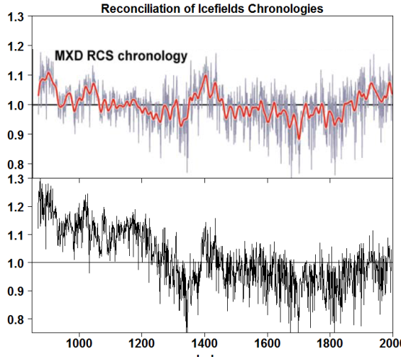
Figure 1. Top – MXD RCS chronology from Luckman and Wilson 2005 Figure 2; bottom – MXD RCS chronology calculated under alternative assumptions – see Figure 3 below.
I will use random effects statistical techniques both to analyse the data and to place prior analysis in a more formal statistical context. Because LW2005 coauthor Rob Wilson stands alone for civility in the paleoclimate world and because the present post is critical of past analysis, in some ways, I would have preferred to use another example. However, on the other hand, it is also possible that Rob will recognize that the techniques applied in the present post – techniques that are unfamiliar to dendros – can yield fresh and important insight into the data and will look at the Icefields data a little differently.
Although the article in consideration was published more than a decade ago, the analysis in today’s article was impossible until relatively recently, because coauthor Luckman withheld the relevant data for over a decade.
Background
In 1997, Brian Luckman (Luckman 1997) published a tree ring chronology from the Athabasca Glacier, Alberta area that was used in several contemporary multiproxy studies (Jones et al 1998; Crowley and Lowery 2000).
In the late 1990s and early 2000s, the data was updated and expanded. In 2005, Luckman and a former student well known to CA readers (Rob Wilson) combined data from the Athabasca Glacier location with data from near Peyto and Robson glaciers to form “regional chronologies” for both MXD (density) and RW (ring widths), settling on “RCS” and “standard” methods, respectively, though, as we will see below, the eventual “RCS” method was idiosyncratic. The MXD and RW chronologies were then used in a regression to calculate a temperature reconstruction, which, in turn, has been used in multiple subsequent multiproxy and/or multi-site studies, including the recent Wilson et al 2016 multi-site temperature reconstruction. reported in Luckman and Wilson (2005 ).
As is far too common in paleoclimate, Luckman did not archive his data when the article was published. Luckman also turned down/ignored requests for measurement data that I made many years ago. In May 2014, long after the original articles had faded from view, Luckman finally archived the underlying measurement data. (By coincidence, this was almost exactly the same time as the decades overdue archiving by Jacoby and D’Arrigo.) I didn’t notice this long overdue archiving at the time. However, during my re-examination of series used in Wilson et al 2016, I noticed that the long refused data for the Icefields sites had finally been archived, making the present assessment possible for the first time.
Unsurprisingly, there are some surprising results – if I may put it that way.
Today’s post will be limited to the MXD data; I hope to get to the RW data on another occasion. I’m looking first at the MXD data since CA readers will recall some recent assertions by specialists favoring MXD (density) data over RW (ring-width) data.
The MXD Data
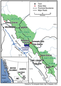
Because of the long delay between original publication (2005) and archiving (2014), I took particular care to try to ensure that the data in my present collation matches (at least as closely as possible) the data that was used in the original article. Figure 1 of Luckman and Wilson shows that data for the regional chronology came from three sites: Athabasca Glacier, Peyto Glacier and Robson Glacier.
Figure 2 of Luckman and Wilson showed core counts by year for four groups: Icefields living and “snags” (subfossil), Peyto living and snags from Peyto and Robson snags. 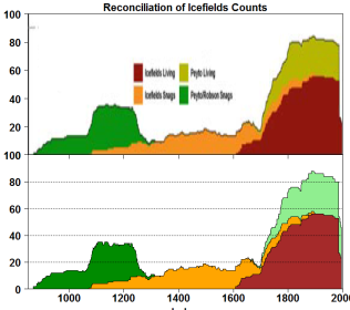
I was able to closely replicate LW2005 Figure 2 (See bottom panel at right) by collating the following six MXD datasets at the NOAA archive:
- three datasets from the Athabasca Glacier area (living: cana096x, sampled in 1983, and cana430x, sampled in 1994 and archived in 2014; subfossil: cana431x, archived in 2014.
- two datasets from Peyto Glacier area (living: cana097x, sampled in 1983; subfossil: cana445x, archived in 2014.
- one dataset from Robson Glacier area (subfossil: cana448x, archived in 2014).
There are two Athabasca Glacier MXD datasets at NOAA that were not used (cana170x, cana171x – both from Schweingruber.) My collation of the MXD data from the six sites into a “tidy” file (tidy, as defined in R usage) is at http://www.climateaudit.info/data/proxy/tree/wilson/2005/collated_icefields_mxd.csv.
RCS Chronology Variations
“Standard” (as opposed to “RCS”) tree ring chronologies fit a growth curve to each individual tree and then take an average of ratios (rather than residuals, though the effect is similar) for each year to form a “chronology”. As I’ve discussed from time to time, this is formally equivalent to the assignment of random effect to each tree. Since the trees have different life spans, this technique necessarily transfers variance from annual effects (the chronology) to inter-tree variance and effectively eliminates centennial variability – a phenomenon familiar to dendros (the “segment-length curse”) though they don’t explain it in the statistical terminology preferred at CA.
“RCS” methods are homemade attempts by dendros to mitigate this difficult problem. One common technique is to use single regional curve to “standardize” cores for juvenile growth , as, for example, in the Yamal regional chronology of Briffa 2000 or the Gulf of Alaska chronology of Wiles et al 2014. Luckman and Wilson 2005 briefly discussed use of a “single regional curve”, but dismissed it summarily on the grounds that it might “possibly introduc[e] bias in the earliest part of the reconstruction”:
Using a single, regional curve would inflate the final indexed values for the Peyto-Robson data, possibly introducing bias in the earliest part of the reconstruction.
I cannot help but comment that one seldom if ever hears corresponding concerns about inflation of final indexed values when the bias pertains to the latest part of the reconstruction. The results of an MXD RCS calculation using a single regional curve are illustrated in the bottom panel in Figure 1 above: it has a very “warm” medieval period. Perhaps this is the “bias” that concerned the authors of LW2005.
To implement a single regional curve RCS using a well-known statistical model, I fitted the data using the nls function of the nlme package (and then taking annual averages of the residuals). I used a negative exponential, as a Hugershoff function is not required here – in a Hugershoff fit, the coefficient is close to zero. The single curve model is:
fmnls=nls(x~ A + B* exp(-C*age),data=tree,start=c(A=50,B=30,C=.02))
To examine potential random effects from the three different sites, I used the lmer function of the lme4 package to concurrently estimate crossed random effects for (1) site and (2) year (as discussed in a prior post here ^). As in my prior discussion, I simplified the calculation by keeping the negative exponential coefficient C fixed (using the coefficient from the nls fit).
nm= lmer(x~ exp(-0.0030179 * age)+(1|site)+(1|yearf),data=tree)
While I have not exhaustively studied the matter, the chronology of random effects do not appear to be materially impacted by slight changes in this coefficient.
I also did a model in which I included one more crossed factor distinguishing between subfossil/living – as well as for site.
nm1= lmer(x~ exp(-0.0030179 * age)+(1|site)+(1|sf)+ (1|yearf),data=tree)
I am more than a little troubled about introducing a random effect for a subfossil/living distinction without evidence of a physical difference, because the introduction of such a factor will necessarily transfer variance from the chronology to the factor and, in the process, compromise the chronology – an issue that I will discuss further below.
The next figure shows the RCS chronologies resulting from each of these three statistical models: top – nls; middle – lmer with a random effects for year and site; bottom – lmer with random effects for year, site and subfossil/living. In each of the above three cases, there is a pronounced MWP period, most pronounced in the nls case (see discussion in caption), but evident in all three. Each has a very different medieval-modern relationship as compared with the reported LW2005 chronology.
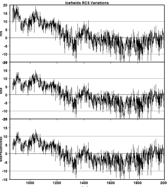
Figure 3. RCS chronology variations: top – nls fit; middle – lmer fit with random factors for year and site; bottom – lmer fit with random factors for year, site and living/subfossil. As we previously observed with the Polar Urals MXD chronologies, the lmer chronologies damp chronology values when measurements are sparse – observable here in the earliest values. When measurements are sparse, the lmer method keeps some of the variance with the residuals.
The LW2005 RCS Chronology
So how did Luckman and Wilson arrive at their RCS chronology without an MWP?
Rather than calculating a random effect for each site or crossed random effects for site and living/subfossil (as the two examples above), they divided the data into three somewhat idiosyncratic groups:
- living trees (combining Athabasca and Peyto);
- Icefields/Athabasca snags (subfossil); and,
- a combination of Peyto and Robson snags.
As an experiment, I calculated a chronology using lmer with crossed factors for (1) year, and (2) the three LW2005 groups. This did indeed yield a chronology that no longer had the high medieval values of the other RCS choices shown above.

Figure 3. Top – MXD RCS chronology from Luckman and Wilson 2005 Figure 2; bottom- lmer chronology of annual effects, using LW2005 grouping as a random effect. As in other examples, the lmer technique damps early values when measurements are sparse. The model used is:
nm3= lmer(x~ exp(-0.0030179 * age)+(1|alias)+ (1|yearf),data=tree).
However, there is a serious hidden cost to the grouping selected in LW2005.
In a grouped RCS calculation, each of the three groups is effectively centered at the same mean, even though their temporal coverage is entirely different. The average dates of the Peyto/Robson snags, Icefields snags and living trees are 1109, 1484 and 1855 respectively. The average date of the Peyto and Robson subfossil material is in the heart of the medieval period, while the average date of the living tree datasets is in the very cold 19th century. Nonetheless, the LW2005 grouping centers all three groups at the same level, as can be seen in the table below showing the average ring width for each group, together with the random effect of the above statistical model: after subtraction of the random effect for each group, the group values become virtually identical:
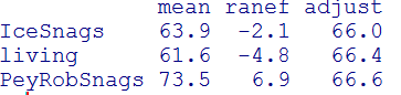
By choosing to separately standardize living and medieval data (Peyto/Robson subfossil), the possibility of drawing conclusions on medieval-modern data is rendered impossible, in effect defeating the purpose of the RCS calculation.
I think that the problem is neatly illustrated by the next diagram, which shows average annual MXD values from the two Peyto datasets (living and subfossil). In a single regional curve – or even when a single factor is assigned to the Peyto site – the high medieval MXD values yield high values in a chronology. However, if Peyto subfossil/snags are treated as a different site than Peyto living (as, effectively in LW2005) the high MXD values are allocated as a random effect of the site and cancelled out of the chronology.

Figure 4. Annual average MXD values from Peyto glacier data, combining data on living trees and snags.
LW2005 purported to justify a technique that cancelled the high medieval values on the basis that this technique permitted the “better assessment of potential bias from the RCS method”:
To address the potential occurrence of differing ‘populations’ within the MXD data, the MXD series were divided into three groups, to allow better assessment of potential bias from the RCS method (Table 4).
However, I fail to see how the LW2005 permutation allowed a “better assessment of potential bias”. Even if this permutation proved better in some sense than other potential permutations (including the ones presented in this post), LW2005 merely presented this result as fait accompli, rather than as a measured recommendation following analysis of alternatives. To actually carry out such an “assessment”, one would need to examine results from other plausible groupings, such as those presented above – all of which had pronounced MWPs – and explain precisely why the grouping that happened to eliminate the MWP was “better” on a criterion more meaningful than a Calvinball elimination of high MWP values.
Conclusion
The RCS technique used in the LW2005 MXD chronology eliminated high medieval values as a tautology of their method, not as a property of the data. The Icefields data provides equal (or greater) justification for MXD RCS chronologies with elevated medieval values.
As I work through these examples, I am increasingly convinced that a statistical model using crossed random effects for site and for year provides a relatively rational basis for accommodating site inhomogeneity without sacrificing “low frequency” variability. It certainly seems more effective in each of the recent examples. This does not mean that the chronology of annual effects is necessarily a temperature “proxy” – only that such a chronology is a better estimate of annual effects (which may be due to temperature, precipitation, insects, fire etc.)
However, the analysis of today’s post was impossible until recently because coauthor Luckman withheld relevant measurement data for over a decade. One of the retorts to the present analysis will undoubtedly be that I’m wasting my time dissecting a decade-old paper, because the field has “moved on” (all too often to still unarchived data (e.g. most of the component series of Wilson et al 2016) which, if the past is any guide, may not be available for another decade.
But while new datasets have arisen during this period and while “RCS” chronologies have become fashionable among dendroclimatologists, dendroclimatologists have limited understanding of the statistical issues involved in the construction of a chronology, and, in the absence of a rational statistical theory for “RCS” chronologies, the construction of such chronologies all too often seems to become prone to a peculiar form of Calvinball in which arbitrary decisions invariably seem to inflate modern values relative to medieval values (as appears to have taken place in the present and other cases.)
References:
Luckman et al 1997. Tree-ring based reconstruction of summer temperatures at the Columbia Icefield, Alberta, Canada, AD 1073-1983. The Holocene.
Luckman and Wilson 2005. Summer temperatures in the Canadian Rockies during the last millennium: a revised record. Climate Dynamics pdf.
Wilson et al 2016. Last millennium northern hemisphere summer temperatures from tree rings: Part I: The long term context. QSR. pdf


78 Comments
Steve, I’m overjoyed to see your continued deconstruction and disambiguation of the tree ring data.
I was saddened but not at all surprised by this statement:
The tragedy of modern climate science is that this kind of scandalous scientific malfeasance goes not only entirely unpunished, but is completely ignored by the overwhelming majority of mainstream climate scientists. Gotta say, it angrifies my blood. People tell me all the time that I’m too passionate about this kind of scientifically criminal behavior.
The taxpaying public funds these charming fellows to go adventure in the wild and secure important scientific data, and they treat it as if it were their own. Disgraceful and shameful. Me too passionate? I say that people are not passionate enough about this underhanded, deceptive withholding of scientific information.
Except Canadians, I have it on good authority that they never sweat unless there’s emotional attachment. But for the rest … where is the richly deserved outrage?
But I digress. Good stuff, and fascinating. I gotta learn more about “random effects statistical techniques”, where might I start my further education?
My best to you,
w.
“Angrifies” me as well. This withholding stops science dead in its tracks, and on the taxpayers’s dime yet! Well, it doesn’t really make any difference whose dime it is on, it is still “anti-science”, to purloin a popular phrase of the day. Karl Whose-name-is-on-notice-for-being-banned-here would also have a fit. If we all get blase about this practice, then the bad guys win.
Makes me wonder why they would have archived the data a full 10 years later. After waiting a full 10 years, you gotta wonder what is the reason for the sudden change. Seems as though there must have been some new reason that either suddenly appeared in the 10th year or gradually grew over time that motivated the act. Is is so that the scientists can truthfully but misleadingly claim they archive all data (omitting the time lag in their claims)? Is it because they are seeing that mother nature and newer studies are diverging from the older studies and there now needs to be clear evidence of the reason for the divergence? Is it because 10 years is long enough to feel safe enough that the Steve M’s of the world will likely not pick apart the study, as was done here only by chance?
Steve, many thanks for a very clear explanation of what appear to be appalling methods used in the LW2005 paper, and demonstration of their effects.
I second Willis’s comments.
Steve McIntyre,
The subfossil MXD are presumably difficult to use because we observe a loss of density from the outer rings. The very high medieval values you get could possibly come from this behavior.
Steve: subfossil MXD series are used all the time in reconstructions without this caveat being provided. Do you have a basis for the above assertion or are you just speculating?
Steve McIntyre,
When trying to eliminate the selection bias, I got the same effect with the data of Briffa 2013.
Similar problem for Jeff Id:
One can observe the phenomenon of density loss in this graph:

It is no longer representative after 200 years because there are too few samples.
The purple line represents the average of subfossil.
I didn’t understand your previous comment which IMO was ill-phrased. When you talked about “loss” of density in subfossil trees, I thought that you were talking about some sort of post-deposition change, but your sources refer to garden variety decline of density with age of a tree, a phenomenon very well known to dendros and the reason for “standardization”. If that’s what you’re talking about, it’s baby food.
Jeff Id and Roman didn’t purport to have discovered this phenomenon, but were reflecting, as I am, on a more rational way of developing a chronology when data is impacted by juvenile growth. I don’t recall Jeff Id’s post though it’s a topic that interests me. I may have missed it at the time. Now that it’s been drawn to my attention, I’ll try to reconcile my methods to what Jeff and Roman were doing. At a quick look, it seems similar to regional curve RCS, but I’ll have to parse it.
Steve McIntytre,
I’m not talking about the well-known variation in density with age, but of the loss of maximum density of dead trees from the outer rings. This is what show the graph.
OK, I see what concerns you. It isn’t what is at issue in the Jeff Id post, which is an interesting reference.
However, I don’t think that a few readings in outer rings won’t have a material impact on the curves.
This issue is only slightly related to the statistical issues of this post. As a general editorial policy, I discourage the coatracking of general issues when a thread is specific. The question of erosion of density from outer rings of dead trees is duly noted and I’ll try to look at it at some future date.
Steve McIntyre,
I mentioned this problem because I think it is the cause of the high medieval values you get (as for Jeff). When samples become few, the slope of densities can dictate the form of the reconstruction.
Are you feeling alright this morning, Steve?
davideisenstadt,
I can only repeat what I have already said, unusable in the current state.
For living trees, I let you judge: https://climateaudit.org/2016/02/08/a-return-to-polar-urals-wilson-et-al-2016/#comment-767075
I agree that phi’s comment was vague/misleading tho well-intentioned. The decline of density as trees age is so well known that it never occurred to me that that was the phenomenon that he had in mind. I thought that he was discussing some sort of post-death decline not discussed in the literature.
I’ve posted a reply and removed some comments which are not relevant once one figures out what phi actually meant.
I find it much easier to accept the claim of a 5+ sigma detection of gravity waves (producing a 1/1000 shift in an atom’s nucleus) than dendro claims of “warmer” or “cooler” based on their idiosyncratic collections of tree cores — to say nothing of claims for tenth of a degree temperature anomaly differences centuries ago.
Unfortunately, I also believe the earth’s temperature, current and past, is the more important research project.
Thanks for presenting a critique without criticism, in that it invites a response without being hostile. It invites people to try to reach an understanding of the genuinely difficult issues.It would be good if the dendro guys could respond in kind, because there is a lot to debate in this area.
Thanks again. Nit: Athabaska? I thought it was Athabasca….
Steve: both spellings occur, but Athabasca is the more common. I’ll edit.
I was really very surprised when such high medieval values were produced using common RCS methods. There obviously isn’t any hint of such tendencies in the academic literature.
The Icefields series was very influential in the reconstructions which were popular when I first started e.g. Jones et al 1998; Crowley and Lowery 2000. – both of which would be materially impacted by an Icefields version with a high MWP (together with other problematic series e.g. from Polar Urals, Yamal and, of course, the Tornetrask bodge.
It would have been nice to have had this data 10 years ago.
‘Calvinball’ is certainly the most apt of metaphors to describe your recent series of posts. MWP elimination by methodological tautology. Just when we thought we had seen everything.
For those few who are unaware of “Calvinball”:
http://www.picpak.net/calvin/calvinball
Hope the link worked!
Those few = 97% of the world’s population. Thanks for the link.
I think the UK equivalent is Mornington Crescent.
https://en.wikipedia.org/wiki/Mornington_Crescent_(game)
Steve – in the spirit of your comment wrt Rob Wilson, is this line of work worthy of a (joint) paper? If a climate publication won’t take it, would a stats journal publish it as it an example of an application of an alternative technique to an established subject area, one which yields novel results?
Steve and others have been urging the climate science warmist community for years to jointly work with competent statisticians in doing their work, with whatever data they are using. I doubt seriously that Wilson, in spite of his willingness, on occasion, to participate on this blog, would be willing to work with Steve on these studies. I will not speculate on his motives for this probable reluctance, but for the majority of these guys the simple facts are that they know that if they did use competent statisticians their results would not be to their liking and probably would not get published in their pet journals.
In addition, it would probably mean that they could no longer keep their data in a closet for years.
PhilH
Steve: Rob gets vile abuse within the dendro community for even discussing these issues. We had lunch at AGU some years ago at a cafe near the Moscone Center. Someone from CRU spotted us and couldn’t wait to report Rob’s transgression to Phil Jones. Rob was junior and itinerant enough that he was vulnerable to the climategaters. Some years ago, I was invited to give a presentation at a dendro conference in Finland, at which time I planned to discuss my statistical ideas. But climategate occurred and my invitation was withdrawn as the dendro community circled the wagons around bodging and hide-the-decline.
Mr. McIntyre–
OT: A bit ago I went to access “Acronyms” under “Links”, above, and got only the message “Not Available”. Is this something you can fix?
Was wondering about that too. Appreciate if it could be fixed…
The “wikispot.org” site which held the acronyms page has apparently shut down.
Archive of the acronyms page may be found here.
HaroldW–
Thank you!
Och – I really tried to get to this today but teaching must come first this week. Steve – I am not surprised you picked up on this issue as it is certainly tempting if you want to “fish” for a warmer medieval period – not that I am accusing you of this . However, the Peyto and Robson data do not reflect the same location conditions as the data from Sunwapta/Athabasca and so there are unique ecological issues that affect tree growth which will influence the whole approach to RCS and also I think your random effects approach. It is for this reason we treated these data as their own group. This is simply a more conservative approach – i.e. 3 RCS groups rather than a single one. A single RCS curve in this case would lead to potential bias – i.e. elevated values in the Medieval – as you have found. This is a standard approach in RCS when working with heterogeneous TR data-sets. Figure 7a in the Appendix of L+W05 clearly shows the higher raw density values for the Peyto and Robson data. Figure 7c also shows that there is an offset between the Icefield snags and Peyto/Robson RCS indexed chronologies. I did toy with the idea at the time of calculating the mean difference between the two chronology sub-sets and “lifting” the medieval values accordingly, but it would have been (and still would be) difficult to justify. Hence the current published version is a conservative approach using a 3 RCS group approach. This captures more low frequency variability than using single series data adaptive approaches (see Luckman et al. 1997), but certainly by having the medieval data as their own group does potentially depress the mean index values for that period to the long-term mean. To be honest, if I did the analysis today, I would not do it any differently although I might play around with an ensemble approach to derive a range of versions (i.e. yours would be one “warm” extreme end member). What is really needed here to resolve this issue is to go back find/take more samples? Easier said than done alas.
Finally, just to highlight the heterogeneity of the data as a function of location, plot the raw ring-width data in a similar way as you have done – whether as a non-detrended mean or going through the random effects approach. You will find that medieval values are LOWER which is not very logical if the period is so much warmer.
Rob,
I understand that you responded quickly, but you didn’t correctly understand the form of the analysis. In doing so, you’ve incorrectly presumed that I’ve neglected obvious points.
I analysed multiple variations, only of which was a single regional curve. I also analyzed a variation in which a random effect was assigned to each site and crossed random effects, one to site and one to subfossil.
You say:
I’ve consistently criticized the use of a single regional curve when there is inhomogeneity between sites, as one must assume e.g. my critique of Briffa’s Yamal chronology and more recently, my commentary on Gulf of Alaska. However, it strikes me that dendros are much more alert to presumed “bias” when it impacts medieval values and tend to shut their eyes when it contributes to high recent values – as in some of the curves used in Wilson et al 2016.
In the post, I showed several calculations, commenting most extensively on calculations in which a random effect was assigned to each site.
You say that the use of three groups is “more conservative”. Note that my calculation with a random effect for each site also uses three groups and by your criteria is just as “conservative”. However, the term “conservative” is not a helpful statistical term as it lacks a precise meaning. Worse, in the present context, as I pointed out in my post, your methodology ensured that medieval and modern levels are more or less equivalent through your construction: as I observed in my post, it is tautological from your method. To describe such a method as more or less “conservative” is meaningless. In saying this, I am not excluding the possibility that one could arrive at similar results using a non-tautological method, only that your results employed this defective method.
I had not read your post. My comment was just a quick clarification of our decision process in 2004.
Rob, you say:
Too wishy washy. It necessarily depresses the mean index value through the math.
That’s not to say that there might not be valid grounds to be suspicious of the high values, but you didn’t present the case either way as your methodology foreclosed any discussion of this issue through its methodology.
Rob, thank you for your comments, always good to hear from you.
It seems to me that this is the same issue involved in the Berkeley Earth “scalpel” method for dealing with temperature records. In that method, as the name suggests, when there is an “empirically determined breakpoint” or station move or a gap in a station record (as in Figure 4), that record is cut into two records.
As Steve points out, if you cut the record in two, you lose all of the long-term relationship between the two halves. Whether the start of the record was higher or lower than the end of the record, once you cut it into two records, it all goes flat.
If I understand what Steve is saying, this is what he means by “tautological”—any record that you cut in that manner will end up flat by definition. It is inherent in the chosen method.
Finally, you say:
I was curious how you determined that warm Medieval temperatures are a “potential bias”, particularly on a planet where such a generally warmer historical period is revealed in lots of proxy, observational, and anecdotal datasets …
Best regards,
w.
PS—I got into an internet bunfight the other day where I got ragged on for describing you as “one of the good guys” … and I still hold to that description.
Steve: I’d prefer that commenters not discuss Berkeley splicing (tho I am sympathetic to the point.)
Rob says:
I carried out the calculation on RW data that you recommended, using an identical technique as the one that I had used on MXD data. I obtained high values in the medieval period – opposite to your assertion. (If one does a simplistic average of raw values or single regional curve, one gets low medieval values, but this does not properly account for inter-site variance.)
Figure 1. RW chronology of annual random effects from a dataset collated from the following seven Icefields, Alberta RW dsets: “cana096” “cana430” “cana439” “cana097” “cana434” “cana445” “cana448” (after ensuring that units were compatible), using the same lmer technique: crossed random effects for site and year. Values shown when 10 or more cores. Horizontal line shows pre-1440 average.
In this example, there was a wide variety of ring widths, as evidenced by the following wide range of site random effects, and the wideness is a severe test of the random effects technique:

Rob, I hadn’t argued that the data proves that the MWP was “so much warmer”. I have criticized the statistical work in peer reviewed literature, but have not advanced my own interpretation. In doing so, I’ve observed that plausible – and indeed preferable – techniques yield high medieval values of the chronology.
I am confused by the dataset IDs. Steve’s comment here lists 7: all “cana” prefix with suffixes 096, 097, 430, 434, 439, 445 and 448. Steve’s original post had 6 datasets (The MXD Data) with suffixes 096, 097, 430, 431, 445 and 448. So where did suffixes 434 and 439 come from and where did 431 go?
Steve: the original analysis was on MXD data. I then did a similar analysis on RW data – the dsets for which are slightly different.
too late to look at this Steve, but it seems rather illogical for the Robson/Peyto data with such low growth rates to be so heavily “uplifted” in your random effects plot.
Will try and look at this at the weekend
Steve: I did the run quickly. I’ll post up a script to replicate the results.
Looking separately at the Peyto site data – I’; post a graphic up later, I agree with ob’s comment that the subfossil trees are inhomogeneous with the living trees. The downside is that, if the subfossil trees at a site are inhomogeneous with the living trees, then, as I had observed, the ability to compare periods is compromised. The methodological problem – which is what I have been reflecting on – is that practitioners seem alert to such inhomogeneity when the effect is a higher MWP, as here, but less alert when the inhomogeneity leads to elevated modern values.
Steve: There were no local living trees at Robson to check for homogeneity or use for calibration. That I data comes (arbitrarily?) from Peyto.
Steve: the subfossil trees at Yamal do not necessarily come from the same locations as the living trees. Why do dendros worry about homogeneity in one location and not the other?
At sites where sub-fossil wood from the MWP can be collected, but no living trees exist, why don’t dendros draw the obvious conclusion: the MWP was warmer than the CWP? For how many decades can a site be at least as warm in the CWP as it was during the MWP and still have no living trees where trees grew during the MWP?
Steve: changing treelines have been something that I’ve been interested as the evidence seems readily interpretable. As an AR4 reviewer, I asked them to comment on treeline changes, but IPCC rejected the idea. Their view is that present day tree lines are not in equilibrium with present temperatures and will gain more altitude. I think that the better way of handling the situation would be to review the data and comment on the expected equilibrium line.
Rob: Assuming I understand correctly, you need samples at every site from the instrumental period to calibrate your reconstruction of earlier temperatures. You have samples for the CMP and LIA from the Icefields site, but few for the MWP. The Peyto site provided samples from both the CWP and the MWP, but none for the LIA. Finally, the Robson site has samples only from the MWP, and therefore must be calibrated via one of the other two sites with samples from the instrumental period. Why was the more distant Peyto site chosen? Given the absence of samples from the CWP and the differences between these sites, why do we believe the Robson samples contribute anything to our understanding of the MWP in this area? If the other two sites provided an adequate chronology, why include Robson?
1,000 years ago, Glacier Bay was a grassy valley with a salmon-rich river running through it. By 1794 it had been scoured by a massive glacier and was covered in 4,000 feet of ice. By 1915 it was a 65-mile-long bay.
Since the glacier began its retreat, there’s been isostatic rebound of as much as 5.7 meters, and, with the current rise of up to 30 mm/year continuing, the upper bay might yet become a valley with a river running through it.
Meanwhile, continued retreat of Mendenhall glacier to the south is exposing 1,000 year old forest.
Would it not be odd if dendrochronologies did NOT show warmer climate 1,000 years ago?
Verdeviewer: Unfortunately, we can’t learn anything reliable about the relationship between MWP and CWP temperatures when retreating glaciers expose trees that grew during the MWP. It takes many decades for the terminus of a glacier to come into equilibrium with local temperature and even longer for trees to begin to grow. Sure, we know that the MWP was warmer, but we don’t know if it was warmer than the CWP in 1900, 1950, or 2000. There is a big difference between this three. The big advantage is they contain iquantitative nformation about a specific year (or several years).
At several (most?) TR sites, sub fossil wood from the MWP has been collected north or above the current tree line. Tamales, for example. In this study, only snags were collected from the Robson site, suggesting that trees don’t grow there today. How long after the restoration of MWP warmth will it take for trees to return to the Robson site?
shouldn’t the question be:
“How long after the LIA will it take for trees to return to the Robson site?”
David: The density of latewood of trees at a particular location contains a signal for the Average JJA temperature of a particular year, say 10.0 degC in 1300. To the north of that location or higher in elevation, the tree line has been retreating southward and terminus of a nearby glacier has been advancing. Those processes requires decades reach a new equilibrium in response to LIA cooling. Now skip ahead to 1950, when latewood density again is consistent with an average summer temperature of 10.0 degC. The tree line and glacier terminus won’t have returned to the equilibrium position of about 1300, because this response takes decades. Now skip ahead to 2000. The maximum latewood density is consistent with an average summer temperature of 11.0 degC. Should the tree line be north or south of the position in 1300? Should the glacial terminus be above or below the position in 1300? If the locations in 1300 haven’t been recovered by 2000, we can say that the MWP was warmer than the CWP at some point during the twentieth century, but we can’t say that it was warmer during the 1960’s. Only annual signals like MXD can provide a comparison between the 1300s and the 1960s – ior it would if there weren’t so many options for processing MXD signals.
the question isnt whether tree rings provide a reliable temperature signal…sometimes they do; sometimes they dont.
geez.
David: If the temperature reconstruction has a properly calculated confidence interval, the width of the confidence interval should increase when more sites show poor correlation with temperature during the instrumental period. When your analysis starts by cherry-picking the sites with the best correlation, the confidence interval shrinks inappropriately. I suspect that your “some trees do and some trees don’t” isn’t a fundament problem that can’t be addressed with a proper confidence interval. The more noise in the signal; the wider the confidence interval.
Frank,
Certainly. But there is a big problem. The high frequency signal is generally excellent and the low frequency signal excecrable.
The Australasian temperature reconstruction authored by Gergis attempted to use high frequency correlations (detrended) for post facto selection of proxies and found that the correlations were not as good as the low frequency when they learned that they had forgotten to detrend.
High frequency correlations are what some dendros evidently feel is the more rigorous correlation but few ever get around to using it. Actually there is a mighty dilemma here. It is the low frequency trend that is important in temperature reconstructions that are after all produced to look at trends. Post fact selection becomes even more off the mark because the low frequency “trends” in a highly autocorrelated proxy series are rather easy to match to another series trend which in this case is the instrumental record. In the high frequency domain it is not sufficient for the proxy to react in the correct direction to the prevailing temperature it also has to track the temperature change in a reasonably reliable portion.
As ancient settlements are given up by retreating ice, I’m sure studies of clo and R values (adjusted and normalized) will show it was much colder.
verdeviewer, your remark on the nature of the “snags” and their connection to phenomena like the retreat of the Mendenhall Glacier really puts this entire issue in perspective. If I understand you correctly, the real evidence of the LIA and a preceding warm period is simply the existence of the snags. This is not to discount the importance of analyzing the tree data correctly, and I really appreciate the links to the newly available data and the R scripts in this discussion. But we seem to be arguing about the number of angels on the head of a pin. It is emblematic of our current malaise that Obama would choose Mendenhall Glacier’s retreat as an example of the effects of AGW when the real story was the debris exposed at the bottom of the retreating glacier.
The column headings in the ‘icefields mxd.csv’ file are; id, year, age, rw, dset, yearf, site.
Is this correct?
This is pretty amazing. This would be like demeaning stock market data in up and down markets separately and then concluding the performance is the same.
Steve: pretty much.
SteveM and Rob Wilson, are the finished reconstruction data available for someone to look at and model the noise? I am always curious as to what a simulation of the modeled noise will look like – as in long term persistence or a high degree of auto correlation. High correlation of two trending series is not a task difficult to accomplish. In this case I do not recall whether the the detrended TR series and the detrended temperature series were correlated.
Actually the series I see for the Wilson reconstruction in this post would be easier to reconcile with high auto correlation noise or long term perristence.
Steve: yes. I’ll post up some scripts and include this.
Reblogged this on I Didn't Ask To Be a Blog.
This is the first reference I happened upon that just so happens to also show the same shape as Steve M’s curves above for the Athabasca area, this data being derived from lake sediments. Very much the same as above with a pronounce MWP and
cool LIA. See Figure 2 below. Just sayin’.
http://onlinelibrary.wiley.com/doi/10.1029/2008GL036125/full
Here is a script which collects previously collated icefields rw data for the 7 sites listed below and which calculates and plots the following chronologies:
1. mean value
2. residuals from nls model (single regional curve)
3. residual chronology from nlme model (curve for each site)
4. chronology of annual effects from lmer model with crossed random effects for year and for site.
The contrast between the cana096/cana097 and Peyto/Robson snag random effects is noticeably greater in the lmer model than in the nlme model (see annotation in script) resulting in a very different perspective on the data. I don’t have time right now to post up the figures produced in the script below, but they are a very interesting sequence. I’ve tried to make the script self-standing (though you need the lme4 and nlme packages in R).
I didn’t run this script to “fish” for high MWP values. I used my regular script for regional chronology with crossed effects to examine the RW data that Rob challenged me to reconcile. I’ve recommended crossed random effects as a statistical model long prior to this post and have consistently preferred this perspective on the data. In saying this, I’m not saying that chronologies so produced are “right” or that they can be used as temperature proxies, only that the procedure seems more rational to me than worse methods.
What, no 10-year waiting period?
I’ve learned that a basic assumption of linear regression consists in the residuals (data values minus modeled values) being distributed normally. Below I’ll try to attach a figure showing a QQ-Plot generated from the lme4 regression above. If the inclusion of the figure fails, the QQ-plot can be generated by calling “qqnorm(resid(nm));qqline(resid(nm))” in R after running Steves script (and after correcting for a few oversights therein).
I find it difficult to assess how much deviation from the normal line in a QQ-plot would be tolerable. Would it be tolerable, in this case? Could it be that the exponential deviation indicates a hidden variable not being accounted for by your model? I’ve tried a log transformation of the density values, but this does not really fix the problem.
In addition, when plotting resid(nm) ~ fitted(nm) the prominent wegde-like structure clearly indicates heteroscedastic variances, which lme4 does not handle correctly as the calculated standard errors will become unreliable.
As for random effects in general, I remember to have read a statement from D. Bates that the number of factor levels of a factor used as a random effect should be at least five, because else the attributed variance would grow unreasonably large. This does probably not affect the 1|dset effect (seven levels), but certainly would affect the 1|sf random effect within the “nm1” model, with “sf” having only two levels. Bates once suggested to model such a variable as a fixed effect instead.
The non-normality of the residuals is also present in your lmer model in the earlier post on “A Return to polar Urals: Wilson et al 2016”. After removing some huge outliers there, an prominent exponential deviation remains visible in the QQ-plot.
I also wondered why you did manually average over the repeated determinations (the cores) for the same tree when constructing the Wilson 2016 data set. If they did around five cores, one would get a measure for the overall coring precision by including 1|id as a random effect.
QQ-Plot of the “nm” model residuals:

yes, the residuals for RW can be very non-normal. On many occasions, I’ve described the many problems in trying to develop a tree ring chronology using statistical concepts and have noted that heteroskedasticity, non-normality and autocorrelation all are involved over and above the random effects.
The problem that I’m trying to highlight is that the construction of a tree ring chronology is a statistical model – a concept that is completely foreign to practitioners.
I’ve not asserted that there is any magic solution to the problem, only that this sort of modeling places the issues in the open. The issue that you point to is definitely one of them.
The lmer and nlme programs have options for heteroskedasticity and autocorrelation which I’ve experimented with from time to time in the past. I didn’t have much success getting these options to work on the relatively large tree ring datasets when I tried about six years ago but I was working with slower and smaller computers at the time. It would be worth revisiting.
However, the residuals from the MXD data modeled in the post (rather than the RW data in the comment) are reasonable normal:

Here’s a prior discussion of non-normality in tree rings from 10 years ago – my time flies: https://climateaudit.org/2005/09/11/log-normality-in-gotland/ with some qqnorm plots that I had done at the time.

Steve:
I know that I harp on this consistently, but I cannot understand just how one can reasonably expect to surmount the issues presented by a proxy data set that is heteroskedastic, isn’t normal, and exhibits a significant degree of autocorrelation, all along with the proxy being dependent on a slew of other unrelated variables.
Creating a model to account for variance in tree growth due to the age of the tree in question, as well as assumption related to consistency in fertilization, light wind and any other thing one can imagine is not sufficient to make chicken salad out of the pile of chicken feces that one is presented with.
In the end, the “signal” that one coaxes out such a data set is more a representation of the researchers’ predispositions than anything else.
The fundamental assumptions of statistical analysis that undergird the entire enterprise dont apply.
homaskedasticity? nah
Gaussian distribution? why?
Independence of individual observations? thats for pikers.
All of this in an attempt to create a proxy thats supposed to be accurate to within a fraction of a degree celsius?
That is to be used, after detrending removes any high frequency variance, to compare temperatures on a decadal scale?
All of this starting with a “calibration” and winnowing of data by looking at the instrumental record?
Why is it that no one cares to actually learn about the tools they are utilizing?
Steve: Obviously I’ve pointed out all of the above problems in tree ring data for many years. One of the main benefits of presenting tree ring chronologies in random effects terms is that it places these issues squarely before the reader in a concrete way. In a tree ring article where they use ad hoc recipes, all of these problems are hidden. As to why dendros have so little interest in the statisical foundations of their discipline, you’d have to ask them. I think that the reason is that the leading specialists don’t even understand the questions.
At Climate Audit, I and most CA readers that pay attention to this sort of thread are well aware of heteroskedasticity, autocorrelation, nonnormality etc. Thus, I’m not that interested in generalized complaining about such issues, since I know these problems. Also, the presence of heteroskedasticity, autocorrelation, nonnormality doesnt necessarily consign the data to nothingness either. Their impact may be important or it might not be. Also, purely as a crossword puzzle, I think that it’s an interesting exercise to try to get a functioning lmer, glmer or nlmer model which incorporates the various phenomena. I’ve done many experiments in which the models hang up or don’t converge. I think that there are some excellent projects for a grad student who is capable of opening up the hood of these techniques. In a younger body and mind, I’d have been able to do that but I’m not sure whether I can anymore.
Sorry for the generalized complaint.
Current practices are simply maddening to me.
It would be a good thing to have more data, from more trees.
It also might be a good idea to put monitors on the trees to measure the growth of the trees on a continuous basis, maybe a cuff wrapped around the trunk with transducers that would measure tension in the cuff caused by growth?
One could cuff an entire population of trees at a site, have the data collected and then one could analyze at one’s leisure.
It looks as if the “cana430” data set introduces most of the deviation in the QQ-plot. By excluding “cana430”, also excluding the outlying trees ‘H01-014′,’H01-015′,’H01-021′,’H9309W’,’H9424S’,’H9431W’,’HA5202′ and finally log-transforming the rcs values as in lmer(log(x+1)~h(age),…), the residuals look not far from normal to me. The MASS::boxcox function returned a optimum lambda near zero and hence a log transform is appropriate. The dampening effect of the log transformation also vanishes the wedge-like structure in xyplot(resid(nm) ~ fitted(nm)) which means that unequal variances are gone too. Interestingly, the time series of the yearf random effect then shows a prominent hump between the years 900 and 1300 and a positive trend since 1600, thus accentuating certain peculiarities by doing an inverse Mannian, so to speak. However, the numeric experiment shows me that the selection of proxies is very sensitive to the outcome. It would be interesting to know why the “cana430” data set behaves so differently.
Steve: Tweaked/inspired by your comment, I independently re-examined this data as well. We were on the same page as I used log(x+1) as well. I got a glmer model to work with family=gaussian(link=”log”). I did a standard plot of fitted versus observed, color coding the dsets and observed the same cana430 phenomenon – which I confirm and agree with. I’ll experiment with your suggestions as well today or tomorrow. The improvement in lmer and home computers since the last time that I experimented with these things (about 5 years ago) looks considerable. The datasets ought to be of interest to lmer specialists since they are large and have interesting properties.
Six cores in cana430 (“A78-S2” “A8201” “A8307” “A8317” “D8104” “D8107A”) are in different units than the others and need to be divided by 10. I’ll update my collation to reflect this.
I did this only because I was following the script that I had used for Urals and that’s what Briffa had done. But you’re right that this causes information degradation.
I also confess to having trouble with nlme and lmer syntax and gains in getting models to work are hard-won. One would like to do a model which also has random effects for tree within dset and core within tree, but it might prove tricky getting the syntax to work right. I’ll experiment when I get a chance.
With lmer, a random effect for the intercept of trees within data sets could be (1|dset/tree), assuming that the tree names are unique only within each particular data set, else (1|dset)+(1|tree) should do the same. Cores within trees would be (1|tree/core), assuming the data set contains at least some repeated measures for each particular core. I’m unsure how to fit the tree age in this context, possibly (1|age)+(1|tree/core/age) as the precision could vary along the tree rings, in particular also at the outer rings of fossil trees as “phi” has pointed out elsewhere in this thread. A comprehensive syntax list which often helped me can be found in section “Model specification” at http://glmm.wikidot.com/faq.
Wrt unequal variances, to my knowlegde “lmer” still does not support them — only the older and essentially unmaintained “lme” and “nlme” functions within the R package “nlme” do.
Alternatively, mixed effect models allowing for heteroscedastic variances and possibly correlated samples can also be coded within a bayesian framework using the packages “rjags” or “rstan” and so on. I’ve tried that in another context, but it’s currently much over my head to assess its validity. Hence I’d appreciate it very much to see it applied here.
Hugo: thanks for these comments and thoughts. To my knowledge, nlme doesnt have a reasonable syntax for crossed random effects – something that is essential in tree ring application. In the recent posts, I’ve treated age as a nonlinearfixed effect with a single random effect for site. I’ve also experimented with log(ringwidth) as a linear fixed effect with age, which has benefits. I’ve experimented with glmer methods and different families e.g. gaussian(link=”log”) but haven’t got anything to converge.
Stepping back, one of the modeling issues that is distinctive to tree rings is that they often have a second burst of growth release in which juvenile growth levels occur in an old tree. This obviously doesn’t model very easily. I don’t know how to do it.
Steve,
is there a known physiological reason for a second growth burst? Repeated flooding, for example? I’ve observed a second lilac bloom once in my lifetime, in late september shortly after a very large and very unusual flooding receded (which lasted for two weeks or so). If there is evidence for such an event, the second growth burst should affect whole sites or at least many trees of a particular site at a particular time period. If so, could one not fit a higher order polynomial to adjust for theses sites and time periods specifically?
Thinking about your dendro posts, I was pretty sure that forestry science should have made use of mixed-effect models since a long time. So, when I just did a g**gle scholar search on forestry and mixed-effect models, I wasn’t much suprised that these models are actually applied in context of tree growth models all over the world. Not being able to immediately grasp the information offered there, I’d still bet that realistic predictions based on physiological models in forestry are of similar economic importance as are models predicting fish populations or diligent prospection models in the mining industry.
SteveM, thanks for the links and script to the processed data being discussed here. I will look at in the near future. In the meantime I found a TR reconstruction series from Luckman here:
http://www1.ncdc.noaa.gov/pub/data/paleo/reconstructions/pages2k/namerica2k/nam-tr_47-cana356-1200-1987.txt
I wanted to first assume that the series is merely red and white noise and then model the series based on that assumption and see what simulations would look like when compared back to the original series. I attempted both ARMA and ARFIMA models and found that an excellent fit good could be found for the Luckman series with ar1= 0.8967 and ma1=-0.4708 with a standard deviation for the ARMA residuals of 0.72. The best fit ARFIMA model had d=0 implying that the fit could be made without considering long term persistence.
The graphs linked below show the original series with 3 simulations below it. The difference in the 2 multi-framed graphs is the spline smooth used for smoothing the data was different. Notice that the simulations look much like the original series in the undulations and including some rather lengthy ones. If indeed the TR series are primarily noise of this nature it is easy to see where a post fact searcher would have fertile grounds for finding a temperature correlation – given that temperature and the TR series are both trending.
Can we pls have labelled axes?
Infrequent users can’t assume when the MWP was –
Was it 950 to 1250 AD?
Or 750 to 1050 years before present?
Thanks Geoff.
Phi:
Your graphic implies that the sample population drops below 10(!) 270 years or so ago..
to less than20 200 years ago.
do your really think anything of value can be inferred from the tree ring density of say, 15 tree rings in one spot on earth 270 years ago?
15 effing trees?
David,
These are just subfossil of one site. Years of outermost rings are spread from the thirteenth to the nineteenth century.
One sees especially the density loss from the outside. This probably means that the RCS method is useless and only introduces noise in the reconstructions.
the samples from one site are combined into a time series…in this case the time series is comprised of less than 20 samples for a good portion of the period in question.
My query remains…just what inferences do you think are appropriate to draw from a sample of less than 20 trees?
Note that the proper term is more likely d0 – l * e ^ -kn. This should give a good indication of the physical phenomenon involved.
Selle?
I don’t understand the process of archiving data. How/where does this happen? Is it readily available to the public? Any idea why Luckman would archive the dara when he did?
Jason, the main archive of paleoclimate data is the NOAA repository here. It is open to anyone and is a huge resource. As to Luckman … I know nothing.
w.
Somewhat off topic but I understand the Athabaska Glacier continues to shrink but as a consequence has revealed tree stumps that shoe there must have been some serious global warming from all those caveman fires in the past.
One Trackback
[…] https://climateaudit.org/2016/02/15/disappearing-the-mwp-at-icefields-alberta/ […]