Yesterday, I posted up a collation of Juckes’ reply to Willis’ comments. Today I’ll post up a collation of his response to my comments. The exchange is here , but, for some reason, this url hangs up for me and you might prefer to start here and follow the links. My comments covered some of the same ground as Willis – see the second half comments) but spent more time rebutting various specific allegations of “error” and “omissions” – errors that neither the NAS Panel nor Wegman identified. As you will see, Juckes is completely unresponsive to my detailed response to each allegation of “error” and/or “omission”. Instead, he merely stated ” We are concerned with the temperature reconstruction, not with the principal components themselves. Now that the code used in MM2005 has been made available some aspects of the calculation are clearer” and re-iterating this mantra as a response to each detailed rebuttal.
I apologize for not showing different colors; I don’t know how to do this in Word Press. So here’s how the layers are distinguished:
– the original Comment at CPD is in ordinary blog font;
– the Juckes et al response is in block quote
– if I make a current editorial comment, it is in italics.
I am dividing this review in two parts- one part dealing with section 3 in which our work
is criticized and one part dealing with section 4, the Union Reconstruction.
1. Juckes et al allege that our analyses contain a variety of errors, but do not cite or consider
the following relevant literature: the reports of the U.S. National Research Council
panel on Surface Temperature Reconstructions [North et al 2006 or the ”¬ÅNRC Panel”¬?]
and of the Chairman of the U.S. National Academy of Sciences Committee on Theoretical
and Applied Statistics and associates [Wegman et al 2006], or the exchange in
GRL between Huybers and ourselves (Huybers 2005; McIntyre and McKitrick 2005d –
Reply to Huybers).
2. Wegman et al concluded that our criticisms were ”¬Åvalid and compelling”¬?. The NRC
Panel specifically endorsed our key criticisms: of the MBH principal components
method (p.85, 106), of reliance on bristlecone pines as an essential proxy (50,106,
107); of inappropriate estimation of confidence intervals (107); of the failure of MBH
verification r2 statistic (91,105). It is really quite amazing that Juckes et al have ventured
into this controversy without any consideration or rebuttal of these relevant authorities.
Para 1: We allege there are serious flaws in McIntyre and McKitrick (2003, EE) and
McIntyre and McKitrick (2005, EE). We do not say that every statement in these papers
is false and the fact that some statements in those papers are indeed true does not
have any bearing on the the assertion that there are serious errors.Para 2: We are reviewing peer reviewed literature and are primarily interested in estimating
the temperature of the past millenium. Prof. Wegman”¬’¢s views on who Prof.
Mann might have talked and his survey of who has written papers with whom are very
interesting, but not on the topic of our review.
One of the guidelines to reviewers at Climatic Change is that articles have to discuss relevant up-to-date literature. This is mandatory. Obviously the NAS/NRC Panel report and the Wegman report qualify. The Huybers exchange was published in GRL in 2005 and covers the issue of covariance and correlation matrices (standardization) where Juckes et al throw stones. I can’t see what Juckes et al accomplish with such an insolent response.
3. In MM2005a-b, we illustrated the difference between the MBH PC1 and the PC1 from
a principal components analysis using covariance matrices, but also discussed results
using correlation matrices – a procedure which is exactly equivalent to dividing by the
standard deviation. In our Reply to Huybers, not discussed by Juckes et al, we gave a
comprehensive discussion of standardization issues in the context of the North American
tree ring network, illustrating PC series under a variety of standardization methods,
including the method said by Juckes et al to have been ”¬Åomitted”¬?. See recent online
discussion at http://www.climateaudit.org/?p=929. http://www.climateaudit.org/?p=928
http://www.climateaudit.org/?p=893
[especially the exhanges in
Para 3: We are concerned with the temperature reconstruction, not with the principal
components themselves. Now that the code used in MM2005 has been made available
some aspects of the calculation are clearer.
Well, it’s all very well to be “concerned with the temperature reconstruction, not with the principal components themselves”. But the allegations of “error” and “omission” pertain to the principal components. This was discussed with Juckes on this thread . Following my post, Pat Frank of Stanford also questioned Juckes’ failure to consider the Huybers exchange. For reference, here is a figure from that article showing the PC1 under a variety of standardization methods.

From McIntyre and McKitrick, 2005c (GRL).
In the face of this obviously comprehensive discussion of normalization issues, Juckes then accused us of failing to discuss normalisation in our earlier E&E article:
The other as yet unanswered question concerns why the importance of this choice of normalisation was not discussed in McIntyre and McKitrick (2005, Energy and Environment), given the dependence of the results on this choice.
I gave a detailed reply to this pointing out that our E&E 2005 article contained a specific discussion of the difference in results between using correlation and covariance matrices and that these were equivalent to results with and without division by the standard deviation (the normalization called for by Juckes although this is not a methodological decision for which he was able to provide technical support for from a third-party statistical text. Juckes then lamely said that he had “missed” this:
Re 21: Sorry I missed the fact that you had given an answer to some points on a later page.”
Well, if Juckes et al wants to accuse us of “serious errors” and “omissions”, it’s not good enough to simply “miss” such facts. It seems a bit reckless for Juckes et al to continue these allegations, given their present knowledge.
The other issue, discussed before, is that Juckes implies here that the code was unavailable, even though later on in his response, he admits that it was available. The discussion of covariance and correlation matrices (leading to the Huybers exchange) was based on the code archived at GRL in Jan 2005. Huybers consulted this code and had no difficulty in determining what we did. Huybers’ own code is at his website. The code for our 2005 E&E article was available on or before May 2005 as it was referenced by Wahl and Ammann at that time. The original objective of the code was to illustrate calculations. The EE code contained some references to my own computer directory and wasn’t fully turnkey and it was modified to be turnkey at a later date – without affecting any of the calculations.
So Juckes completely failed to support his allegation that we had “omitted” consideration of results with correlation PCs (division by standard deviation/ “full” normalization).
4. In our Reply to Huybers, we observed that tree ring networks were in common dimensionless
units and that statistical authorities (see references therein) recommended PC
analysis using a covariance matrix in such cases. We are unaware of any general purpose
statistical text recommending use of a correlation matrix in such circumstances
and Juckes et al did not cite any. We have never assumed that any PC
methodology could extract a temperature index from the grab-bag assortment of North
American tree ring chronologies and stated that the onus was on the proponent of any
methodology to establish the validity of the resulting series as a temperature proxy.
The NRC Panel (p. 87) considered this issue and stated that, ”¬Åin this case, argument
can be made for using the variables without further normalization”¬? and, in effect, endorsed
our position that the methodology needed to be proved from ”¬Åscientific”¬? (rather
than a priori statistical) considerations. Obviously, this discussion should have been
considered by Juckes et al.
Para 4: The units are dimenionless, but not common.
Again, Juckes answer is simply unresponsive. The tree ring chronologies in the North American tree ring network, which is primarily in question, were calculated by dividing ring widths for each tree by a fitted curve (a spline or negative exponential) to make dimensionless ratios and then averaging for each year. This is done for different sites. The resulting networks are not denominated in mm or g/cc, but in ratios. They are common dimensionless units. Juckes provides no citation or reference to justify whatever claim he is trying to make here.
5. Furthermore, even before the discussion in Reply to Huybers, we had previously discussed
the impact of dividing tree ring chronologies by their standard deviation in MM2005b as follows:
6. ”¬ÅIf the data are transformed as in MBH98, but the principal components are calculated
on the covariance matrix, rather than directly on the de-centered data, the results move
about halfway from MBH to MM. If the data are not transformed (MM), but the principal
components are calculated on the correlation matrix rather than the covariance matrix,
the results move part way from MM to MBH, with bristlecone pine data moving up from
the PC4 to influence the PC2”¬? .
7. If a centered PC calculation on the North American network is carried out Eà’¡ ., MBH-type
results occur if the NOAMER network is expanded to 5 PCs in the AD1400 segment
(as proposed in Mann et al., 2004b, 2004d). Specifically, MBH-type results occur as
long as the PC4 is retained, while MM-type results occur in any combination which
excludes the PC4.”¬?
8. In total, these disprove the Juckes et al claim that we had ”¬Åomitted”¬? consideration of
the case in which tree ring proxies had been ”¬Åcentred [and] normalised to unit variance
(standardised)”¬? (i.e. correlation PCs) or that we had committed ”¬Åanother apparent error:
the omission of the normalization of proxies prior to the calculation of proxy principal
components”¬?, as asserted in their SI.
9. In a recent online discussion http://www.climateaudit.org/?p=928 see comment #21, I
presented these paragraphs to Juckes and challenged him to justify the above allegations.
In comment #28, Juckes replied: ”¬ÅRe 21: Sorry I missed the fact that you had
given an answer to some points on a later page”¬?
10. Juckes et al have already withdrawn a false allegation that we had failed to archive our
source code and, after the above admission, should also have withdrawn these further
false allegations concerning supposed ”¬Åerrors”¬?.
Para 5,6,7,8,9, 10: See comment on para 3.
Juckes et al claim that we had ”¬Åomitted”¬? consideration of the case in which tree ring proxies had been ”¬Åcentred [and] normalised to unit variance (standardised)”¬? (i.e. correlation PCs) or that we had committed ”¬Åanother apparent error:
the omission of the normalization of proxies prior to the calculation of proxy principal components”¬?, as asserted in their SI. They do not rebut my denial of these allegations. Instead, they merely re-assert that they are ”¬Åconcerned with the temperature reconstruction, not with the principal components themselves”¬?. But their allegations pertain to principal components.
11. In making these allegations, Juckes et al also perpetuated prior ”¬Åacademic checkkiting”¬?
by Wahl and Ammann. As support for the above allegations, Juckes et al cited
statements on this topic in Wahl and Ammann (Climatic Change 2006). However this
article did not itself demonstrate any of the alleged errors; it merely re-stated allegations
from Ammann and Wahl (submitted to GRL). However, the Ammann and Wahl
submission to GRL was rejected, in part, because, like Juckes et al, it failed to consider,
let alone advance beyond, the prior exchange with Huybers.
Para 11: We never suggested that the code was not archived. Since publication McIntyre
has revealed the location of the archived code (an editted version of the code
originally used, which does not appear to have been archived), provided an updated
version correcting for the omission of the function which carried out the reconstruction,
and added configuration files.
Huh? Juckes says that they “never suggested that the code was not archived”. Their article said: “The code used by MM2005 is not, at the time of writing, available.” When I objected to this, they published a correction, but puh-leese, they can’t say that they never “suggested” that the code was not archived. Even in this response, Juckes above inconsistently said: ”¬ÅNow that the code used in MM2005 has been made available, some aspects of the calculation are clearer.”¬? As noted elsewhere, the code has been available for MM2005a since February 2005 and for MM2005b since at least May 2005, when it was cited by Ammann and Wahl. Note that Juckes is unresponsive on the issue of academic check-kiting and did not offer to remove the reference to Ammann and Wahl, where the results of the rejected article are check-kited.
12. This is not the only incident of academic check-kiting in Juckes et al. Juckes et al
also cite Jones and Mann 2004 in connection with an alleged error in MM2003. Jones
and Mann 2004 merely re-stated an allegation from a then unpublished submission by
Mann et al to Climatic Change. The submission by Mann et al to Climatic Change was
subsequently rejected.
Para 12: We repeat those aspects of Wahl and Ammann”¬’¢s calculations which are essential
to our discussion. These are placed in the Appendix. There are variations
between our approach and that of Wahl and Ammann, which are referred to in the
manuscript.
Again, Juckes is unresponsive on the issue of academic check-kiting in respect to Jones and Mann 2004, which was used as authority for an allegation of error. Jones and Mann 2004 check-kited supposed results from a rejected article. Juckes did not offer to remove the citation.
13. Juckes et al claimed that an alleged ”¬Åmisunderstanding”¬? of a then unreported ”¬Åstepwise”¬?
principal components method was a ”¬Åmajor factor”¬? in the MM2003 conclusion that
MBH principal components had been incorrectly calculated. I deny that this MM2003
conclusion was incorrect. Our claim – that MBH principal components were incorrectly
calculated – has been endorsed by both Wegman et al and the NRC Panel.
14. I also deny that any alleged ”¬Åmisunderstanding”¬? of the then unreported MBH ”¬Åstepwise”¬?
PC method was a ”¬Åmajor”¬? or even a minor factor in our conclusion that the MBH principal
components were incorrectly calculated. (In passing, ”¬Åstepwise”¬? principal components
is not a method that we have seen used outside the MBH corpus and the validity
of the method should be established before its ”¬Åcorrectness”¬? is asserted.)
15. There is more than one discrepancy between the methodology actually used in MBH98
and the methodology said to have been used. In MM2003, we had not fully disentangled
the multiple problems in MBH98 PC methodology. In addition to the de-centering
problem and unreported stepwise methodology, the data then available at Mann”¬’¢s FTP
site – the url being specifically provided by Mann”¬’¢s associate, Scott Rutherford – contained
spliced PCs from different steps, which, in addition, had been incorrectly collated,
so that some networks contained identical 1980 values to 8 decimal places for
as many as 7 different PCs. We specifically and intentionally avoided using networks
that obviously had been incorrectly collated – which included the NOAMER network –
and illustrated the defective MBH PC calculations with a short network (the AUSTRAL)
network, which was not affected by the collation problems. By doing so, we used a
network which was unaffected by the ”¬Åstepwise”¬? methodology. Thus, while there were
various additional problems related to the incorrect splicing of stepwise PC series in
the MBH98 data archive then online, these were not a ”¬Åmajor factor”¬? or even a minor
factor in the example that we presented. Instead of considering our example, Juckes
et al (see Figure 2) switched the example, substituting another network (the NOAMER
network) which was affected by stepwise issues – but one which we intentionally did
not use in MM2003 as an illustration.
16. Juckes et al discuss and illustrate results using a variation of the incorrect MBH principal
components methodology (mbhx) in which the short-segment standardization is
carried out on a segment of 150 years, rather than 79 years. Since the short-segment
standardization method has itself been found wanting by both Wegman et al and North
et al, I see little purpose of introducing the mbhx variation into peer-reviewed literature.
Para 13, 14, 15, 16: The major finding claimed by MM2003 concerns the temperature
of the reconstruction. We are concerned here with the temperature of the reconstruction.
The reconstruction in MM2003 cannot be defended.
Again, Juckes made specific allegations of error, each one of which was rebutted. It is not good enough to merely say that he is concerned with the ”¬Åtemperature of the reconstruction”¬?. He did not make even a shred of effort to rebut my comments.
Also, as readers of this blog well know, we did not present the reconstruction in MM2003 as an alternative view of temperature history. We presented it as the result of calculations in which an erroneous methodology was avoided. Our comments were critical. Indeed, we’ve often been criticized for not presenting our own alternative reconstruction. In MM2003, we explicitly said that we did not endorse MBH98 methodology or choice of proxies. In the conclusion to MM2003, we said
Without endorsing the MBH98 methodology or choice of source data, we were able to apply the MBH98 methodology to a database with improved quality control and found that their own method, carefully applied to their own intended source data, yielded a Northern Hemisphere temperature index in which the late 20th century is unexceptional compared to the preceding centuries, displaying neither unusually high mean values nor variability. More generally, the extent of errors and defects in the MBH98 data means that the indexes computed from it are unreliable and cannot be used for comparisons between the current climate and that of past centuries, including claims like ”¬Åtemperatures in the latter half of the 20th century were unprecedented,”¬? and ”¬Åeven the warmer intervals in the reconstruction pale in comparison with mid-to-late 20th-century temperatures”¬?
We issued FAQs to MM2003 to additionally clarify this matter, since not everyone understood the nuance. We stated
“Are you saying the 15th century was warmer than the present?
“No, we are saying that the hockey stick graph used by IPCC provides no statistically significant information about how the current climate compares to that of the 15th century (and earlier). And notwithstanding that, to the extent readers consider the results informative, if a correct PC method and the unedited version of the Gaspà⧠series are used, the graph used by the IPCC to measure the average temperature of the Northern Hemisphere shows values in the 15th century exceed those at the end of the 20th century.”
Our calculations in MM2003 and MM2005 were to some extent a reductio ad absurdum. By using the most conventional PC algorithm and the same PC retentions as MBH98, we got different results with an elevated 15th century – a result that Juckes acknowledged in his SI (albeit with the provocative characterization of the use of covariance PCs from already standardized ITRDB chronologies as “unnormalized”) as follows:
With a shorter calibration period, AD1902 to 1980 (Fig. S4, as used by MBH1998, MBH1999, MM2003, MM2005), we find a result similar to that of MM2005: using proxy PCs from un-normalised collections does produce an anomalous 15th century.
In effect, our analyses are ”¬Åflavors”¬? resulting from application of variations of MBH98 methodology, applying the term used in Burger and Cubasch, 2005, in which bristlecones have reduced weighting. The reduced weighting occurred before we’d even thought about bristlecones and merely from using covariance PCs. The role of bristlecones only became clear by detective work into seeing what series were upweighted by Mannian PC methodology. We agree that variations of MBH98 in which bristlecones have reduced weight ”¬Åcannot be defended”¬?; however, we deny that MBH98 variations become defensible merely by increasing the weights of bristlecones, a proxy that the NRC Panel said should be ”¬Åavoided”¬?.
17. Similarly, Juckes et al discuss and illustrate results in which North American tree ring
series ending prior to 1980 are excluded from the network, resulting in a diminished
network of 56 series. Juckes et al say that this analysis is responding to an issue
raised in MM2005, but this claim is incorrect. In MM2003, we noted that many 1980
values were obtained from extrapolations. However, in subsequent exchanges between
MBH and ourselves, it became clear that this was not a major issue in terms
of yielding variant results and was not carried forward into our 2005 articles as a key
issue. There are many issues which are in play (e.g. the impact of bristlecones). Given
the already crowded controversy in this field, I see little purpose in reviving an issue
in peer-reviewed literature that is not actually in controversy and which has negligible
impact on any result.
Para 17: These comments are included to point out that certain claims which have
been made in the published literature and which are known to be false (including by
the author of those claims, it appears) have not been withdrawn.
Again, Juckes et al are making a serious allegation: that we have failed to withdraw ”¬Åcertain claims” that are “known to be false”¬? and that we have knowledge of the falseness of these claims. They are pretty quick to throw mud around. So what exactly are the claims that ”¬Åknown to be false”¬??
Is it the observation in MM2003 that many MBH98 1980 values are obtained by extrapolation? That observation is true.
In MM2003, we made no attempt to segregate the specific impact of the many defective aspects of MBH98 data ”¬’ including the failure to use series said to have been used, the incorrect geographic location of precipitation series with Paris precipitation being incorrectly allocated to New England, the use of obsolete series versions, incorrect principal components calculation, etc. However in MM2005b (EE), we observed that the principal factors in the differences were the incorrect MBH98 principal components methodology and the questionable extrapolation of the Gaspé tree ring series.
Contrary to Juckes’ claim that we were were concerned about the effect of 1980 extrapolation in either of our 2005 articles, in EE 2005, we attributed the differing results to principal components and Gaspé. So what is the claim that is ”¬Åknown to be false”¬?? Juckes’ response here indicates that his only reason for raising this non-issue is an attempt to create an embarrassment.
18. Juckes et al misrepresented our discussion of MBH99. In MM2005b, we explicitly
stated that the key issue in MBH99 was the validity of bristlecones as a proxy, not principal
components methodology (which did affect the 15th century networks). We observed
that bristlecones in MBH99 received heavy weighting merely though longevity
and not through the erroneous MBH98 principal components method. Here Juckes
et al have distorted our analysis and constructed a straw man – see discussion at
http://www.climateaudit.org/?p=926
Para 18: See comment on para 3.
Again, Juckes’ reply is completely unresponsive. His answer in para 3 was that they were ”¬Åconcerned with the temperature reconstruction”¬?. Well, they spend a lot of time throwing around allegations for which they have failed to provide a shred of justification or any rebuttal of my comments. Juckes stated:
The problem identified by MM2005 relates to the ”¬Åstandardisation”¬? of the proxy time series prior to the EOF decomposition.
and proceeded to present calculations for the AD1000 roster (whereas we used the AD1400 roster in our quantitative presentations.) In MM2005 (EE) we stated clearly that the issue for the AD1000 roster was the validity of bristlecones as a proxy. Our attention had been drawn to them through the analysis of the PC methods in the AD1400 roster, but the issue with the AD100 roster was the bristlecones, not the erroneous PC method. We said:
Although considerable publicity has attached to our demonstration that the PC methods used in MBH98 nearly always produce hockey sticks, we are equally concerned about the validity of series so selected for over-weighting as temperature proxies. While our attention was drawn to bristlecone pines (and to Gaspà⧠cedars) by methodological artifices in MBH98, ultimately, the more important issue is the validity of the proxies themselves. This applies particularly for the 1000”¬’1399 extension of MBH98 contained in Mann et al. [1999]. In this case, because of the reduction in the number of sites, the majority of sites in the AD1000 network end up being bristlecone pine sites, which dominate the PC1 in Mann et al. [1999] simply because of their longevity, not through a mathematical artifice (as in MBH98).
19. There has been extensive discussion of various aspects of Juckes et al at
http://www.climateaudit.org – see http://www.climateaudit.org/?cat=36.
Para 16: Extensive and ill-informed.
So that’s what Juckes thinks of us. Readers here did get to see how Juckes handled questions and inquiries. If we were misinformed on any point, he had ample opportunity to correct such mis-information, but was either unwilling or unable to do so.
Part 2
1. Section 2 of Juckes et al is less comprehensive than and adds nothing to the corresponding
review of the NRC Panel.
Para 1: There does not appear to be a corresponding review in the NAS report.
The NRC/NAS Panel had an extensive review of surface temperature reconstructions, some of which overlaps Juckes et al.
2. Section 4 presents a reconstruction (the Union Reconstruction) whose proxies differ
little from those in other recent literature; the statistical analysis of the reconstruction is
very deficient, with the reconstruction even failing an elementary statistical significance
test recommended by the NRC Panel.
Para 2: I believe, on the basis of discussion elsewhere, that the ”¬Åelementary statistical
test” referred to here is the Durbin-Watson test, which relates to the correlations of
the residual. This test is not relevant to the composite technique. The NRC panel
are concerned primarily with multiple regression techniques which are not used in the
majority of reconstructions.
This is a pretty damning indictment of the NRC panel. Two Juckes co-authors presented or were present at the NRC Panel (Hegerl presented; Zorita attended.) Multiple regression was used in Groveman and Landsberg 1979, and, as Juckes et al point out, is not used in the majority of reconstructions. Are Juckes et al saying that the NRC Panel was concerned primarily with a technique that has not been used in nearly 30 years? The mind boggles.
The approach of the NRC panel is perhaps best represented by their statement:
the committee questions whether any single statistic can provide a definitive indication of the uncertainty inherent in the reconstruction
This was said in connection with Mann’s argument that the RE statistic should be exclusively looked at, while here Juckes is arguing that the correlation coefficient is a “sufficient” statistic to validate a model. My reading of the NRC panel report is that they encouraged climate scientists to look at multiple statistics. The Durbin-Watson statistic (discussed in Granger and Watson 1974 in connection with spurious regression) was specifically mentioned by them as a statistic that should be consulted (but there are many other statistics developed in econometrics literature where time series problems are studied.)
The correctness of the specification can be tested using, for example, the Durbin-Watson statistic
(Durbin and Watson 1950, 1951, 1971). The second part of the strategy is to recognize that
correlation structure is usually too complex to be captured with parsimonious models. This
structure may be revealed by a significant Durbin-Watson statistic or some other test, or may be
suspected on other grounds.
The NRC Panel did not restrict itself to ”¬Åmultiple regression techniques”¬?. It was quite aware of composite techniques. A more constructive attitude to the NRC Panel report was expressed by Juckes et al coauthor Zorita at CPD here as follows
“The National Academy of Sciences includes in its recent report on ”¬’¢Surface Temperature
reconstructions of the last 2000 years”¬’¢ clear recommendations to our community
as a whole: ”¬’¢New analytical methods, or the more carefully application of existing ones,
may also help circumvent some of the existing limitations associated with surface temperature
reconstructions based on multiple proxies”¬’¢. I think we all would be well advised
paying attention to these recommendations.”
3. Wegman et al 2006 criticized the overlap of proxies in supposedly ”¬Åindependent”¬? studies.
Despite this criticism published prior to the submission of Juckes et al, the ”¬ÅUnion”¬?
reconstruction uses virtually the same collection of proxies as Osborn and Briffa 2006
and Hegerl et al 2006. Each consists of small collections (12-18 series). However,
all three studies use two or more bristlecone/foxtail series, Tornetrask (twice in
Juckes et al), Yamal, Taimyr, the Yang Composite and Fisher”¬’¢s West Greenland. See
http://www.climateaudit.org/?p=967.
4. This repetitive use of the same proxies compromises any claim of ”¬Åindependence”¬? between
studies – a problem also noted by the NRC Panel. Because of this repetitive
use of the same data, important premises of significance testing are violated, an issue
discussed in economics literature. For example, Greene [Journal of Economic
Methodology 2000] observed that standard distributions cannot be used with re-cycled
data:
5. “Because the existing data series is no longer free of pre-testing or specification search
and so cannot yield test statistics with known distributions. An attempt to re-use the
original data implies the actual distribution of any test statistic differs from standard
distributions in an unknown manner.”
Para 3, 4, 5: The idea that data can only be used once is going to need a little more
justification before it gains wide acceptance. The issue is not how many times the
data was used, but how it was selected. We are not claiming independence from past
studies.
The idea that the same data should not be used over and over is widely accepted in other fields and by most practising statisticians. The failure of climate scientists to observe well-established statistical protocols and to involve appropriate statistical expertise was noted in the Wegman Report, chaired by the Chairman of the U.S. National Academy of Sciences Committee on Theoretical and Applied Statistics. While the authors may not specifically be claiming that their study is ”¬Åindependent”¬?, the citation of similar non-independent studies as ”¬Åindependent”¬? has been frequently made e.g. Mann’s response to the House Energy and Commerce Committee.
6. In addition to this problem, there is inadequate testing against the possibility of ”¬Åspurious”¬?
or ”¬Ånonsense”¬? correlations between unrelated series [Yule 1926; Granger and
Newbold 1974; Hendry 1980; Phillips 1986 and a large economics literature]. Yule”¬’¢s
classic example of spurious correlation was between alcoholism and Church of England
marriages. Hendry showed a spurious correlation between rainfall and inflation.
The simulations performed in Juckes et al have virtually no ”¬Åpower”¬? (in the statistical
sense) as a test against possible spurious correlation between the Union reconstruction
and temperature. For this purpose, a common, and not especially demanding, test
is the Durbin-Watson test [Granger and Newbold 1974], whose use was encouraged
by the NRC Panel (p. 87). According to my calculations, the Union Reconstruction
failed even this test, contradicting the claims of Juckes et al to ”¬Å99.98% significance”¬?.
(See http://www.climateaudit.org/?p=945 ).
Para 6: The Durbin-Watson test does not test for spurious correlations.
The Granger and Newbold 1974 article is entitled “Spurious Regression in Econometrics” and recommends the Durbin-Watson test as a test against spurious regression – passing a Durbin-Watson test doesn’t exclude all spurious relationships, but it’s a useful test. The NAS/NRC panel recommended that it be consulted.
It’s possible that Juckes’ argument is based on the theory that CVM methodology is not a form of regression and therefore tests developed for regression do not apply. A couple of thoughts on this. I think that there’s much to be said for CVM as an approach and that there are theoretical reasons to prefer it to some of the inverse regression methods. If there were a set of statistical tests developed for the CVM approach, then fine, use them. It’s not good enough to simply use a correlation coefficient. There’s too many ways that you can get a spurious correlation coefficient in time series work. There’s been extensive discussion in econometrics. Much of the econometriucs work makes no distinction between “spurious correlation” and “spurious regression”, so this is a flimsy reed to try to distinguish. Co-author Zorita in a comment to CPD actually quoted an econometrics article by a leading scholar where no distinction between spurious correlation and spurious regression was made:
This problem was recognized almost 80 years ago by Yule (1926) and has been extensively analysed in areas, such as econometrics, where trend time series are the rule. The present manuscript by Bà⻲ger and Cubasch is focused on the problem of attaching physical significance to statistical relationships derived from non-stationary timeseries. This problem was recognized almost 80 years ago by Yule (1926) and has been extensively analysed in areas, such as econometrics, where trend time series are the rule. For instance, the introduction of a paper written by one of the best known authors in econometrics is worth a careful reading:
Spurious regression, or nonsense correlation as they were originally called, have a long history in statistics, dating back at least to Yule (1926).Textbooks and the literature of statistics and econometrics abound with interesting examples, many of them quite humorous. One is the high correlation between the number of ordained ministers and the rate of alcoholism in Britain in the nineteenth century. Another is that of Yule (1926), reporting a correlation of 0.95 between the proportion of Church of England marriages to all marriages and the mortality rate of the period 1866-1911. Yet another is the econometric example of alchemy reported by Henry(1980) between the price level and cumulative rainfall in the UK. The latter relation proved resilient to many econometric diagnostic test and was humorously advanced by its author as a new theory of inflation. With so many well known examples like these, the pitfalls of regression and correlation studies are now common knowledge even to nonspecialists. The situation is especially difficult in cases where the data are trending- as indeed they are in the examples above- because third factors that drive the trends come into play in the behavior of the regression, although these factors may not be at all evident in the data. Phillips (1998).
There are also fundamental geometric connections between the correlation coefficient and regression, which I won’t discuss here, but are obvious when you think about it.
7. Calibration-verification is a standard methodology in multiproxy studies and was rec-
ommended by the NRC Panel (88ff). In MM2005a-b, we observed that the 15th century
MBH reconstruction failed the verification r2 test (that was said in MBH98 to have been
considered) and, in MM2005b, we criticized the failure of Mann et al to report these
adverse verification r2 results. Our finding of negligible verification r2 (and CE) values
was confirmed by Wahl and Ammann. These findings were specifically noted by the
NRC panel, in their decision to withdraw confidence intervals from the early portion
of the MBH reconstruction. Juckes et al conspicuously did not reported calibration/verification
results. My calculations indicate an extremely low verification r2 (or CE)
values for the Union reconstruction. Verification r2 and CE results for the Union reconstruction
should be reported; if the reconstruction fails verification r2 or CE tests, the
authors should attempt to account for the failure if they can.
Para 7: We use all the available data for calibration. Again, the recommendations of
the NRC panel relate to the use of the Mann et al. technique which we do not employ,
except in order to comment on past work.
The NRC recommendations are not limited to the Mann et al. technique, but apply to all reconstructions. As noted above, co-author Zorita took a very different view of the NRC panel recommendations. Aside from the NRC recommendations, the practice of reserving a verification set is standard methodology and no adequate reason (or any reason) has been provided by Juckes.
When Juckes says that they “do not employ” the Mann et al technique, that is ironically not true. The Juckes abstract says:
A range of proxy data collections used by different authors are passed through two reconstruction algorithms: firstly, inverse regression and, secondly, compositing followed by variance matching.
I’ve reported previously here that the two-stage maximization procedure described in MBH98 boils down to a variant of partial least squares regression for the AD1400 step and earlier (and closely approximates it in later stages. So while the Union Reconstruction may be based on CVM, much of the article discusses inverse regression results, using a methodology that is equivalent to MAnnian methods.
8. Reconstructions that are slightly varied from the Juckes reconstruction (but with
different medieval-modern relationships) are also ”¬Å99.98% significant”¬? by the criterion
of Juckes et al. Obviously the two different reconstructions cannot both be
”¬Å99.98% significant”¬? – evidence that neither reconstruction is “99.98% significant”. See
http://www.climateaudit.org/?p=903
Para 8: The significance given is, as stated, the significance of the correlation between
the composite and the instrumental temperature in the calibration period.
This is unresponsive on an interesting issue. How is it possible that two different reconstructions can both be 99.98% significant? It’s not a trivial question and deserves a serious answer. Is it acceptable in modern climate science to simply re-iterate the original statement in a louder voice?
9. Juckes et al failed to provide any statistical references for the results in their Appendix
1, nor any proof of the claimed optimality (or a reference of the fact). They assert a
noise model, but do not show that they carried out any tests to demonstrate that the
noise model in Appendix 1 was applicable to the actual proxy network. Inspection of
the residuals in the individual series strongly indicates that the noise model of their
Appendix 1 is not valid – see http://www.climateaudit.org/?p=938
Para 9: The appendices are elementary and are provided to clarify the formulae used.
Again this is unresponsive. If they are elementary, then Juckes should be able to provide citations for the results in standard texts. Keep them if he wants, but provide proper statistical authority. Juckes is unresponsive on the applicability of the noise model. I may write about this some time.
10. I was able to replicate some of Juckes”¬’¢ CVM calculations, but not all of them. In the
Union reconstruction, there is an unreported flipping of the Chesapeake Mg-Ca series,
the procedure for which is not described. The mbhpc reconstruction appears not to
have carried out a flipping of PC series said to have been carried out. MBH99 said that
bristlecones should be corrected for CO2 fertilization. We disagree that MBH99 carried
out a relevant correction, but Juckes et al appear to have use PC series without any
effort whatever to apply such a correction – see http://www.climateaudit.org/?p=930
Para 10: Our main results do not use the Mann et al. PCs. We used them in order to
evaluate and comment on past work. The flip in sign of the Chesapeake series was an
error. This is corrected in the revision.
This is unresponsive. While the ”¬Åmain results”¬? may not use the Mann PCs, there are multiple archived reconstruction variations that do use the Mann PCs and, as noted above, the flipping said to have been done wasn’t done in all cases. This suggests a defect in the programming somewhere, which Juckes has not addressed in his response.
11. Juckes et al have put source code online (good), but the source code contains virtually
no relevant comments and seems to be a grudging accommodation, rather than an
earnest effort to illuminate methodology for subsequent readers.
Para 11: The source code is the code used to carry out the calculations. It is provided
to ensure full transparency.
This is unresponsive. While there is presumably no obligation to provide annotations (or even provide code), if Juckes is going to do it, it would be a good idea to annotate it properly.
12. Juckes”¬’¢ SI Figure 1 used rms normalization without any disclosure or explicit justification.
Rms normalization is not used elsewhere in the study or, to my knowledge,
in the relevant paleoclimate literature. It has the effect of minimizing the difference
between MBH and other PC studies. I see no purpose whatever in permitting
its use in this figure – especially without any disclosure of the methodology. See
http://www.climateaudit.org/?p=897
Para 12: This will be changed.
Amazing. Juckes conceded something.
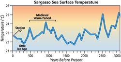
13. I have tested some of Juckes”¬’¢ CVM reconstruction, finding that trivial variations
can yield different medieval-modern relations e.g. Esper CVM without
foxtails; http://www.climateaudit.org/?p=885 ; Moberg CVM using Sargasso
Sea SST instead of Arabian Sea G Bulloides wind speed and Polar
Urals update instead of Yamal – see http://www.climateaudit.org/?p=903 and
http://www.climateaudit.org/?p=887 Juckes”¬’¢ justification for not using Sargasso Sea
SST is not convincing http://www.climateaudit.org/?p=898 , nor is the exclusion of the
Indigirka River series of Moberg et al 2005, which is an extension of the Yakutia series
used in MBH98 – see http://www.climateaudit.org/?p=901
Para 13: The Sargasso Sea series finishes well before the end of our calibration period,
so cannot be used in our reconstruction. It has been used in one peer reviewed
study and cited on at least two web sites with its dating erroneously shifted 50 years
forward, so that the last data point, which represents the 1900 to 1950 mean is instead
presented as the 1950 to 2000 mean. The data file stored at the WDCP is ambiguous
in this respect, but the data was clearly collected at a time when it could not represent
the 1950 to 2000 mean. We have put all the data used in our study online: the Indigirka
series is not available for publication in this way.
The illustration of the Sargasso Sea series by its author (Llloyd Keigwin) in Oceanus http://www.whoi.edu/cms/images/oceanus/2005/4/v39n2-keigwin5n_8723.jpg shows as its last data point the SST from Station S since 1954, which Keigwin plotted together with the reconstruction based on sediment trap information used to calibrate the proxy in the first place (Keigwin, pers. comm.) The figure shown in this image ”¬’ which has been used in several other webpages ”¬’ is not the result of erroneous shifting or misunderstanding of the WDCP archive, but to the inclusion of modern results. In itself, I see no reason why this procedure is more pernicious than the use of tree ring data from both modern living trees and subfossil trees and Juckes has provided no such explanation.
Juckes co-author, Moberg, was required by Nature to supply the Indigirka data, a copy of which I have. If Juckes’ results are unstable to the availability/unavailability of Indigirka results, then the robustness of the results is obviously very questionable.
14. Juckes et al Table 1 contains numerous geographical mislocations. Table 1 shows
lists the Tornetrask site 4 times under different alter egos, using 3 different coordinates,
none of which are correct. The two ”¬Åindependent”¬? foxtail sites are only about
30 km apart (the coordinates being inaccurately reported in Juckes et al.) The Union
reconstruction used two different versions of the Tornetrask site (which are obviously
not ”¬Åindependent”¬?) and neither justified this duplicate use nor the similar duplication of
foxtail and bristlecone sites.
Para 14: The geolocation information does not affect the results: it will be corrected in
the revised version.
Juckes used two different versions of the Tornetrask series, presumably on the basis that they thought that they were from different places. The effect of correct geographic locations will be to show double use of the Tornetrask series ”¬’ which is hardly justified. The Tornetrask site actually extends a considerable distance. The two foxtails sites are closer together than the extremities of the Tornetrask site. Two bristlecone sites from the same gridcell were also used. No justification for using multiple versions of these highly problematic proxies was provided. I note that his reply to Mark Rostron says that the revision uses 13 proxies, so maybe they’ve combined some of these in the revision, although he doesn’t admit this here.
15. Juckes failed to evaluate the validity of individual Union proxies in light of criticisms by
the NRC panel and others. The use of percentage G. Bulloides as a temperature proxy
was criticized by David Black, author of a G Bulloides series from Cariaco. Without
addressing such criticisms, Juckes et al used a percentage G. Bulloides series from
the Arabian Sea in the Union reconstruction – see http://www.climateaudit.org/?p=957.
The NRC panel specifically said that strip-bark bristlecones and foxtails should be
”¬Åavoided”¬? in temperature reconstructions. Without addressing this criticism, out of only
18 proxy series in the Union reconstruction, Juckes et al used no fewer than 4 bristlecone
and foxtail series from one gridcell.
Para 15: There is some confusion here between the requirements of different analytic
approaches. The revised version seeks to make our modelling assumptions clearer. In
particular, we do not assume that the signal to noise ratio in individual proxies is greater
than unity. A simple estimate suggests that is not. In this situation selecting proxies
on the basis of their individual correlations with temperature is inappropriate. The peer
reviewed literature does not have clear evidence of a substantial CO2 fertilization effect.
We note that all the proxies are influenced by factors other than temperature.
I must admit to being puzzled by this response. I asked Jean S about the relevance of assuming that the signal-to-noise ratio is greater than unity and he was stumped. The original article doesn’t mention assuming that the SNR ratio is less than 1.
The issue here is the use of spurious proxies. Juckes et al state: ”¬ÅIt is clear that the proxies are affected by factors other than temperature which are not fully understood. We are carrying out a univariate analysis which, by construction, treats all factors other than the one predicted variable as noise.”¬? But is this assumption a reasonable one? The statistical appendix is based on the assumption that the noise has white noise properties. But if the ”¬Åproxy”¬? is substantially affected by non-climatic factors (e.g. Fertilization), then this model ceases to apply. This is not an incidental concern, as much of the present controversy derives from the use of bristlecone and foxtail pines in temperature reconstructions (both directly and through the weightings of the Mann PC1). The peer reviewed literature has many caveats against the use of bristlecones as a temperature proxy (e.g. Biondi et al 1999), with the explicit statement by that the NRC Panel that these series should be ”¬Åavoided”¬? in temperature reconstructions. CO2 fertilization has been raised as one explanation for the problem with this data, but there are other possibilities (e.g. airborne phosphate or nitrate fertilization). The issue is not whether the particular phenomenon of CO2 fertilization has been proven in the literature, but whether bristlecones and foxtails should be used once again in the face of adverse cautions in prior literature and by the NRC Panel. See also his response to Mark Rostron on bring the proxies up to date.
16. There has been extensive discussion of various aspects of Juckes et al at
http://www.climateaudit.org – see http://www.climateaudit.org/?cat=36.
Para 16: Extensive and ill-informed.


45 Comments
Summary of Juckes reply: “La, la, la, I’m not listening to you”
Steve,
I apologize for not telling you earlier, but its a new feature of WordPress 2.1
If you go to the writing page, and hit [alt]+[shift]+v then a second menu bar appears, and one of the buttons is text colour.
I don’t think Juckes is going to get his Union Reconstruction published and I would not be surprised if he withdraws the paper for some reason rather than have it rejected.
I had hoped that Juckes would be able to substantiate his allegations that there are gross errors committed by you and Ross, but he comes nowhere near justifying the statement. I am concerned that repeating the same unproven assertion over and over appears to be the equivalent of a scientific fact in some circles.
I’ve wondered for the past two years Steve, whether you are a very capable statistician or that some climate scientists are making you look good. Certainly what Juckes et al have produced is wholly derivative, the methods are extremely uninnovative, the statistical control and data quality as diabolical as Mann’s.
Why can’t Juckes go through the recent literature piece by piece and make his case properly? Is he tired? Is it beyond him?
The whole effect is rather like watching Uri Geller do the same five conjuring tricks over and over for the last 30 years and calling it psychic ability well past the point where there’s any credulity left in the audience.
This seems to be rampant in climate science; e.g., “the science is settled.”
I am experiencing a visceral reaction to Jukes’ tone and content. It is a reaction similar to that of enountering a type of psychopathic tendency within a person who is doing something sinister or dishonest.
In my mind Jukes has totally discredited himself. If this paper is published it will be a travesty. If I was one of his coauthors I’d be running from this thing as fast as possible.
While this question might suggest that I am stupid, it would seem to me that surely you need a S/N ratio greater than one, otherwise how can you be confident that you have and can extract a signal?
Can you assume that the noise has certain properties such that you can cancel it out?
#3
Wasn’t Geller going gang-busters until he appeared on the Tonight Show with Johnny Carson? It seems that Carson had started his career as a professional magician and was aware of all the slight-of-hand tricks one could try to pull. Geller claimed that he was too nervous to perform that night, but it seems the world figured out that a good magician could see things that serious journalists and even some scientists at the time were bamboozled by.
I had the pleasure of meeting James Randi around that time (1974 if I recall correctly). After he did his act he invited anyone who was interested to stay after for a lecture on the paranormal. Uri Geller was one of the subjects of his discussion. According to Randi, Carson called him for advice on how to handle Geller. The result is history. Randi also did the spoon bending trick, with my car key, and then showed us how it was done.
re #3 & #6
Come on. You know the paper is going to get published. Along the lines of “you can get a grand jury to indict a ham sandwich”, you can get a journal to publish a ham sandwich, as long as the ham sandwich points to AGW. I am sure Dr. Juckes is reading Steve M’s and Willis’ comments, and he will get a big smile on his face if/when his paper gets published. However, over the long term, this great heyday of AGW paper publishing is going to be reviewed and the authors are going to regret the overselling of AGW.
10: Nope, there’s too much publicity, and even THAT journal does not want to go down in flames. I’ll bet that the journals are wising up, since the editors know thaey are on thin ice. Credit Steve, Warwick, Willis, Pielke, et. al. for getting this science back on track. It’s over for the “consensus” boys, IMO. There are too many brilliant scientists and lay eoople out there, and the Internet has made a HUGE difference. Even the media realize this. I have HOPE!
If I remember correctly, Geller repeatedly sued Randi after Randi correctly called him a fraud. Geller still made life difficult for Randi. Does anyone know more of this story? Just because someone is blatantly right and someone is obviously wrong, it doesn’t mean that truth automatically wins. You still have to fight even if you are right. Steve will still have to fight hard even if the equations show that he’s right.
The Juckes et al paper has turned into a very interesting demonstration of the professional standards considered appropriate by climate ‘scientists’.
It is interesting, and indeed surprising, that the co-authors of the paper are willing to associate themselves with this chain of events. In addition to M N Juckes, co-authors listed are M R Allen, K R Briffa, J Esper, G C Hegerl, A Moberg, T J Osborn, S L Weber, and E Zorita. One wonders whether they have each given their assent to M N Juckes to represent their views. One must assume that as they are listed as co-authors, that they have indeed given their assent, and so choose to stand beside M N Juckes in this discussion.
In other fields, individuals being seen to act the way Juckes et al are acting would likely be held accountable by the professional associations of which they are members. Are climate ‘scientists’ members of a professional association that is committed to maintaining high professional standards? If so, I would expect that they may soon hear from the appropriate person in that organisation.
If climate ‘scientists’ are not required to be members of a professional organisation, that in itself speaks volumes.
Over at http://www.climatesci.colorado.edu, Roger Pielke Sr is hosting threads by Hendrik Tennekes entitled Unlicensed Engineers that are addressing related climate science issues, although more focussed on the modelling aspects. In his opening remarks, Hendrik Tennekes says:
The engineering analogy seems appropriate to me. One of my beefs about the NAS report was that they concluded that bristlecones (strip bark) should be “avoided” in temperature reconstructions. Compare that to an engineer saying that Grade-D concrete should not be used in bridges. They then presented several alternative reconstructions all of which used bristlecones, without investigating whether theuy used bristlecones. Can you imagine someone with an engineering license doing this? It’s inconceivable. And yet this was a blue-chip academic panel (and not the worst one by any means).
re #7
Why would that be? In GPS (UC/Mark T, please correct me if I’m wrong), for instance, SNR is well below the noise level (typically -20 to -30 dB I’ve been told), and still you can extract the signal. Furthermore, Juckes’ wierd statement appears also in his reply to Mark’s comment about local correlations. If the noise is uncorrelated with the temperature (as it should), then theoretically the proxy SNR does not matter at all. With all the best of my understanding, I just can not figure out the meaning of this Juckes’ statement. Maybe I’m the one who’s stupid.
OT: I doubt Geller ever laid a legal glove on Randi. I saw Randi in Sydney many years ago, and his spoon bending was sublime.
#15
yep,
S is well below the noise level
http://en.wikipedia.org/wiki/High_Sensitivity_GPS
see also http://www.climateaudit.org/?p=1230#comment-93048
Pardon me, I’m just an amateur, but isn’t the fact that the GPS signal’s properties (shape & frequency) are known in advance the reason why it can be found despite a low SNR? I figure it’s also important that it’s highly regular/repetitive.
If, on the other hand, you’re trying to determine what the signal looks like – rather than just find a known signal within the noise – then surely you either must understand the properties of the noise very well so that you can cancel some of it, or else have a high enough SNR that the signal is apparent. Otherwise, how can you tell whether the “signal” you found is really a signal, or just an artifact of the noise? Or possibly some of each? Additionally, what if there are multiple signals – like what you’d get from say two competing GPS networks with similar signal properties – how do you tell which one is which?
I don’t think you can easily compare the two situations.
#18: Nicholas, you are right, but the situation in this case is very similar: the signal properties are known (the instrumental record). Beyond that, there are other ways of “extracting” the temperature signal even without the knowledge of the instrumental record assuming the linear proxy model holds, see, e.g., here. The fact is that the Team is using ancient techniques with could be easily improved, but there is no point of doing that if you really do not believe in the current proxy model.
I would think that if you had a long enough time series of your signal, and then used Fourier to convert it from the time domain
to the frequency domain, that as long as the signal you were looking for was regular and repeated, it would stand out from the noise.
As the randomness of the noise would cause it’s frequency to spread out more or less evenly.
At least that’s my recollection from 20+ year old math classes.
#20: Mark, you would be an ideal student, remembering the main idea after 20 years… wish we had more of those nowadays! The fundamental idea of separating noise from the signal is to have something which makes the distinction between those two. It can be the frequency domain representation or some statistical properties, whatever. It all depends what you assume from your system. SNR below “unity” only tells that the variance of noise dominates that of the signal, nothing more. There might be other properties which allow the seperation, e.g., noise is Gaussian while the signal is not or you may have several measurements (e.g., many proxies from the same area). Time, frequency, or some other domain characteristics may be different, and so on.
Re: 21
Jean, might one analogy be the clear extraction of a weak, carrier-based FM (frequency modulated) signal from among AM (amplitude modulated) noise strong at the same carrier frequency?
Re #22
It might, except that the tree rings contain AM signals only
Actually, I’m currently working a problem where the inherent SNR is around -35 dB at best, and as low as -55 dB worst case. PCS cell phones operate with a nominal SNR of about -9 dB, but they have known codes and waveforms and integration brings the symbol to noise ratio (Es/N0) to +7 dB or greater. Per Nicholas’ comment, yes, knowing the structure of the underlying signal is beneficial, and sometimes necessary, particularly in an extremely high noise environment such as what I’m implementing. However, it is not _always_ needed. For example, if your signal has a much lower bandwidth than the original data set, you can filter and decimate to reduce the noise power level. Every power of 2 decimation is 3 dB “gain” over the original SNR in such cases (one must be careful not to decimate past the critical sampling rate of the original signal, however).
Obviously with any method, the higher the noise the less likely you are to find the original sources. There is no magic “line in the sand” however, that requires above unity (0 dB) SNR. Adjusting the value either way simply changes a) the probability of detection or b) the amount of required processing to achieve the desired probability of detection.
FFT methods are no different than any other. Should the noise be too high, you cannot discern the “peak” in the result from spurious peaks due to noise alone. Since an FFT is nothing more than a point-by-point integration modulated by a complex exponential, you are essentially correlating and integrating the signal, providing the same type of gain as a filter and decimate function. The same goes for wavelet decompositions (Moberg’s “magic” bullet).
Mark
re: #19
The problem is, of course, that to all intents and purposes the signal is nothing but a rising trend. Therefore finding the “signal” among noise is simply a matter of finding proxies with a rising trend in the instrumental period. And this is what, of course, MBH98 did in an automated way by its off-centered “PCs”. But once suitable proxies were identified, this method isn’t needed, one can simply select the ones which are wanted and hang on to them for dear life. Who cares what mere NAS panels or statisticians say. As long as you can get away with saying, “The idea that data can only be used once is going to need a little more justification before it gains wide acceptance”, you’re home free.
It should be mentioned as well that the signal properties are only “known” for the duration of the instrumental record (and even then there is a fairly large error in the signal). Stating that these properties hold for any period (future or past) outside of the instrumental record is disingenuous. The trend of a sine wave near zero looks like a line, but that hardly describes the sine wave itself outside of that region.
Mark
Hmmm, did you mean to say that the trend of a sine wave near zero looks like a straight line …?
Yes, straight line was my intended meaning.
Mark
Looks like my comment got whacked. Where’s Lee when I need some “censored” companionship? 🙂
Yes, straight line was my intended meaning. Generally, I refer to non-straight lines as curves, though that leaves ambiguity for the rest of you attempting to decipher my “Mark-speak.”
Mark
Mark, you’ve got to get used to waiting at least a half hour before worrying about a message not appearing. Seem my complaint on the How is Climate Audit Set Up thread. Apparently there’s no practical solution just now.
Yeah… I thought it got whacked because it actually appeared on the sidebar for a moment, then disappeared.
Mark
I have some direct knowledge of “high sensitivity GPS”; friends produced the first version of that technology, which is now embedded in many cell phones (google GPSone).
I think there’s a simple and very important distinction between extracting GPS and climate signals: the nature of the noise.
The GPS signal, as noted above, is at a known set of frequencies and periodicities. The noise in which it is embedded is very different from the signal. IIRC, the noise is generally quite random, nicely averaging out to nothingness over many samples. I could check to see if sample charts are available.
On the contrary, the climate signals discussed are incredibly similar to the “noise”. Most proxies for temperature (even “real” thermometers!) are susceptible to incorporation of “noise” from many possible sources such as precipitation, pressure, seasonality, insolation, wind, forest succession cycles, urbanization and so forth. The interesting thing about ALL of these “noise” sources is how alike they are to the signal being sought.
Measuring temperature accurately, under controlled conditions, is quite difficult. (When’s the last time you tried getting a thermometer to read 0.0C/32.0F in an ice bath?) It continues to amaze me that scientists so blithely presume they can extract useful temperature information from a hodgepodge of data. Just because a computer is involved doesn’t make the results any better. Some might even claim GIGO. 🙂
Re: #32
Some years ago I was responsible for thermometer calibration where I worked. I actually used a water triple point cell, an NIST (they may have still been NBS at the time) calibrated standard platinum resistance thermometer and a high precision resistance bridge. I do have some idea how difficult it is to accurately measure temperature with millidegree precision and it never ceases to amaze me how otherwise intelligent people think it’s possible to accurately and precisely extract a few millidegrees/year signal from a very noisy record even in the absence of significant systematic error, especially when there is no real standard reference method for comparison.
And in this case, the unwanted noise (precipitation, for example) often looks exactly like sought-after signal. In fact, other researchers would say many of the measuring devices in use are designed to measure “noise” (e.g. precipitation), and any other components seen are truly noise.
What a sorry mess. (Written as the first rain of the year comes down… and also the first above-freezing night of the season approaches. Wait! Perhaps precipitation is a proxy for temperature??!! And the snow outside is melting. So clearly, increased rainfal causes localized warming here… :))
Guys, I think your assumptions are a little incorrect here. IF a signal does exist, then it IS possible to extract said signal with enough processing. More proxies, more filtering, more signal processing in general, will allow extraction. The reason is that IF there is a signal, then it will have non-Gaussian properties, and a sufficient amount of properties will allow some processing method to distinguish the signal from the noise.
Of course, in the case of tree rings, the _hypothesis_ is that temperature is the primary forcer and all other sources of tree-ring growth are either a) noise-like or b) insignificant enough to ignore. While the temperature does resemble noise, the case goes, there is an underlying trend in the noise towards rising temperatures. Unfortunately, nobody has ever been able to show where the hypothesis of temperature=tree-ring width has been tested, and in fact, the most comprehensive test ever done was recently released and stated something quite different: moisture is the primary driver of tree-ring width, particularly for the bristlecones. Ooops. Note that Steve Sadlov has _repeatedly_ made this claim, on deaf ears to all but those of us in here.
Oh, and for the record, the GPS signal actually very much resembles the noise in which it is embedded. GPS is direct sequence spread spectrum (DSSS), which is designed to be look like Gaussian noise over a given bandwidth. Within that bandwidth, noise and signal are indistinguishable except for the fact that there is a known pseudo-random sequence with which a demodulator can decorrelate (despread) the signal back to its original structure (information bits). The same (or very similar) method is used for standard PCS cell phones in the US, though each individual user is spread with his own code, each code designed to have very low cross-correlations with shifted versions of itself and other users’ codes.
Mark
Mark, it depends on how you are thinking of the “signal”. It seems to me, you are suggesting the “signal” is the “growth rate” or some such of the tree. However, people who are using proxies in multi-proxy studies are treating the proxies as if there is a “temperature” signal in there somewhere (presumably along with a precipitation signal, a CO2 signal, a fertilizer signal, an insect strike signal, etc. etc.).
So my point is, given that they are trying to extract one of what is surely many signals in the proxy, how do they know they got the right one? Even worse, if they are making assumptions about the shape of the signal (e.g. that it’s a rising trend), then the proxies can no longer tell them whether temperature is rising or not – they’ve already assumed that as part of their signal search.
So, your point confirms mine. The GPS signal has *known* properties. Not guessed, not assumed, known. The “temperature” signal, from a proper neutral point of scientific interest, has no known properties. It’s those very properties that we’re trying to *determine* from the proxy. Going in there with a predetermined idea of what the signal is that we’re trying to extract, is not going to help us discover the properties of the signal. Now, there ARE some things we know about the temperature signal that we can use – such as its autocorrelation parameters, standard deviation, etc. – from what I can gather, those things tend to be fairly similar in temperature series. But the trend itself is what we’re trying to determine so we can’t start with any assumption about that.
So, to sum up, you can think of there being one signal, or many signals. If you think of there being one signal, then successfully extracting it does not necessarily give you temperature, as temperature is only one component of the total signal. If you think of there being multiple signals, how do you know which one you are extracting? And again, it comes back to the point that with GPS etc. despite the fact it may look like noise, we still know a lot about its properties, so that we can distinguish it from noise. We know far less about temperature signals – especially if we’re not going to even bother correlating the proxy to local temperature records.
Mark, There is a limit to what you can accomplish with signal processing because any processing introduces new errors. At some point, it is not possible to recover even a known signal from the noise. I think this is basic conclusion of information theory.
Actually, the growth rate is the “observation.” The “signal” would be temperature.
Mark
There is always error associated with signal processing. Information theory simply puts a bound on the amount of information vs. amount of noise (ala Nyquist, for example). In the context we’re discussing, the “signals” are very slowly changing compared to the inherent noise, i.e. they have a much narrower bandwdith. Each additional observation (proxies), coupled with filtering (and decimation) serves to decrease the noise bandwidth to that of the signal, making detection more probable (note that there is always a probability of a false detection, as well as a probability of no detection).
The problem with the tree-rings, however, is not necessarily one of noise. It is actually one of attribution: nobody has ever definitively determined what each signal actually represents. PCA, ICA, MCA, regEM, etc., do not identify signals… a-priori knowledge must exist to assign the results to known signals. Said knowledge does not exist. In fact, recent studies (the only I’ve ever heard of) seem to indicate that temperature is not even one of the signals (in the case of the BCPs).
Mark
This point cannot be emphasized strongly enough. However, the signal to noise problem I was referring to was extracting the long term temperature change from the instrumental temperature record. While in theory it should be possible to correct the readings at each station for systematic errors, remove the high frequency noise by low pass filtering and increase the precision from +/- 0.5 degrees to a few millidegrees by averaging over a large number of stations, in practice it is not possible to achieve the necessary precision because the information to correct all the errors just isn’t available.
It’s also a point that folks like Schmidt and Mann seem to gloss over. Oddly, the tree-ring/temperature “linear relationship” is mentioned in MBH98, with a notation that “absent such a relationship, these results are meaningless” (paraphrased), yet nobody seems to care.
It’s not even +/- 0.5. According to GISS, it’s +/- 1. I think the problem is not one of “information just isn’t available,” it’s one of “we don’t know how much is available.” This a direct result of the unwillingness of interested parties to release their coveted data and methods.
Mark
RE: #33 – Meaurement Systems Analysis 101 …. a course that the Hockey Team either hated, slept through or flunked …..
#41
Ah, those at least three fundamental assumptions .. 🙂
But you need to be careful, MBH98:
Maybe one or more are exclusive, IOW maybe the model assumes there is a linear dependence in the composite, not in the individual proxies.
RE: #41 – The Team are nervous and defensive. They probably never anticipated having so many “maths of variation” savvy scientists and engineers reviewing their work. Now the steer’s out the gate and they are scrambling to round it up. They are between a rock and a hard place. Expect further intesification of obfuscation.
You have a great blog here and it is Nice to read some well written posts that have some relevancy…keep up the good work 😉