One of the reasons why scientists have been so quick to use tree ring information despite all the problems is that, for the most part, there is excellent dating control on tree ring chronologies, something which can be problematic in other proxies.
Today I want to document some notes on dating the Arabian Sea G Bulloides. In this case, although Moberg (and Juckes) present one series in their data sets, this series actually results from a splice of information from two different cores – a splice not actually made by the original authors (although one of their figures is suggestive), but by Moberg. But how legitimate is it to splice the two cores?
Today I’ll look at some potential problems with homogeneity of the splice and also with even dating the cores.
Here once again is the figure from Anderson et al 2002 comparing the G Bulloides series to the Hockey Stick – thereby placing this data squarely on Team radar (and thus Moberg used it in his influential reconstruction even though there was no direct relationship of the proxy to local temperature – actually the opposite: the proxy was inversely related to local SST.
Another thing to observe here: note that the original authors do not use the percentage G Bulloides directly, but instead use the square root of the difference in composite G. bulloides abundance with respect to the 1975 average (thick line). This reduces the very great non-normality of the G Bulloides percentage data – a precaution abandoned by the Team.
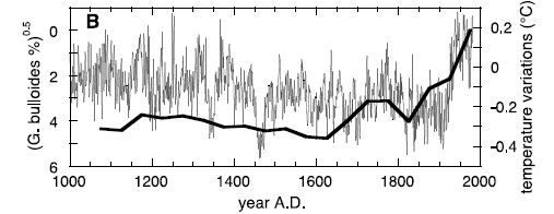
Anderson, Overpeck et al 2002. Fig. 2. (B) Time series of Northern Hemisphere temperature variations from (28 – MBH) (thin line) superimposed on the index linearly related to monsoon wind speed, the square root of the difference in composite G. bulloides abundance with respect to the 1975 average (thick line).
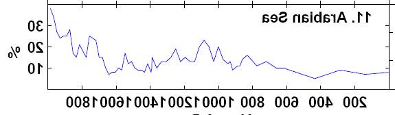
Now here’s a figure of Moberg’s version of this proxy. A couple of important differences: the proxy goes longer than in the Anderson et al 2002 article (this is not a problem in itself as Moberg refers to a later version in Gupta et al 2003); perhaps more important is the abandonment of even a token attempt to normalize the data. Moberg’s SI described the splicing as follows:
A combination of two marine sediment records from the Arabian Sea14-15 in which the percentage of the foraminifera Globigerina bulloides reflects the extent of ocean up-welling, which is determined by the strength of monsoons, which in turn indirectly reflect both summer and winter large-scale temperature changes through the differential seasonal heating and cooling of the Asian continent and surrounding oceans16. We used data from Core 723A15 for the early years up to 1390 A.D. and data from Core RC273014 from 1391 to 1986 A.D. (c.f. Fig. 3c in ref. 15). Although this record reflects temperatures only indirectly, it was included to improve the balance in the geographical distribution of proxy sites.
This latter point seems somewhat of a bait-and-switch to me and rather misleading: actually it’s untrue that the “record reflects temperatures only indirectly”. The proxy actually records temperature rather directly – the negative correlation between percentage G Bulloides and water temperature is actually rather strong relative to other proxies in the network.
The only thing that’s “indirect” is that colder water offshore Oman is held, I guess, to be indirect evidence of global warming, while of course warmer water offshore Oman in the CRU data is held to be direct evidence of global warming. I guess this makes sense to real climate scientists.

Moberg et al 2005 Version of the Arabian Sea G Bulloides series
Next here is Gupta et al 2003 Figure 3 which illustrates G Bulloides values from two different cores: RC2730 and 723A. An overlap between the two cores is shown from about 900-500BP. A horizontal flip of the Moberg version is shown to evidence that these are the same plots.

Gupta et al 2003. Figure 3. G. bulloides percentage in Hole 723A (filled circles) and box core RC2730 (open circles), showing also dated depths in 723A (plus signs) and RC2730 (crosses). The North Atlantic Medieval Warm Period (MWP) and Little Ice Age (LIA) extents are based on the records shown here.
There are a few interesting points to this graphic:
1) the most modern values shown here are under 30% G Bulloides, while the most recent values in the Moberg version are over 30%. The Moberg version is consistent with RC2730 data archived at WDCP, – my graph of WDCP data here – but the published illustration omits the two latest values in the archive – both of which are high. Why is that?
2) the general tenor of G Bulloides percentages in this Figure prior to the most recent values are under 15% and most are under 10%. These low values are associated with water of at least 26 deg C i.e. no upwelling. As noted in my previous post, high G Bulloides percentages are associated with water of about 22 deg C. Taken at face value, these G Bulloides values indicate very low monsoon strength prior to the modern period.
These core values seem to prove too much – the monsoon strengths indicated here seem too weak and I thought it would be a good idea to take a look at the splicing and the dating. Here are age-depth plots for RC2730 and 723A on the same scale with radiocarbon points marked with solid circles. Points at which there are G Bulloides measurements are marked with red + (RC2730) and o (723A).
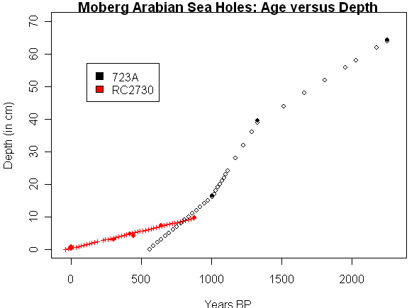
Age-Depth Plot of Cores RC2730 and 723A with radiocarbon points.
Again a couple of quick observations:
1) the implied deposition rate of 723A (31 cm/ kyr) is over three times more rapid than the implied deposition rate of RC2730 (10 cm/kyr). This seems to me to be a big inhomogeneity: could this be related to G Bulloides levels? I don’t know, but it seems odd to splice two series of percentage G Bulloides from cores with such different deposition rates. (Update: Richard T observes below that the different deposition rates could result from different coring methods, with one core mixing more mud with the core. I don’t know how likely this explanation is, or whether it’s merely an idea.)
2) Only part of RC2730 has been reported. Anderson et al 2002 report that the core was 51 cm long, while only the top 10 cm has been reported. It would be interested to see whether the proposed correlation holds up over the rest of the core. I’m not suggesting that it won’t – it just seems odd that the job would have been left half-done.
3) Notice that the radiocarbon points for the two cores do not overlap. The oldest radiocarbon measurement for RC2730 is younger than 723A. (BTW there appears to be an older portion of RC2730, but no analysis has ever been reported.) The top part of 723A is said to be about 500BP but this is not based on any measurement, but, as far as I can tell, on nothing more than extrapolation and/or wiggle matching. I wonder why they wouldn’t have tried to date the core top. If the failure to report a top date for 723A seems surprising, here’s what they said in the Nature SI:
To determine the age of the uppermost sample, we correlated the top of our record with a well-dated Oman margin box core (RC2730), finding an age of ~560 yr, suggesting that the top few centimetres were lost at the time of drilling.
and again:
Fig. 1s. Hole 723A calendar age versus depth. Ages were corrected using the Calib program HTML version 4.2 (http://depts.washington.edu/qil/calib/) and a reservoir correction (delta R) of 207 years. The one-sigma uncertainty is shown by error bars. The core top age (circle) was estimated by stratigraphic correlation with well-dated box core RC2730, and one depth (2.18m) was not used in the age model.
I’m not sure what “stratigraphic correlation” means in operational terms in this case. I don’t think that it means “stratigraphic correlation” as practised by geologists, but merely the wiggle matching of Gupta et al 2003 whon above.
Radiocarbon procedures for core RC2730 were explained in Anderson et al 2002 SI as follows:
We sampled two Soutar box subcores at continuous 2-mm spacing using the method developed for Cariaco Basin sediments (22) (supporting online text). Nine AMS (accelerator mass spectrometry) 14C dates on planktonic foraminifers from core RC2730 provided the age control (fig. S1). When corrected for the average reservoir age of the Arabian Sea (23, 24), the uppermost four samples, including the replicated 0- to 2-mm sample, were too young (less than zero age), which can be explained by the presence of bomb radiocarbon that has mixed downward over the upper 10 mm (table S1). Each of the box core sediment surfaces was observed to be pristine during core recovery. This observation, combined with the presence of bomb radiocarbon in the upper samples, supports our assumption that the top of the box core corresponds to the date of collection (1986). We constructed an age model by fitting a line through 1986 at the core top and through the remaining reservoir-corrected, nonzero 14C dates [the corrected age at zero depth (black symbol) in fig. S1 is the inferred age of “36 years (with respect to 1950)]. The date for 40 mm is too old to fit the linear sedimentation rate model, and we discounted this date because it comes from the minimum in G. bulloides abundance, where mixing could most easily bias the age. All the 14C dates were determined on the core with the highest sedimentation rate (RC2730),
The reservoir age was not reported here, but I’ve seen a figure of 604 years elsewhere:
An average reservoir age of 604 years was calculated for the western Arabian Sea, based on 14C measurements of known age mollusc, gastropod and coral samples from 7 sites in the region (Southon et al., 2002). However, a detailed study determined that the reservoir age of the Northern Arabian Sea has varied from 600-1200 years during the Holocene (Staubwasser et al., 2002). This large range in “possible” reservoir results in adding significant uncertainty to any Arabian Sea chronology.
I’ve also been keeping my eye out for any other information on G Bulloides percentages in the Arabian Sea (as I’ve reported eslewhere, percentage G Bulloides at Cariaco, Venezuela is used as a wind speed proxy by Black et al – who condemned its use by Soon and Baliunas as MWP evidence.
(On a previous occasion, David Black showed up briefly here, but when challenged to be consistent i.e. either condemn Moberg’s use of G Bulloides as a temperature proxy or withdraw his criticism of Soon and Baliunas, David Black quickly, and all too typically, disappeared.)
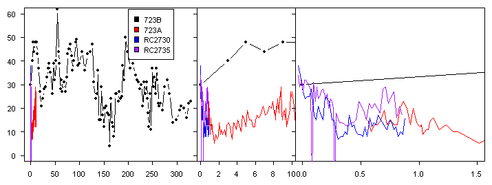
Anyway here’s a graphic showing G Bulloides percentages for 723B, RC2735 as well as 723A and RC2730 on three different scales: left long (300,000 years; middle -the Holocene 10,000 years; right – recent 1500 years.) 723B was sampled at coarse intervals, but even this coarse sampling indicates that G Bulloides percentages above 30% (as in Moberg) are far from unusual on a long-term basis. Do the high G Bulloides values in ice age periods indicate high monsoon levels or simply cold water. A question for another day.
References:
Anil K. Gupta, David M. Anderson & Jonathan T. Overpeck, 2003. Abrupt changes in the Asian southwest monsoon during the
Holocene and their links to the North Atlantic Ocean, Nature.
David M. Anderson, Jonathan T. Overpeck, Anil K. Gupta, 2002. Increase in the Asian Southwest Monsoon During the
Past Four Centuries, Science.


19 Comments
In the UK, we used to have a wonderful comedy act, called Morecambe and Wise. Morecambe, who was bald, used to rib Wise’s full head of hair by implying it was a toupée, by lifting his fringe and saying “You can’t see the join!”
That’s how I react when I see these splices of clearly disparate data into a single narrative which is meant to imply something anomalous about modern climate – “You can’t see the join!”. It would be tragic if it wasn’t so comic.
The lack of the two most recent datum points in Gupta’s figure is probably so the graph can stop at 0 yr BP (i.e. 1950), rather than continuing to -36 yr BP (1986). This simple expediency makes the graphs neater, and does not affect Gupta’s interpretation.
Perhaps this from Anderson et al. 2002 would help explain the core correlation: “second core was stratigraphically correlated to the dated core by a combination of the G. bulloides, calcium carbonate, and coarse fraction stratigraphies.”
The very different sedimentation rates between cores is probably an artefact of the coring device used. Remember these are soft muds, not solid rock, and can be deformed in coring. Some corers tend to suck in additional material, and expand the sequence, others push mud out of the way and reduce it.
There is a database of marine reservoir corrections by Reimer available from http://www.calib.org
To determine if the glacial abundance of bulloides was monsoon generated or simply colder SSTs we need to look at other proxies. For example, the difference in d18O between bulloides and ruber from the same levels is a measure (in this location) of seasonality.
It really would be most helpful if you gave the references for the papers you cite.
Steve, it would help the visual readability of the article, to briefly highlight the chronology L<->R “flip”. A good place might be between the Moberg 2005 and Gupta 2003 graphs. Inserting a reversed Moberg 2005 would be pretty simple, and emphasize the shift (for the rest of the article) from datas to Years BP.
I’ve added refs to Gupta and Anderson and shown a flip of the Moberg image. Richard, as to the different sedimentation rat4es, you state:
Jeez, this is even more worrying. Their datum here is percentage G Bulloides. If it is an issue of whether extra materials were being sucked in by one corer relative to another, then this is going to affect percentage G Bulloides and mean that a splice of this statistic from different cores could be quite perilous. It wasn’t an issue that I had in mind but since you raise it, why wouldn’t this mean that the splice is fraught with a big potential homogeneity problem?
BTW you say that the following phrase should help but I didn’t find that this explains very much.
Geez, and I thought tree ring studies were stretching the limits of credibility! It is much worse, if the Team is selecting proxies that are NEGATIVELY correlated to their choice variable and presenting them as POSITIVELY correlated. Do I have this right?
#5. If one looks at the most detailed information, percentage G Bulloides is negatively correlated to SST offshore Oman. This isn’t just a statistical relationship, but has compelling physical support, as there is a great deal known about the respective temperature ranges of G Bulloides versus G Ruber. On the other hand, the gridcell SST shows a temperature increase in the offshore Oman gridcell – creating a conundrum that is not addressed by the Team.
If the SST offshore Oman has been increasing in the 20th century, then the percentage G Bulloides in the core corresponding to the 20th century should be going down. So there’s an apparent inconsistency between the proxy record and the SST record.
The Team theory is presumably that SST offshore Oman is negatively correlated to world temperature. Although this sounds absurd, it’s not as crazy as it sounds. The total surface area of the ocean where you have substantial upwelling is not all that large. Offshore Oman is fairly unusual that way. (BTW you also have upwelling offshore California). There is convincing evidence of high upwelling offshore Oman during the Holocene Optimum and one can envisage atmospheric circulation in which Asian monsoon and extratropical Asian temperatures are associated. So the possibility of a relationship isn’t crazy – however, at best, this becomes a very indirect proxy for extratropical NH temperature – and surely the direct proxies should be preferred. And because this proxy is low-latitude, it gives the impression that tropical temperatures are increasing, while no such conclusion can be drawn from this proxy.
Hmm, more teleconnections.
Steve M, is the sample location close to the shoreline or far from the shoreline? I believe that makes a difference as to the type of upwelling and its connection to windspeed and monsoon strength.
Link
I presume that Anderson and PRell in the link are referring to site 723 – see ftp://ftp.ncdc.noaa.gov/pub/data/paleo/paleocean/by_contributor/anderson1993/readme_anderson1993.txt . This is the locus of the 723A core discussed here and is in the heart of the upwelling zone. The RC2730 core looks to be about 11-12 miles north but presumably still well within the upwelling zone. I suppose that there could be diverging temperature trends in the onshore and upwelling zone SSTs, with the 723 core providing direct evidence only on the relatively small upwelling zone and elsewhere only through teleconnection and correlation.
#4
Flux calculations would be problematic if there are coring artefacts in sedimentation rates. Percentages are robust, provided sediment is being incorporated laterally, which is most probable. Incorporation of sediment from other depths would be no worse than bioturbation, and would tend to smooth the record.
#8
From the supplementary material RC2735 (18° 14N, 57° 36E, water depth 498 m, core length 42 cm), RC2730 (18°13N, 57°41 E, water depth 698 m, core length 51 cm). Gupta’s core is at 18°03.0790N, 57°36.5610E. Google Earth puts these sites about 70km offshore.
#10. I see your point. How probable is that the difference in coring method accounts for the difference in sedimentation rate? It’s too bad that they didn’t report on the rest of core RC2730 or do radiocarbon on the upper portion of 723A.
#2. Richard T, I’d be interested in your thoughts on the situation with coarse described below.
First, Anderson et al. 2002 discusses the connection between cores RC2735 and RC2730 – not 723A. Here is a plot from the archive for Andeson et al 2002 which is related to the statement:
In the absence of any details on how the correlation was effected, I can’t see that the proposed correlation is conclusive. The MWP match between RC2735 and RC2730 doesn’t look very convincing to me.
Another point that I hadn’t noticed before: look at the tremendous increase in coarse percentage in the top 1 cm of RC2730. Is there any climatological reason to expect such a dramatic change in coarse percentage? Or could it be an artefact in which coarser fractions are washed leaving the fines. Here’s the top of the core:
depth_cm bp coarse carb bull
1 0.1 -36 27.1 NA 38
2 0.3 -17 23.9 55.6 34
3 0.5 2 20.6 54.6 27
4 0.7 21 16.0 52.8 24
5 0.9 40 17.0 53.1 25
6 1.1 59 13.5 52.6 25
7 1.3 78 10.0 50.1 28
8 1.5 97 8.8 48.3 17
9 1.7 116 8.4 49.1 15
There’s a strong association between pct G Bulloides and pct coarse, so if there is any artefact in the pct coarse, there will be a knock-on effect for pct G Bulloides. Maybe, by the time that the top 1.5 cm settles into core mode, it will be a lot lower.
Also note that there is no matching coarse and carbonate information for 723A. It’s possible that it was done and then not archived. But it also might not have been done. In any event, they don’t say that they matched 723A through use of all 3 variables and in the absence of a direct statement, I don’t think that you can assume that this is what they did for 723A.
A secondary point: note that using RC2730 without RC2735 enhances the modern-medieval differential.
Steve M, you say:
This is likely because Anderson’s archived data don’t match the description in Anderson’s Science paper. The Science paper says:
The archived data, on the other hand, correlates 34 mm and 93 mm in RC2730 with 50 mm and 100 mm in RC2735. The correlation in the Science paper provides a much better fit, at least visually, to the MWP period.
w.
Willis, what do you think about the changing proportion of coarse fraction here?
There’s a few puzzles about the coarse fraction here. The data looks like this:
The two records move about in parallel from ~1150 to ~1300. From there, in Hole RC2735, the coarse fraction is steadily decreasing for about 400 years, up to ~ 1700. In RC2730, on the other hand, it is steadily increasing for about 500 years, to about 1800. From there, both of them increase rapidly to the present.
Part of the reason may lie in the undersea geography of the region:
As you can see, RC2735 is at an escarpment the edge of an upper plateau, which falls down to a lower plateau where RC2730 is located. Because of this, the coarse fraction will be very sensitive to the exact direction and depth of the currents in the area. If the current is running across the escarpment, there will be a large speed difference over the two areas, which will change the coarse fraction.
Alternatively, the presence of the escarpment may mean that the deeper plateau is swept by an entirely different current than the upper plateau.
Next, the coarse fraction is related to the dissolution rate of the shells. There’s a discussion of this in the paper Coarse fraction fluctuations in pelagic carbonate sediments from the tropical Indian Ocean: A 1500-kyr record of carbonate dissolution. In that paper, they say the changes in coarse fraction:
However, if monsoon strength were the only reason, we’d expect the two records to move in parallel since the winds will be quite similar at two oceanic sites that are only 10 km apart … but they don’t move in parallel.
Finally, the fact that the increase is all in the top couple of centimetres at least allows for the possibility that the fines have been partially washed out of the top of the sampled core.
w.
An oddity about the Anderson paper in question. The abstract says:
That seems like a quite clear conclusion, monsoon winds are on the rise, and pretty sharply if their figure is any indication. Figure 2 of the Anderson paper (see original post above) says that monsoon wind speeds have increased fourfold from 1840 to 1975, and by 2-1/2 times since 1890!
But then they go on to say:
Translation: instrumental records show no change in the last century in monsoon wind strength, drought events, or rainfall, but by gosh, that doesn’t mean that our conclusions are wrong.
Say what?
w.
Re: #16
Write a letter to the Editor and ask if there was any editorializing of the wording of the abstract. It is standard policy with Nature and Science to take some editorial liberties at this level. And this sometimes leads to Abstract-Results rhetorical disharmony.
I thought the normal practice with proxy data is:
1. plot the proxy data
2. plot the appropriate instrumental data (temperature, windspeed, etc)
3. demonstrate, over an appropriate period, that the proxy data correlates with the instrumental data
In this case they can find no instrumental data that correlates with the proxy data, but they proceed with their paper anyway? I wonder if the Mann hockey stick was their “instrumental” record.
Regarding coastal upwelling, it’s a function of both windspeed and wind direction. Changes in upwelling at a location may reflect shifts in mean wind direction as well as changes in windspeed.
#11
I’ve worked on age-depth models on cores from the Norwegian Sea where the difference in apparent sedimentation rate between the box-corer collecting the surface sediments and a piston corer collecting the Holocene sequence is this large. How much the piston corer stretches the sediment will depend on the sediment properties and on how details of how the particular corer is deployed. In this case, the two cores are some distance apart, so differences in bed topography focusing sediment may also be important.