In a recent post, I noted the discrepancy between the UK Met OFfice contribution to IPCC AR5 and observations (as many others have observed), a discrepancy that is also evident in the “initialized” decadal forecast using the most recent model (HadGEM3). I thought that it would be interesting to examine the HadGEM2 hindcast to see if there are other periods in which there might have been similar discrepancies. (Reader Kenneth Fritsch has mentioned that he’s been doing similar exercises.)
In the figure below, I’ve compared HadCRUT4 (anomaly basis 1961-1990) to the Met Office CMIP5 contribution (red), converted to 1961-90 anomaly.

Figure 1. IPCC CMIP5 contribution (HadGEM2 RPC45 average) vs HadCRUT4.
There is a persistent over-estimate over the first half of the 20th century, particularly in the 1920s. Nor does the Met Office model adequately replicate the temperature increase of the early part of the 20th century. In its CMIP contribution, the average temperature in the first decade (1900-1910) was -0.116, almost identical to the average temperature from 1960-70 (-0.111), as compared to an increase of 0.35 deg in HadCRUT4 (from -0.518 to -0.161).
We often hear about the supposed success of current GCMs in hindcasting 20th century from first principles. Nonetheless, quite aside from the developing discrepancy in the recent period, the apparent inability of the Met Office model used for their IPCC submissions to model the early 20th century suggests a certain amount of salesmanship in the success proclamations.
Update: An overplot of the UK Met Office CMIP5 contribution (HadGEM2) onto graphic showing distribution of CMIP5 runs.
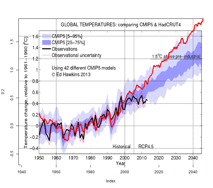
Figure 2. Overplot of UK Met Office CMIP5 contribution on CMIP5 distribution (from Ed Hawkins here.) Slight extension of HadCRUT4 to current (thin black).
Here is another overlay of the UK Met Office CMI5 contribution onto graphic from Stott et al 2013 shown at Hawkins’ blog here. I’ve extended the current temperatures from the 2010 shown in the original graphic. One of Hawkins’ readers had asked him to do so, but Hawkins begged off saying
Couple of thoughts – firstly I think the observations would still be inside the dashed lines, just, but I didn’t make the plot so I can’t add them to check.
I didn’t make the original plot either, but it’s not that hard to an overlay (see code below.) With the updated data, observations are outside the dashed lines.
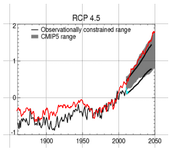
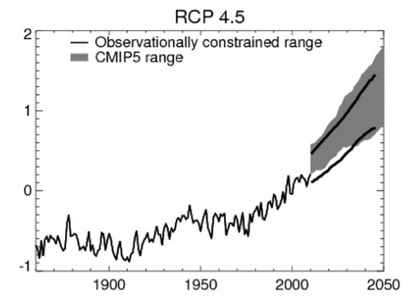
Figure 3. Overplot onto http://www.met.reading.ac.uk/~ed/bloguploads/stott_2013.png. Code is as follows (retrieval of HadCRUT4 is done elsewhere.)
loc="http://www.met.reading.ac.uk/~ed/bloguploads/stott_2013.png"
dest="d:/temp/temp.png"
download.file(loc,dest,mode="wb")
imgs=readPNG(dest)
par(mar=c(1,1,1,1))
plot(0:1,type="n",xlim=c(1850,2060),ylim=c(-1.2,2.4),xlab="",ylab="",axes=FALSE)
rasterImage(imgs,1841.2,-1.38,2064,2.37)
abline(v=seq(1800,2050,50),lty=3)
abline(h=seq(-1,2,1),lty=3)
points(2010.5,.217,pch=19,col=2)


77 Comments
Not sure if this is off-topic – if so, please snip. Way back in the mists of time (about 10 or 15 years ago) the temp in the 30s was about equal to the temp in 1998. How did it get to be a half degree cooler comparatievely?
Steve: In the US, not the ROW. For the purposes of this post, I prefer not to litigate temperature data, which has been discussed elsewhere.
not “about equal”, but much higher.
http://stevengoddard.wordpress.com/data-tampering-at-ushcngiss/
The hindcast as shown/calibrated matches very well from about 1960 to 2000, so agree that calibrating from 61-91 vs. 71-01 will not make a material difference.
Steve: agreed. HadCRUT comes originally in 1961-90 anomaly and that’s why I used it. ALso it gives better separation from recent period.
The main problems with the models are clear: they overestimate the impact of CO2 and underestimate natural variability. That makes that the change in the period 1900-1945 with little CO2 increase is underestimated and that of the period 1976-2000 is fully attributed to CO2, while the same natural variability (ocean oscillations, solar,…) may have been at work in both periods…
“The main problems with the models are clear: they overestimate the impact of CO2 and underestimate natural variability. ”
That’s not at all clear. Mismatches can result from any number of causes: getting the forcings wrong. Missing some physics. get some physics wrong. combinations of the former.
All you know is that the model doesnt match observations, and technically, you have to rule out observation error as well. so you dont even know the model is wrong.
Nothing follows from a mis match of models and data. zip. well, more study follows, but on the logical front you have many branches from a the observation of a mis match to the diagnosis of the cause.
I wonder how good the match would be with the older bucket adjustments?
Spence_UK:
HADCRUT3 would perform slightly worse than HADCRUT4:

The golden rule of climate science is to adjust the data so that it better matches the models.
Thanks for the link, Bob. The two are very similar, although the most obvious difference, in the 1950s, would help the match – but only really around that decade. Prior to the 1940s, the model appears to hindcast a very flat trend, and the strong increasing trend in observations is completely missed.
Part of the problem with anomalies is the ability to select an anomaly that looks better. I suspect (although haven’t tried it) that placing the whole model curve lower (e.g. by creating the anomaly on the entire 20th century) would make the match look visibly more appealing, even though it technically doesn’t change the quality of the hindcast at all.
Although I dislike relying on trends, these are what we are told by climate scientists are the best thing to check, and it seems clear that the trends are hindcasted quite poorly pre-1940 and in the most recent times.
The small blue line of 2012 HadGEM3 Decadal is very hard to distinguish at the end of the black line. A lighter blue or another color differing from black might be clearer.
Thankyou!
What is that blue line again? It is in the future.
Modeling is my line of work, and the only way to claim success for this kind of work, is if your notion of success consist of cementing the notion that we are in position at all to be trying to predict future climate change.
You have a model with virtually endless set of not-too-terribly well constrained parameters, but you can even fit a linear trend?
Seems like some key parameters/interactions are still missing then.
“In the Met Office, we have the biggest supercomputers in the world, which are great at back-projecting climate, but their projections of climate into the future have all been inaccurate.”
Graham Stringer, Member of Parliament
“But reproducing the known change of global temperature is 20/20 hindsight. It’s not a strong test of predictive skill. That experiment is called a hind-test. The real test is a fore-test, predicting future evolution. Only then can one be confident that models haven’t been tuned to match observed behaviour. That’s tantamount to a double-blind test, the standard rigor required in clinical trials of pharmaceuticals. Neither the patient (the model) nor the clinician (the guy running the model) then knows the outcome.”
Dr Murry Salby
Over to you, Dr. Betts:-)
Are computer models reliable?
Yes. Computer models are an essential tool in understanding how the climate will respond to changes in greenhouse gas concentrations, and other external effects, such as solar output and volcanoes.
Computer models are the only reliable way to predict changes in climate. Their reliability is tested by seeing if they are able to reproduce the past climate, which gives scientists confidence that they can also predict the future.
But computer models cannot predict the future exactly. They depend, for example, on assumptions made about the levels of future greenhouse gas emissions.
From Met Office Publication: “Warming. A Guide to Climate Change” (dated 2011-10-24)
It seems clear that the reader is meant to understand from this that, were it not for the need to make assumptions about future greenhouse gas emissions (plus?), models could “predict the future exactly”.
Re: Martin A (Jul 20 06:16),
But, as I’m sure you’re aware, reproducing a past climate is not difficult given the number of tunable parameters in any climate model created to date. Therefore it shouldn’t give scientists or anyone else any sort of confidence whatsoever. That such a statement is made in a publication less than two years old should be all that is needed to prove that the Med Office doesn’t understand either models or climate.
The Med Office?
At this rate they should keep taking the tablets.
Re: Richard Drake (Jul 20 09:16),
Since turn about is fair play, could you tell me what you meant the bolded words to read?
There’s no doubt that the models can’t solve the fundamental questions. They can solve simplified versions of them, but if they actually tried to run the models without cheats of one sort or another, they just blow up. Warmers can’t admit this, however, or the whole house of cards falls down. If there’s anyone here who actually believe what Ms. Slingo says, please speak up so we can try to set you straight.
Sorry, should have read simply do they. Here.
“The Tacoma Narrows bridge was also built using very fundamental laws of physics, but that doesn’t mean it is still standing today.”
Actually not. Missing physics: aeroelastic flutter, also the designer had an untested theory.. cant recall the cite to his paper.
Dave46
You might think that. However, please take note of the words of Professor Julia Slingo, the Chief Scientist of the Met Office:
“I think what people find difficult to understand is what is this thing that we call a model? Well, it’s a huge computer code and it’s about solving the very fundamental equations of physics which describe the motion of the atmosphere, the motion of the oceans, how clouds form, how the land interacts with the sun’s rays, how it interacts with rainfall and so on and so on.
So what these models are is hundreds and thousands of lines of code which capture and represent our best understanding of how the climate system works. So they are not in a sense tuned to give the right answer, what they are representing is how weather, winds blow, rain forms and so forth, absolutely freely based on the fundamental laws of physics.
(Met Office: Ask the expert – Prof Julia Slingo, dated 2009-12-16)
They have the necessary resolution to ‘solve the very fundamental equations of physics which describe the motion of the atmosphere, the motion of the oceans, how clouds form, how the land interacts with the sun’s rays, how it interacts with rainfall and so on and so on’ do you they, Martin?
Julia Slingo:
” … it’s a huge computer code and it’s about solving the very fundamental equations of physics which describe the motion of the atmosphere, the motion of the oceans, how clouds form, how the land interacts with the sun’s rays, how it interacts with rainfall and so on and so on.
So what these models are is hundreds and thousands of lines of code which capture and represent our best understanding of how the climate system works. So they are not in a sense tuned to give the right answer, what they are representing is how weather, winds blow, rain forms and so forth, absolutely freely based on the fundamental laws of physics.”
————————————
Gobbledeygook. WTF does “absolutely freely based on the laws of physics” mean?
How can a computer program “solve the very fundamental equations of physics”? What on earth does that even mean?
I am no scientist, but have written a lot of words which were later regurgitated by politicians who often knew little or nothing about the subject.
My career would have ground to a screaming halt if I had ever proposed words such as these. This is the Chief Scientist speaking? Oh, boy.
Slingo:
“[The models] represent our best understanding of how the climate system works.”
Quite. Perhaps a bit of “quiet time” for the scientists would be in order.
James, I’m thinking the Naughty Step, for at least a decade.
Julia Slingo’s garbled comments are just astonishing. How can someone get a higher degree in science when they make statements like:
“it’s a huge computer code and it’s about solving the very fundamental equations of physics …”
I have no scientific qualifications whatsoever, have not had the benefit (as she has) of working in the world of science, but am confident in saying that her statement is nonsense.
The Tacoma Narrows bridge was also built using very fundamental laws of physics, but that doesn’t mean it is still standing today.
Joanna
Gobbledeygook. WTF does “absolutely freely based on the laws of physics” mean?”
I think Slingo would like you to understand that it means they built their models according to the laws of physics without any adjustment to ensure they gave the desired results.
As Steve says, with immense tact and diplomacy, this “suggests a certain amount of salesmanship” on Slingo’s part.
Steve:
Martin A and daved46 have made the general argument against GCMs, a point with which I have always agreed and is the most fundamental component of my ‘attribution scepticism’, to borrow the taxonomy of James Painter.
But what a dull world it would be if we didn’t also have Steve’s sardonic commentary on a welter of unimpressive details. Met Office salesmanship, meet your doom, for the best possible reasons.
Well I for one am extremely grateful for Steve’s commentary, that “Met Office salesmanship” is having a dire effect on people’s lives here in the UK. The Government is using it as an excuse to ‘combat climate change’ and hike energy prices up though they are being extremely dishonest about the effect of their policies.
“Why you’ll be paying £3,250 extra for gas and ‘leccy in coming years
It’s not ‘gas prices’: It is the Will of The People, says Psychohistory prof
By Lewis Page, 19th July 2013 ”
http://www.theregister.co.uk/2013/07/19/energy_firm_heres_the_truth_on_how_greengov_cranks_up_your_bills/
An excellent and revealing article highlighted at Bishop Hill’s blog.
I don’t see the point in running hindcasts at all. You could always tweek this or tweek that parameter until your model approximates the station data. Likely the parameter you are tweeking may not be the one that has caused the effect in the first place. The modelers have no idea what really caused the 1940s to 1970s dip in temperature. I read that they assumed aerosols were one cause. The main assumption is that increased levels of GHGs has driven the 20th century uptick in temperatures, not a natural climatic rebound from the effects of the LIA. Since CO2 levels are increasing nearly linearly,
the future temperatures must also do the same. (With hindcasts you can put in some
fudge factors for the occasional volcanic explosion, etc. ) As a modeler, although
not in the field of climate, of 30 years experience in running very large computer simulations, I find the task of trying to model future climate very daunting. You can only model what you understand, and as Don Rumsfeld said, there are things you don’t know, and things you don’t know that you don’t know. I would take a different approach, much like Dr. Lindzen, to mainly try to do a simpler model of the sensitivity of the climate to changes in GHGs, although in no way is simple. A half-degree C divergence in the models just a few years out raises questions.
I don’t see the point in running hindcasts at all. You could always tweek this or tweek that parameter until your model approximates the station data”
I have a Lotus 1-2-3 spreadsheat that produces perfect hindcasts.
However, its forecasts are as useless as an ashtray on a motorbike.
sheet
It’s a lookup table of past values.
Fair enough, but there was no need to swear to start with 🙂
My take—the reconstructed temperatures are not reliable enough prior to 1950 to draw many conclusions about whether the models are reliable or not. Beyond that, there is a substantial amount of tuning in the models.
I think the good “agreement” between a particular model and data during the backcasting period is more of a statement that somebody “worked hard” to tune their model, and possibly had more money and other resource to get their model “look good”.
(Forecasting skill would be the appropriate place to test the validity of the models.)
Carrick wrote “(Forecasting skill would be the appropriate place to test the validity of the models.)”
Another way to test validity would be to match enough data sufficiently closely that the match can’t be due to overfitting, because (roughly) the number of independent observations being matched is much larger than the number of degrees of freedom available for tuning to improve the fit. (The “number of degrees of freedom” notion can be refined in various ways, e.g. Vapnik-Chervonenkis dimension.) I would guess (indeed, guess somewhat wildly because I’m ignorant of lots of things like measurement uncertainty and observed correlations at different time and spatial scales) that we already have enough data to convincingly check a realistically complex model if the model extended its predictions down to the detailed level where we have lots of data. (Detailed data like individual and cross-correlated statistics of local stations and individual satellite pixels.) In principle it might even be possible to use recorded weather observations to work backwards to estimate important unrecorded inputs like particulates and land use, and *still* get a mathematically convincing can’t-be-overfitting fit. In practice, given the heroic approximations needed to model a system as complicated as the earth, it seems unbelievably unlikely that anyone will be able to do that, so probably a climate modeler’s best bet is to stick to predicting a few degrees of freedom that are easy to overfit, then pound the table about how closely the hindcast matches (a few degrees of freedom in) historical data. But if tomorrow a superadvanced civilization sent us a superfast computer and a model that actually captured the physics, I think we could reliably recognize the model as good (and not explainable by overfitting) with a few months of analysis of very detailed hindcasts, without waiting for decades to see how it does on forecasts.
I’ve often wondered why we don’t see Vapnik-Chervonenkis analyses of the existing simulators. That would at least put a bound on the degree of tuning involved.
Carrick, the models are tuned but we know that models can’t simulate most metrics even over that past three decades, including sea surface temperatures:
Precipitation over land and oceans:
Daily Tmax and Tmin and Diurnal Temperature Range:
Hemispheric sea ice area:
Etc.
Regards
Climate models have been used for forecasting and the results are terrible (Dave Williamson).
Syvie Gravel’s manuscript shows how quickly a forecast model goes astray because of the dominant
error (boundary layer nonsense). They are only brought back to reality by inserting new obs every
6 or 12 hours – a process known as updating (a tuned blend of obs and model data).
Jerry
Jerry, I’m very interested in this. CAn you provide a reference of link for Gravel’s paper? You may remember me from Boulder around 1978 or so. I went to one of your NCAR seminars on sound wave filtering I think.
I’ve since been working on Navier-Stokes and we have found that eddy viscosity such as is used for boundary layers is not very accurate. It’s usually overly dissipative.
Best,
Dave Young
Can someone clarify the meaning of hindcast please because this looks like another word hijack and meaning twist.
I expect it to mean forecasting with time reversed where in this context take conditions today and forecast/model from then backwards.
I suspect the meaning used is nothing of the kind but merely taking some past point in time and then forecasting (ie. forwards in time) from that point, which is not hindcasting.
Forecast with withheld known data is a normal development technique which I assumed was entirely normal in climatic work, yet the word seems to have appeared often recently as though this is new.
An old Chinese saying goes: “Those who have knowledge, don’t predict. Those who predict, don’t have knowledge. “
Overfitting
XKCD
That was supposed to point here …
http://xkcd.com/1122/
And yet I tell you: nobody will produce a cartoon on overfitting as good as that for a very long time.
Hi Steve – I have a comment on
“We often hear about the supposed success of current GCMs in hindcasting 20th century from first principles.”
The GCMs are not first principle models. Except for the pressure gradient force, advection and gravity, the models are constructed with parameterizations that are always using parameters and functions that are tuned [usually from a very limited set of observational data during “ideal” conditions, and/or from a higher resolution model with its own set of tuned adjustments).
Then the parameterizations are applied to situations for which they were not tuned.
I discuss this issue at length for mesoscale models (and the same restraint exists for GCMs) in my book
Pielke Sr., R.A., 2002: Mesoscale meteorological modeling. 2nd Edition, Academic Press, San Diego, CA, 676 pp. http://cires.colorado.edu/science/groups/pielke/pubs/books/mesoscalemodeling.html
Pielke Sr, R.A., 2013: Mesoscale meteorological modeling. 3rd Edition, Academic Press, in press
The same issues of tuning of parameterizations apply to the all other components of the climate models (i.e. in the representation of physics, chemistry, and biology in the oceans, snow and ice, soil, vegetation, etc).
I also recently documented the failings of the CMIP5 hindcast runs in my guest post at http://www.climatedialogue.org/are-regional-models-ready-for-prime-time/.
Best Regards
Roger Sr.
It’s very nice to see Roger Sr on CA. On a more anecdotal note, I’ve just found this from an interview of James Lovelock by Leo Hickman in the Guardian in March 2010:
“We haven’t got the physics worked out yet.” But the folks at the Met Office don’t always say that as clearly as they might publicly, do they?
Umm, Gerald,do you realize who you are addressing your comment to?
I’ve added an update showing the UK Met Office contribution to IPCC AR5 against a couple of graphics from Ed Hawkins’ blog. Hawkins’ blog has some interesting posts and is worth a visit.
The planet’s at stake and it’s this volunteer who takes time (in both senses) and becomes first to witness such naughty observations. Satisfying moment.
Broad-brush template for func CS_tm_postLIA_HindcastProjection
/*REM//apply explicit casting on unarchived data where convenient e.g. (established physics) on (adjusted as appropriate GAT) \\UNREM*/
switch (maraschino as public)
case maraschino.startyear==1920 to maraschino.endyear=1930;
call AdjustParametersToFitFunding(maraschino );
break;
…// repeat and adjust parameters as required for correct conclusion
Broad-brush template for func CS_tm_postPresent_HindcastProjection(*Forecast)
Forecast=SettledForecastFundingFunc(Random(0.97*CONSENSUS));
Call CS_tm_postPresent_HindcastProjection(Forecast)
Darn – it doesn’t compile but, at least, it does comply.
SteveM, while looking at an average scenario model result when compared to an observed series , such as you show with RCP4.5 here, is revealing, some readers here might think that there is one or a few magic model runs that get it “right” vis a vis the observed record. To that end I have taken all the difference series from all the RCP4.5 model runs minus the GHCN observed series, then did a breakpoint determination that divides all the entire difference series into linear segments, then regressed those segments against time and finally summarized those results showing the number of significant trends in the linear segments and whether the trends are negative or positive for each model run GHCN difference pair. I also include the number of years in each linear segment.
I’ll post the results at this thread with a link to the tables showing the results. I can say right now that no difference series of RCP4.5 model runs versus GHCN has no breakpoints.
Slightly OT, but I was at a symposium recently where a very warmist climate scientist presenter had several digs at the deniers (yes, that branding was used). One of their points was, in countering the discrepancy between models and actual temperature record, that only 5% of the difference could be attributed to the models themselves. I hadn’t heard of this before, has anyone here?
I don’t think that such a statement makes any sort of scientific sense. What was the other 95% of the difference attributed to?
I get the distinct impression that the presenter might have made a rookie misinterpretation of a confidence interval or a statistical test.
The UK Met Office HadGEM2 AOGCM has an exceptionally high climate sensitivity (ECS = 4.59 K, topped only by the MIROC-ESM model at 4.67 K), and the highest TCR (2.50 K) of any CMIP5 model analysed, per Forster et al 2013, JGR. That would account for its very high projected future warming.
At the same time HadGEM2 has a low radiative forcing for a doubling of CO2 concentrations (2.93 Wm-2, c/f 4.26 Wm-2 for MIROC-ESM, a mean of 3.44 Wm-2 for CMIP5 models analysed, and a generally accepted figure, used in AR5 WG1, of 3.71 Wm-2). HadGEM2’s sensitivity to forcing is therefore much higher than MIROC-ESM’s, at 1.57 vs 1.10 K/Wm-2 for ECS and 0.85 vs 0.52 K/Wm-2 for TCR.
HadGEM2 also has high negative aerosol forcing level, which would have had a depressing effect on its simulated change in global temperature between 1950 and 1980 or so, when aerosol loading rose rapidly. As a result of its high aerosol cooling, HadGEM2’s net forcing change from pre-industrial to 2010 was only 1.0 Wm-2, under half the estimated change per in the leaked draft AR5 WG1 report. That explains why HadGEM2’s hindcast rise in global temperature over the 20th century is unrealistically low. But under the RCP45 scenario, aerosol loadings are projected to fall from now on. So simulated future global temperature changes by HadGEM2 will fully reflect its very high TCR.
There is no doubt that HadGEM2 is an outlier model in terms of its simulation of, and response to, radiative forcings, however good it may be at simulating weather patterns in the short term .
So there are two categories of uncertainty in modeling future climate.
1. Sensitivity of a model to forcing – the code in the model
2. What the modeler has predicted future forcing(s) will be – CO2 concentration, aerosols, land use changes etc.
An engineer can design a car and predict what its fuel economy numbers will be for a given set of conditions. Separately, an engineer can predict but can’t know under what conditions (forcings) the customer will use the car. “Your mileage may vary.”
Thanks for this Nic, I was hoping someone would post on the “why.” If I am interpreting what you wrote correctly, you are saying that hadGEM2 had high sensitivity to non-CO2 radiative forcing but low sensitivity to CO2 radiative forcing? The twin uses of “climate sensitivity” in the vernacular makes it a bit confusing. At any rate, a consensus seems to be forming that Trenberth’s missing heat was blocked by aerosols, but the heat is still coming as aerosols decline.
“you are saying that hadGEM2 had high sensitivity to non-CO2 radiative forcing but low sensitivity to CO2 radiative forcing?”
Almost right. I am saying that hadGEM2 has high sensitivity to non-CO2 radiative forcing (in W/m^2) but lower sensitivity to CO2 doubling than one would expect given its sensitivity to non-CO2 forcing”
Aerosol load and influence is the largest tuning button besides cloud influence that they do use in models. If you compare the human emissions of SO2 with that of the Pinatubo, then the maximum influence is a 0.1 K global cooling if taken into account the short (4 days) residence time of human aerosols in the lower troposphere before raining out against the 2-3 years residence time of the Pinatubo aerosols in the stratosphere. Since the 1990’s there is a huge decrease in the Western world and a huge increase in S.E. Asia, which nearly compensate each other. Despite that there is no more warming downwind the largest sources in Western Europe than upwind. And all NH oceans show more heat content increase than the SH oceans, if taken into account the difference in area, despite that 90% of all human aerosols are emitted in the NH…
What I find fascinating in reading this thread and the earlier, related ones,is the extent to which Phil Jones is being proven correct. The more data and code become available the greater the extent to which our host and a growing host of others are proving the GCMs, the stats, the data etc. are, to be polite, questionable. In other words they are just looking for things that are incorrect (often indefensible!)and finding them.
Well, good! I’ve been asking people for quite a while now: What makes you think that the models are good enough to predict a century’s worth of surface temperatures? If they aren’t, the only way that all the current models do that must be through overfitting. It’s a sign of bad model design.
The only counter-argument, that they are based entirely on physics, not on tuning, is (I think) disproved by the fact that their forecasts have almost immediately shown to be much worse than their hindcasts.
It’s a good sign if they have dropped the bad requirement of tracking the twentieth century’s temperatures, and decided to focus on predict ing a much larger ensemble of climate variables for a much shorter time period. Among other things, we’ll be able to check the forecasts much much faster. Under the old system, you got _one_ new data point per month.
In the 1960’s and 70’s there was a lot of research on optical character recognition, in the hope of constructing automatic systems to read postcodes, figures on cheques and so on.
When tried in the field, the performance was invariably much poorer than lab tests had predicted. It slowly dawned on investigators that the fallacy was “testing on the training data”, which lead to unrealistically good estimates of performance in terms of error rates and so on.
I think the same fallacy applies to climate models. Observations have been used to “parameterize” parts of the model where physical knowledge is lacking. Hindcasting then evaluates the model’s ability to reproduce climate over the same period used to obtain the parameterization data.
Deja-vu. It’s testing on the training data all over again.
Are climate modellers really using the same data to determine parameters and to demonstrate goodness of fit? If it is, then they are either being incredibly stupid, or are setting out to deceive. The golden rule is to calibrate parameters using one set of data, and validate using an independent set of data.
They claim they are not (“it’s all based on physics, not tuning.”). However, if we’ve learned anything from Machine Learning, it’s that data snooping and overfitting are incredibly hard to avoid. And these models are based on earlier models, and all of them had to match a century of surface temperatures or they went back and fixed them. I would have thought it’s going to be virtually impossible to track down any overfitting at this point. It can, however, be verified by failure of the models to predict out-of-sample correctly.
I was just reading Harry Collins on the detection of gravitational waves. That community obsesses over the possibility of the “trials factor” exaggerating their significance levels. So they use blinding procedures to prevent ex post, ad hoc adjustments and many of them only want to report five-sigma results as a further safeguard. Collins argues that their conservatism may have gone too far, but it is a striking contrast with the apparent norms in climatology.
Steve, could you put Ed Hawkins’ blog on your blogroll, please.
In a further look into the comparison of the modeled runs from CMIP5 and the Observed series for the historical period, I took difference series of the RCP4.5 series with 106 runs with 42 different models and the GHCN observed series from 1880 to May 2013. The series were anomalies for the period 1880-2013 May for the global mean monthly temperatures as collected at KNMI.
The 106 difference series were then partitioned into linear segments using the breakpoints function in R and those linear segments regressed against time to estimate the trend slope and t.values. The results are given in 2 parts in the linked tables below along with the length in years of the linear segments. The summarized results showing the total number of significant trends and the number positive and negative trends for each model/GHCN difference pair is part of a table in the third link below. That same link includes a table identifying the model code I used with the models’ official names.
In no cases were the linear segments of the difference series greater than 5 (breakpoints greater than 4) or less than 3 (breakpoints less than 2). Examination of the tables shows that there are many linear segments for relatively long periods of time that have significant trends both negative and positive. The summary in the table in the third link below shows that the total significant trends (absolute value of t.value less than 1.96) for each difference series is most often 5 and only less than 3 three times. The difference series graphs (not shown here) show for those series with less than 3 significant trends: MRC minus GHCN, with one, actually gives a large negative trend over the entire 1910-2013 May period; CMS minus GHCN, with two, gives a very steep upward trend 1880-1910 and then steeply downward from 1910-1940; FIO_2 minus GHCN, with 2, gives essentially the same pattern as CMS minus GHCN.
Notice also that models that had multiple runs could have very different numbers of significant trends and signs of trends for the runs. Also note that these models are essentially hindcasting over most of the 1880-2013 time period.
I judge that based on these significant and prevalent differences over long periods of time a comparison of the observed and modeled series is perilous and without a lot of meaning until the models reasonably well emulate the observed within the historical instrumental temperature period.
I also think that, if one is not restricted to modeling these intermediate periods reasonably well in tune with the observed record, it becomes an easier task to apply adjustments to the models to obtain agreement over longer periods of time.
I would think also that the models would be required to better approximate the natural fluctuations of the observed climate before we can determine how well the models are getting the response to anthropogenic forcings correct.
I should add that when a difference series between GHCN/GISS and GHCN/HadCRU4 pairs are presented for breakpoints determinations there are breakpoints: 2 for the first pair and 3 for the second. In a perfect world I suppose we would expect to see none and the fact that we see some provides fodder for further examination of the observed series. Those differences series between observed series have linear segments with trends averaging 0.024 degrees C per decade which can be readily seen when compared to the GHCN RCP4.5 model difference series trends to be much lower.
The GHCN/Model difference trends had an average trend=0.105 for the individual pairs with a standard deviation of 0.027. If we consider the Observed pair differences as a baseline then we can say that the diminished trends in the Observed pairs is very significantly different and smaller than the GHCN/RCP4.5 pairs. The only GHCN/model pairs out of the 2 sigma range were those for the model MRC at an average trend = 0.037 and IN at an average trend = 0.048.
It should also be noted from my previous post here that the 2 models that performed closest to the Observed series in consideration of difference series trends with GHCN were also the models with the lowest of the 106 RCP4.5 model runs for trends in the 1970-2013 May time period. The MRC model run had a trend of 0.080 degrees C per decade while the IN model run had a trend of 0.106 which compares to the GHCN trend over the same period of 0.161. This finding shows that while one can look at the breakpoint defined segment trends to determine how well the models emulated the observed temperature series it is not sufficient in determining differences. While IN and MRC perform best when comparing the linear segment trends, those models show much less warming than the observed series do in the period were AGW should show its biggest effects.
I have to keep harkening back to the importance of what the model/Observed comparison shows on a measure of how well individual models and model runs can emulate the Observed series rather than “best” models or an ensemble average. My analysis shows that none of the model runs, or at least for the CMIP5 RCP4.5 scenario runs, get it “right”.
I asked Prof Richard Betts (Met Office) when the model suggest a high rate of warming will start up again (and could not, get answer) we did agree that current rate of warming much lower than 0.3C on average required to hit low end 2040’s projections..
Richard and I on video, filmed at the Met Office here: (neither of us is Brad Pitt)
http://www.myclimateandme.com/2013/05/07/when-barry-met-richard-our-first-poll-winner-comes-to-the-met-office-2/
as they paid expenses, train, taxi’s, lunch I guess I’m now in the pay of ‘Big Climate’ never to be trusted by a sceptic again (my little joke)
Barry,
THAT PAGE COULDN’T BE FOUND! (apologies for the caps, which are myclimateandme’s).
Have they junked it, or is there a typo somewhere? Looks like the former, as it was formerly available on Facebook, but is now no longer. Do you have another link?
@Mosher July 21 3:19pm
Your quote:
If it’s not tested, it’s an hypothesis, not a “theory”
Global warming has been on “pause” for 15 years but will speed up again and is still a real threat, Met Office scientists have warned.
Thanks Martin.
So they were aware in 1997 that temperatures might remain stable for 20 years from that moment but forgot to mention this to the general public? Or was it later that this realisation hit them? When exactly?
Were they aware that most of their models would be invalidated by a pause as long as 20 years? Did they realise, in other words, that their models were already invalid, based on this stated ‘awareness’. At what point were they aware of this?
Met office models predicted the warming standstill.
(Although it was only after 15+ years of standstill that it was apparent to the Met Office that their models had in fact predicted it.)
Martin, what I find interesting and at the same time a bit puzzling is that we have the 2 headed explanation of the recent pause in warming: 1) we are told that the models can show longer duration pauses in warming of the length of the recent pause and then 2) we are told that the recent warming pause is caused by the deep ocean taking up more heat than it had earlier.
What is not made clear is whether the models “know” about the deep ocean napping and then awaking to heat uptake. I doubt very much that the model excursions that on rare occasions will show 15 year level trends are related directly to changes in deep ocean heat uptake. What do you think?
I have been giving evidence to show that the models and the observed temperature trends can be significantly different over periods of time longer than 20 years. We can debate the issue of level trends of 15 years in models but that is a rather rare event and is rather beside the point of how well the models emulate the observed temperature trends.
One Trackback
[…] https://climateaudit.org/2013/07/19/met-office-hindcast/#more-18211 […]