Both in climate blog world and the financial world, there has been much talk recently about the interaction of models and data distributions. Linear regression models assume normal distributions. What happens to models when the data distributions don’t meet the assumptions. Sometimes it doesn’t matter much, sometimes it does. But it seems like an important thing to study.
The usual relaxation of white noise assumptions for residuals (and the one used in Mannian studies) is low order red noise. As so often in Team studies, this is asserted rather than proven. It didn’t hold in MBH98 and many of the “new” proxies in Mann et al 2008 depart from this assumption even further than before.
There are a variety of graphical techniques for showing different time series properties. Applied statisticians (as opposed to climate Teams) emphasize the need to examine data graphically and it’s something that I do. I do hundreds of plots and only illustrate some here. Willis has also been looking at the proxies graphically and has a post on the way, from the same sort of perspective but handled a bit differently, so keep an eye for that.
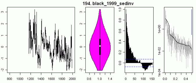
As a start, I’ll show 4-panel plot for two sediment time series, with each plot showing left to right – the time series on a common scale 800-2000; a violin plot of the distribution (this is a sort of histogram); an autocorrelation function out to lag 150; a spectrum of the scaled series again on a common scale. I’ve done these analyses on the period prior to the 20th century so that possible 20th century anthropogenic impact is not included in the distributions and spectra.
In these two cases, the distributions are quite different with the paleosalinity series being rather unsymmetric, and both have noticeable autocorrelation. I’ve uploaded similar plots for all the sediment series in this directory. These ones are in no way “wild” within the group; actually, the first one is relatively “tame” and this is one of the reasons that I’ve illustrated it here.


Now I’ll show similar plots for white noise, low order red noise (rho=.375) and a random walk (this one spending time in the negative half). White noise and low-order (Mannian assumption) red noise have very symmetric violin plots, decorrelate very rapidly in the ACF and have little low-frequency in the power spectrum. The random walk decorrelates very slowly and has an asymmetric distribution (random walks nearly always spend their time on one side or other of the 0-axis.) The salient point is that these two sediment distributions (like the others as well) do not fit the assumption of low-order red noise.


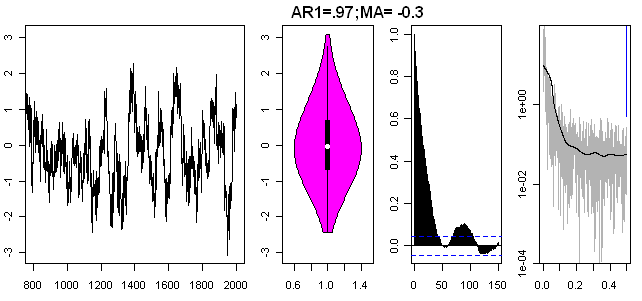
What sort of assumptions are needed to yield simulations that look sort of like these series? For the Black sediment series, here is a corresponding plot using AR=.97 (!) and MA=-0.3 (the combination of high AR and negative MA in this range is a method that I’ve experimented with in the past.) This yields a simulation that visually looks sort of like the Black sediment series. But you’re now dealing with series with much more troublesome statistical properties than a low-order AR1 series.

The fracdiff package has some nice simulation tools as well. The parameters for the Black series under fracdiff are d=0.48 (very close to the top level of 0.5!), ar =0.5 and ma=0.04. Here’s a realization from fracdiff.sim (using 3 parameters only.)

In our simulations of the North American tree ring network, we used a more awkward simulation method which used the entire ACF functions. This has resulted in some carping by Wahl and Ammann, though they conceded that the method yielded realistic looking time series. If we were doing this again today, I’d simulate these results using fracdiff as above. It’s not something that makes any difference to the effect discussed in MM05a, as the bimodel HS distribution reported in MM05a holds even with simple AR1 and the longer-persistence models simply spread out the bimodal lobes a bit.
The big problem with these series for statistical analysis is that they are much closer to random walks (AR1=1) than to white noise (AR1=0) and these sorts of series are highly prone to spurious regression. Tests designed for white noise (and relaxed slightly to include low order red noise) don’t work. Not that that deters Mann et al.
Of course, it’s hard to imagine real life events occurring which were unanticipated by models, isn’t it?


13 Comments
Steve, for the GRL paper we used ARFIMA, where the FI= fractional integration. Isn’t that the same as fractional differencing?
Can you run a unit root test on these series? I’d say a de-trended Phillips-Perron would be the appropriate one. With ACF’s like that they might be indistinguishable from integer-integrated series.
It is not surprising that a hydrological series has strong persistence. The only way to justify using the series in a regression model without a transformation to make it stationary would be if it is included in a group that fractionally cointegrates to yield a stationary linear combination. Otherwise you are absolutely right that an AR1-type noise benchmark is inappropriate.
Re: Ross McKitrick (#1),
One of the odd things about the time series that Steve is talking about (which exhibit d=0.50-\epsilon) is that they appear to correspond to stationary ARFIMA models — but just barely.
Why Mother Nature chooses to reside right there is a good question. I look to Koutsoyiannis…
Here are plots for 2 series which are of current interest. These series are about as fractional as they come. Coefficients under fracdiff of d=0.4984879, ar= 0.8429964, ma=-0.3831452. These series are a disaster for regression methods. Now go see Jeff Id on these series.
Ross, the difference is just in the simulation algorithm. The hosking.sim algorithm uses the entire ACF and people have worried that this method may have incorporated a “signal” into the simulations. It’s not something that bothered Wegman or NAS, since the effect also holds for AR1, but Wahl and Ammann throw it up as a spitball. Fracdiff is a 3-parameter simulation and is a cleaner simulation that avoids the spitball.
False. Or ambiguous. The assumption of normal distribution only concerns the residual and not the time series (data). It is a common mistake. It is true that it is generally difficult to obtain normal errors if X and Y are not normal, but it is not impossible.
To prove your point, you have to look at the residuals, and not to X.
Re: Ignatus (#4),
Hmmm! According to http://www.uoregon.edu/~robinh/gnmd03_basics.txt linear regression and ANOVA models are those which assume independent and normally-distributed random variables with constant variance. Maybe you’re thinking of generalized linear models (GLMs) that exist for regression-like modeling of data which do not assume a normal distribution.
#4. In this particular example, both situations apply. Consider any temperature history that you can imagine – including any of the Mann 2008 reconstruction variations, together with the implied estimate of various proxies. The residuals are the difference of two very unlike series and, if one of the two series is close to a random walk and one is low order red noise, then the residuals are going to be offside. I thought that this was implicit in how I expressed things, but, if not, that’s surely the case.
#6. I think that I mentioned a while ago that Mandelbrot himself studied the Hurst parameters of a wide variety of climate time series, including sediments and U.S. tree rings.
The answer from Kaya, might not work to Maya.
==============================
Steve, What I find interesting are the models – forward integration, rather than regression. Most of the model results show – more or less positive exponential growth with time. We know (I think) that they throw out all of the model runs that go negative, so you are left with random walks, leading to exponential growth that I have always assumed (but I can’t prove it) are due to roundoff or truncation errors in the model. Aggragating these runs to produce a final result assumes a normal distribution by cherry-picking only positve results.
Questions – what is the sampling resolution on the sediment series and ACF plots? You say you compute the ACF out to lag 150, does this mean 150 years?
If these plots show annually-resolved data, presumably these have been interpolated from coarse resolution series, and are somewhat artificial in nature(?) According to the ACF plots, one could presumably obtain quasi-independent data points by using only one of every ~70 values. Of course, this wouldn’t leave you with much to use for calibration with modern temperature records.
#4: It’s true that the OLS normal equations only assume something abuot the residuals; also maximum likelihood assumes normal errors. However Steve is talking about something different. The independent variables cannot be nonstationary in a regression model. The dependent and independent variables have to be I(0), i.e. integrated of order zero. if variables are fractionally or integer-integrated the assumptions that are necessary to use t tables for assessing significance of the slope coefficients no longer hold. If the variables are I(1) the t-states will be wildly misleading unless all the I(1) variables form a linear combination that is I(0), which is called cointegration.
Accumulation of capital is nature’s way of coping with risk inherent in a variable environment. Capital accumulation processes are Hurst process, and many of the processes Mandelbrot studied were capital accumulation processes. Tree growth is a capital acucmulation process. So is stock market growth. That’s why the patterns are everywhere – because capital accumulation is everywhere.
One Trackback
[…] instead of the dubious ARFIMA null proxies, by both the NRC report and Wegman et al. As late as September 2008, McIntyre proclaimed: The hosking.sim algorithm uses the entire ACF and people have worried that this method may have […]