I said that I post the graphic from Loso et al if someone sent it to me today. In fact, Loso et al is online here and interested parties can consult it for themselves. I don’t have time to comment on this study other than very briefly, but here are some of the key graphics.
Loso is studying a proglacial lake and, prior to showing the Loso graphics, I’d like to remind people that we’ve looked at some proglacial lakes in other locations e.g. Venezuela, Peru, Kilimanjaro and I think that interesting information can be derived from them. For example, here is a graphic from Polissar et al on Venezuela (discussed here) showing a difference in magnetic susceptibility between MWP and LIA sediments in Venezuela, which Polissar et al interpreted as showing an absence of glaciers in this location in the MWP.

Venezuela Proglacial Lakes – see http://www.climateaudit.org/?p=704
So Loso adds to this class of evidence. Loso examined 12 cross-sections at Iceberg Lake in a glacial lake, providing the following interesting diagram.

Original Caption: Figure 3. Stratigraphic sections from twelve sites at Iceberg Lake. Marked depths are distances, in cm, below the top of the section. All sites except I” were documented in outcrops exposed subaerially by stream incision in the exposed lakebed. Site I is above the most recent stable lake level and was collected with a Livingstone-type Corer. Using a combination of varve-counting, cross-dating, and radiogenic dating, we tied the sections shaded in red to a master chronology. Dating on other sections is uncertain. Note that Sites H and L do not exist—these two breaks in the lettering system divide sites visited in 2001, 2002, and 2003.
Some of these exposures could be dated. From my reading, Sites C, D, E, F, and G could not be dated. Thus, the set of cores was reduced by 5, yielding the following set of core measurements.

Original Caption: Figure 5. Well-dated varve thickness chronologies from seven sites at Iceberg Lake. Each chronology includes measurements from all laminae confidently dated through a combination of varve counting, cross-dating of visually distinctive laminae, and radiogenic techniques. For nine macrofossils found within these sections, thick bars show comparison of calibrated radiocarbon age estimates (2-sigma range given by vertical bars) with varve ages (horizontal bars). Radiocarbon data from Table 3.
Varve thicknesses were measured and averaged, from which a master chronology was obtained as shown below, with elevated 20th century values. I’ve rotated the original Loso Figure 6 below and added in a horizontal red line at the maximum from the smoothed 40-year filter version during the 1000-1200 period, for reasons discussed below.
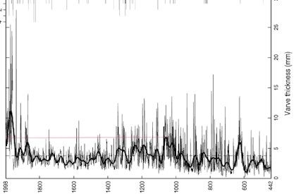
Original Caption: Figure 6. Master varve thickness chronology from Iceberg Lake. Values are averages of raw measurements from overlapping, stratigraphically correlated sections providing continuous coverage from A.D. 442 to 1998. Across all years, mean thickness (dashed vertical line) is 3.8 mm. Thick line shows the same record smoothed with a 40-yr lowpass Butterworth filter. Gray bars on right side of panel indicate numbers of laminae used in construction of master chronology, and opposite them the number of laminae excluded from each year in the plotted chronology due to evidence of turbidites, resuspended sediment, or ice-rafted debris
If one looks in detail at a blowup of the 20th century, we see what seems to be a frequent pattern in proxies: elevated values in the 1930s, with lower recent values during what is supposed to be higher recent temperatures. The Divergence Problem – Varve Style. The values at the end of the 20th century were significantly lower than the values 30 years ago.

It is certainly not correct to characterize the Loso results as presented as evidence supporting higher medieval values as compared to 20th century values. They don’t. On the other hand, it’s not a magic bullet the other way either. I’d like to see some other varve chronologies before concluding anything very much from this series. There are many assumptions and exclusions in the methodology which may or may not have biased the results. I don’t see much point in analyzing their procedures much until some other comparanda are available. The Divergence Problem, Varve Style, is very real. However plausible the rationale may be for varve thicknesses as a proxy for temperature, the apparent divergence is disquieting. In addition, and this is just an impression from the first diagram illustrated here, the appearance of the medieval section in Core J has a “quieter appearance” than the LIA sections of other cores, or for that matter, the modern cores. In the Venezuela cores, the medieval sections were also “quieter” than the modern section. This is nothing more than an impression. It would take a lot of work to really analyze what’s being done here.
I don’t exclude the possibility that well-conceived proxy studies could show to a reasonable person that the modern warm period is warmer than the MWP. However, that doesn’t mean that the Hockey Team studies have done so or , even if some future study was done correctly, that that would vindicate the Team, any more than subsequent evidence has vindicated the Piltdown Mann, using a comparison that I’ve made previously. Is Loso et al such a study? It doesn’t look like a magic bullet to me.
Updated Text – Lee has challenged the apparent contradiction between the abstract of the Loso article and the characterization of the Loso article by the Idsos. Like realclimate, the Idsos review many articles and their reviews are of unequal quality. I haven’t relied on their characterization of this or other articles. I don’t rely on realclimate’s characterization of articles.
The abstract to the article said:
Varve thickness is positively correlated with Northern Hemisphere temperature trends, and more strongly with a local, ‘ˆ¼600 yr long tree ring width chronology. Varve thickness increases in warm summers because of higher melt, runoff, and sediment transport (as expected), but also because shrinkage of the glacier dam allows shoreline regression that concentrates sediment in the smaller lake. Varve thickness provides a sensitive record of relative changes in warm season temperatures. Relative to the entire record, temperatures implied by this chronology were lowest around A.D. 600, warm between A.D. 1000 and A.D. 1300, cooler between A.D. 1500 and A.D. 1850, and have increased dramatically since then. Combined with stratigraphic evidence that contemporary jökulhlaups (which began in 1999) are unprecedented since at least A.D. 442, this record suggests that 20th century warming is more intense, and accompanied by more extensive glacier retreat, than the Medieval Warm Period or any other time in the last 1500 yr.
The “Northern Hemisphere temperature trend” used as a comparandum through linear correlation is Mann and Jones 2003, a reconstruction which I do not regard as gold standard. The tree ring chronology is Davi et al QR 2003 from the Wrangell Mountains, Alaska, a result which I’ve read and will review again in this context. Here is an excerpt from Loso’s comparandum graphic for the 1400-2000 period with the Mann and Jones 2003 hockey stick in solid, while the Davi et al tree ring chronology declines in the latter part of the 20th century, similarly to the Loso varve chronology – both showing the Divergence Problem disguised by the Mann bristlecone PC1 in Mann and Jones 2003.

Excerpt from Loso et al Figure 7, covering 1400-2000 period.
As noted by Willis, the Idsos’ characterization of the graphic focused on the closing 20th century value rather than peak 20th century values, stating:
This work revealed “a clear manifestation of the Medieval Warm Period” between AD 1000 and 1250, the peak warm-season temperature of which (”smoothed with a 40-year lowpass Butterworth filter”) was clearly higher than it was at the end of the 20th century.
In my opinion, neither Loso nor the Idsos adequately report on the Divergence Problem, Varve Style and both are too quick to claim the result as vindication for one view or another. Various CA commenters with geological backgrounds have identified many problems with interpreting the Loso results as temperature proxies.
Reference: Loso online here http://polar.alaskapacific.edu/mloso/manuscripts/losoetal2006.pdf
Update: Data ftp://ftp.ncdc.noaa.gov/pub/data/paleo/paleolimnology/northamerica/usa/alaska/iceberg2008.txt


54 Comments
re: Divergence, Varve style … 1930s vs 90s
Shh! Kvetching with those who still chant the “warmest decade of the millenium” mantra warms Mr Lee’s soul.
I have a hard/impossible time matching the 20’th century wiggles with either regional instrumental temperatures or the PDO pattern. Using the scale in hos Figure 6, it looks like the big peak is closer to 1960 than to 1930, which makes no sense to me. I guess the scale has to be taken with a grain of salt/sediment.
Speaking of sediment, it seems like sediment would compact over time, as weight is added above it. There seems to be a slope from 440 to 1900 which my layman’s view would tend to attribute to compaction rather than to temperature.
And, I wonder if compaction is nonlinear over time, meaning that recent sediment may have yet to undergo significant compaction, making it difficult to compare with deeper, older sediment.
Seems like a complicated proxy.
The year 1300 is prominent in Figure 5 and then magically disappears in Figure 6. Why so many excluded series around 1300?
#3 My thoughts as well. To add to the complications, how is run-off due to precipitation factored into the equation? Is this particular lake nearly completely enclosed within a glacier – I suspect not. Therefore I assume there are other sources of run-off and sediment.
Dave, #2
Actually, as a professional geologist my first question was exactly that. I am familiar with density measurement devices as related to core samples and it would be a simple matter to measure bulk density of the sediment core to evaluate compaction and compensate for the expected thinning effect. I will review the paper to see what correction, if any, has been done.
Given the apparent periodicity, I’d want to explore the set of possible periodic processes (or interactions of them) which the varves might be a proxy for. Is “mean global temperature” an output of a periodic process? If so, than that would indeed lead to additional very interesgting – earth shattering – discussions, at least given the current AGW obsessive context.
Well, I finally got a chance to look at the Loso et al. paper on varve thickness in Iceberg Lake. They say that varve thickness is a proxy for temperature. My research seems to support this claim, but with a curious twist. They say:
Being a simplistic kind of fellow myself, I thought “Why are they comparing varve thickness to tree rings and global temperature? What about local temperature?” So, here’s the record of my peregrinations. First, where are we talking about? The area looks like this:
The three nearest temperature stations are shown on the map, along with the location of the lake. Iceberg Lake is only about 80 km (50 miles) from the coast of Southeast Alaska. Fortunately, the three nearest stations are not far from Iceberg Lake, and it’s in the middle of the three. Here’s the temperature record:
As you can see, the three stations are well correlated, particularly in the modern period when measurements are likely to be better. Burwash, being inland, has wider swings than the two coastal stations, but they all move together.
And as you can also see, in the last century the varve thickness of Iceberg Lake is a pretty good proxy for the temperature, with just one leetle, tiny problem. Note that the scale on the right is inverted … which means that when the temperature increases, the varve thickness decreases …
Oops …
w.
In addition, I am not sure I see any trend in the temperature of these 3 stations. Do you see any trend?
Why would there be a negative correlation with temperature?
I’ve taken some time to go over this paper and as a geologist I have some major issues with both approach and conclusions.
1 – Although the Methods description says that samples were taken for grain size and bulk density analysis, only GS is reported and density is not mentioned again. I agree with Dave, compaction will probably have an effect on the apparent volume of a lamina, as the sediment would be in the range of 40%+ water at the depositional surface which is rapidly reduced to less than 20% during burial and water expulsion (some evidence of that is ref’d to as distorted beds – the 1642 event possible seismicly induced de-watering?). This would cause an apparent thinning in the varves in the past and might explain the thinnest are the oldest with an upward drift” to the MWP. He does variably say thet he cannot quantify the temp but the asserts it’s never been warmer?! There is also a curious mixture of the terms “temperatures suggested by the chronology” (P.23).
2 – The paucity of samples gives me no confidence in the uniformity of the varve thickness or relative thickness over any spacial scale. Overlap of the sections to create a The samples utilized were bunched around the post-drainage creek incisement in close proximity to the inlet delta complex of the Lumpy Glacier. The proximity to plumes of suspended sediment could easily skew any results. A look at the I section, added to the 1642 to 1850est time period shows substantially thicker varves (Fig 5). The location map Fig 2 shows the section I is at the extreme north end of the lake and would undoubtedly be expected to be thicker due to source proximity at the inlet from the Chisma Glaciers.The post-LIA shift in shoreline as the lake level dropped from 990m to 933m illustrates the “wedge” infilling from the North.
3 – The main premise of the paper is that rate of sediment influx is relative and correlatable to temperature. This is false, as Willis has pointed out. Loso et al point out that the best correlation is to that other favorite temperature proxie of climateaudit groupies, tree-ring width! I think the authors would have done better to be open to discover WHAT the varve thickness correlated to, and forgoe the repeated assertion that it MUST be temp and it’s never been warmer. Sediment is transported by water, which is introduced to the “small catchment”(P.23) via precipitation. Under a balanced system the rate of transport is not the rate of melting, ie temp, but rate of precipitation. Tvarve = fRprecip
Just as with the dendro issue, this is a precipitation proxy.
4 – My final issue (for now) is the constant assertion of current temperature blah! blah! blah! and drainage of the lake proves it’s blah!…
The basic assumption is that the glacial system is static and unchanging. I have camped at the head of a glacier exiting the Jakesfield Icecap on Ellesmere Island and listened to the growl of and watched boulder-sized sediment tossed along the marginal spillway. A huge amount of sediment is moved and I will assert that the Tana Glacier is cutting its way down and lowering the ice-dam level and has over the past 1500 unprecedented years. Glacial process is rife with unprecedent.
My last word; Willis, could you plot the same data versus precip for the local stations? It might be interesting.
I confess I haven’t read the paper yet, but there is a comment in the abstract about shoreline regression. Clearly if the shoreline is changing, then distance to the core sites from sediment sources for the summer part of the varve is changing. Hence you can in theory introduce changes in varve thickness with no changes in runoff (i.e. summer temperature). Of course mixing and matching cores with different distances from the sediment sources is probably not a good idea unless all cores are complete through the sequence which you want to analyze. In this case that does not appear to be true.
As for the winter part of the varve, where the turbidity settles out, this should be the predictable part of the sequence, but these are the finest sediments and so are more subject to compaction than the summer part (as noted above) so they have their own problem.
I can see my above post became redundant as I was writing it. No matter, I’ll make one other point regarding glaciology and climate (which has likely already been made in this forum). Glaciers take a while to advance or beat back so it’s not just the temperature of periods in which they advance/retreat, its the length of the alternating cool/warm periods that drive their history. If glacier is at its greatest point of retreat say, in warm period 2, it could be that the cold period preceding warm period 1 was longer/or colder than that preceding warm period 2. In other words warm period 1 did all the work in beating back the glacier, but warm period 2 gets all the credit, when the real culprit was that cold period 2 was lazy (not cold enough), or “booked off early” so to speak.
Yet the simplistic idea because “this is the smallest the glacier has ever been so this must be the hottest it’s been” is riddled through climate science, or is this climate hobbyist “newby” got his climate science perceptions wrong?
As for this paper, I did read it and noted that the largest portion of the sediment load must coming from meltwater off the glaciers at the head of the lake. In this case the effect of lowering the water level is to move the one of the main discharges into the lake maybe a km closer to the core site (hard to guess at the 3D image dimensions). Since they don’t know the lake level in the MWP, they can’t say whether the 20th century sediment pulse is due to unprecedented volumes of meltwater.
Roger D., thanks for the interesting post. It’s taken me a few hours to dig up the data on precipitation, but I finally got it … here ’tis:
As you can see, the varve thickness is negatively correlated with precipitation, just like with temperature.
Go figure …
w.
Willis,
It might be interesting to check precip x temp correlations as well. In SE Alaska, warm temperatures and high precip should generally go hand in hand. Southwesterly maritime winds are typically associated with both disturbances and warm air advection, at least in winter, and likely with enhanced cloud cover and reduced radiative heat loss. Both temp and precip signals bear a resemblance to the PDO, which is influential in this region.
SST, air temperature and precip anomalies are often a package deal along the Pacific coast of North America – it might be difficult to separate precip from temp effects in a proxy record, even in principle. One wouldn’t expect these signals to be ‘naturally orthogonal’.
It is an interesting question, though, why varve thickness would be inversely correlated with both temp and precip(summer cloudiness perhaps?). Shame a calibration isn’t conducted in the study. I find it a little disingenuous that they rule out local climate calibration because the nearest stations are on the other side of the mountains, yet go on to point out correlations with the hemispheric mean, no later than the following paragraph.
‘The new jokuhlhaup regime’….wasn’t that a Swedish metal band from the 70s? ;^)
Willis, I’m scratching my head over that one, but I do offer this:
The average varve thickness is 3.7mm while the post-1945 thickness increases to greater than 10mm, coincident with a 1957 drop in lake level of 26m. This change brought the lake shoreline to close proximity of the sample sites and I believe could account for that change, as it put them in the depositional wedge of the inlet delta.
I was wondering if there are any ice-core records in the region, as the mountain-top precip could be quite different from the stations, which appear to be low elevations and two are coastal. Burwash is in the rain shadow of the coastal ranges and has very low precip. This link illustrates this very well.
ftp://ftp.ftw.nrcs.usda.gov/pub/ams/prism/maps/ak.pdf
The interior valleys are in the 10-12″ per year range, which is like Kamloops. I would suspect the coastal stations anomalies should be similar to Iceberg Lake, which appears to be ~250″.
I think the over-riding effect is the shoreline change. A drop of 26m would bring a large amount of unconsolidated sediment into the system from the exposed lake bottom and down-cutting throught the exposed delta sediments, a process that could take decades. You will also notice a sharp increase in varve thickness coincident with the apparently well-documented 1825-1834-1867 drops in lake level totalling 31 meters, in stages. This is coincident with the interpreted end to the LIA
Loso et al should lose the AWG diatribe and try to explain the data. If the data doesn’t fit the model, the MODEL is wrong. They state quite bluntly that they CANNOT quantify emperature and yet say the have quantified our current temp to be higher than any time in the past 1500 years. Shilling for AWG$.
We’ll discuss the divergence problem another day.
Regards
RD
http://people.ucsc.edu/~mikeloso/Iceberg_Lake.html
Worth checking out Loso’s site. See the ESU proposal as well as the Awards link to see the motivation for the AGW connection.
Rather than temperature or precipitation, it would seem to me that the varve thickness might be responding to a climatic variation which produces changes in both: the Pacific Decadal Oscillation (PDO). Here’s the PDO for the 20th Century:
The data is here. My guess is that if you put the data through a Gaussian filter of the similar length to the varves, then you’ll see they are fairly well correlated.
Jesper and Roger, thanks for your thoughts. Roger, I think you have the explanation when you say:
In particular, note the gap in the data between ~1955 and 1957. The value before the gap is 3.3, and after the gap it is 14.6 … say what? Unfortunately, the resolution in the graph is inadequate to tell exactly when this happened.
Finally, regarding precipitation, while you guys are right that Iceberg Lake may get different precipitation than any of the four stations I listed, that’s why I normalized the precipitation anomaly of each of the sites before comparing them. The average precipitation at the four sites shown varies from 60″ (Valdez) to 140″ (Yakutat). However, as the graph shows, they tend to move in step with each other.
w.
So, given how quickly you guys spotted serious and correctable empirical and explanatory flaws in this paper, how come it got published?
Re #18
Peer review is worse than no review at all.
bernie, you say:
I can’t speak for others, but I actually go back and investigate the data itself, rather than just reading the paper and seeing if it is internally consistent. This is the difference between auditing and peer review. Plus, I’m a naturally skeptical and suspicious guy, with a good nose for bad numbers.
People generally have a very inflated image of peer review. It is at best a very hurried, superficial search for obvious inconsistencies in the paper. It just buys you a ticket to enter the scientific sweepstakes, it doesn’t mean that you are a winner. As John A points out, it is often very deceptive to people who think it is the imprimatur of scientific validity.
w.
Varve thickness is only going to be related to scour velocities. Scour velocities are only going to apply between April and October except in extremely rare circumstances. A weather record averaged over 12 months is probably irrelevant unless it can be directly related to the time of year when the creeks were flowing with enough discharge and velocity to transport sediment in large quantities.
I did note that the study mentions collecting bulk density samples, but I missed any mention of how those samples may have been factored into the analysis. There are several reasons why a careful look at compaction would matter.
The epicenter of the 1964 Good Friday Earthquake was very close to this site. Note that many areas within 100 miles of this site are known to have subsided by several feet during the 1964 quake. This type of soil formation is very prone to liquifaction and often displaces or consolidates during seismic events. Caveat: soil consolidation would have been very closely related to the action of water in the soil. Don’t carry this line of thought too far without at least talking to the study authors to see what they may have concluded about seismic response given their specific knowledge of the site.
That said, if there was a seismic response, it seems unlikely that sediment from the years from, say, 1920 to 1964 would have experienced much compaction due to the 1964 event because there was a less significant weight on top. However, sediment at greater depth should have densified and many layer thicknesses were probably reduced. Also, given the variety of soil layers, the complexities of earthquake energy, buoyant forces near the lake bottom, and the interplay between soil voids and overall pressure, I would be surprised if the compaction response was linear down through the layers.
Further, over a 1500 year record, the Good Friday earthquake is probably representative of a process rather than an anomalous event. Even if that earthquake has a 0.001/year probability, there should have been at least two of them over that time. So, would anyone be surprised if the “1642 event” was an earthquake? Would anyone be surprised if the 1642 event reduced the thickness of the layers where the authors identified the MWP?
We know that there was no seismic event of a very large magnitude that applies to the upper layers that they suggest might represent the warmest weather ever. Further, we know that those upper layers have never had a significant amount of weight on top. Finally, we know that those upper layers were subject to buoyant forces near the lake bottom until 1999.
For Lee’s sake, let me add that I fully accept the possibility that the authors took these issues into account in their analysis.
jcspe, in addition to the earthquake compacting existing varve layers … wouldn’t it shake loose sediment from exposed areas and increase the current varve thickness?
w.
The study authors have suggested that because the lake dumped in 1999, that it must have been warmer then than it ever had been before.
Am I missing something or doesn’t this presuppose that Southern Alaska had reached an equilibrium level of glacier recession and that present day climate is a change to an established equilibrium.
Isn’t it more likely that the 1999 event just marks the time of an event that developed over a long period of time? If I leave 100 pounds of ice to melt in my kitchen, I don’t have to keep turning up the heat for it all to melt. As long as the temperature remains above the melting point the exposed surface will melt, then the newly exposed surface will melt, and so on.
The LIA could be taken to imply an equilibrium, but my stock picker friends would just call it a “counter-trend rally.” Also, glaciers continued to recede in Southern Alaska all through the GCM “aerosols cooled the mid-20th century” period. Why is an equilibrium assumed?
Dane, Roger, ‘Rocks, or any other rock hounds out there — do you know of any reason to believe there was a long-term equilibrium in ice field recession in effect that has only been disturbed during recent years?
#23, Willis —
I would think so. Seismicly displaced soils would trend downgrade — towards where the creeks run. So, seismic events should increase the material available to become sediment.
Also, I would expect shaking to somewhat increase the depth where buoyant forces float the sediment near the lake bottom/top of mud surface interface. And, if seismic energy actually did increase compaction in lower layers, it would do so to some extent by displacing soil pore water up into higher layers or even up into that loose area near the lake bottom/top of mud interface.
SteveM Says:
“It is certainly not correct to characterize the Loso results as presented as evidence supporting higher medieval values as compared to modern values. They don’t.”
Remember that my original post on this paper was a cite from the front page of CO2 Science, and I showed that the Idsos’ description of this paper was utterly at odds with the abstract of the paper. Steve now confirms that the Idsos’ characterization is also “not correct” in looking at the figures.
This is yet more evidence abut the accuracy (and IMO, integrity) of the Idsos site. And no, Steve, I am not off topic. The Idsos’ mischaracterization was the point of my original post, the post which brought this paper into discussion here and triggered all this attention. This kind of mischaracterization is rampant on their site – this is only one of many, many examples, some of which I’ve previously pointed out here.
so lee, do you want to discuss the divergence problem, or just say, “i’m right, the idso’s are wrong?”
#26 So Steve’s post about the Losos paper on his website is really all about you and your opinion of somebody else’s website. Gotcha. Sorry for not catching that, and for all this irrelevant discussion of the science.
Willis:
Irving Janis 30 years ago coined the term “Groupthink” to cover what apparently is afflicting reviewers of certain journals in certain disciplines.
The other thing that is slightly ironic is that if
(a) varve thinkness is positively related to tree ring widths; and,
(b) varve thinkness is inversely related to local estimated temperature and precipitation
then doesn’t it follow that
(c) tree ring width is inversely related to local estimated temperature and precipitation?
Of course, we may simply be looking at relative weak relationships that an earthquake or two could turn to randomness!!
re 27: I haven’t made a claim about this paper, other than that the Idsos description of it is egregiously false. So, I’m not at all saying “I’m right.” I haven’t made a claim about the paper itself to be right about. It’s an interesting paper, some of the commentary here is interesting and worthwhile, and I’m learning something. And ALSO, the Idsos misrepresented this paper. CO2Science gets approvingly cited here quite often, and when I argue that the misrepresent, I am often attacked. Its worth pointing out here, given the generally approving attitude toward CO2Science, when additional evidence shows that they do in fact often baldly misrepresent papers they cite.
28. No, Steve’s post presents the graphics, which I hadn’t been able to find and was interested in, and triggered interesting conversation, some I think worthwhile, some grasping a bit. Steve’s post ALSO confirmed my original claim about the Idsos accuracy, and I used one short quote and 5 sentences worth of bandwidth to point that out. I’m sorry that you found that offensive.
regarding the ‘divergence problem.’ Given the noise in this data, and the very short period of decline in the line fit at the end, I dont know that one can make a solid claim about that trend at the end of the graphic, as of yet. Another decade of data might be illuminating, one way or the other. Teh data presented ends in 1998 – another decade might be obtainable, if one wer eto go look now.
If he stratigraphy holds up, the emergence of a brand new phenomenon – the discharge flooding – at the end of that period does tell us that something qualitative changed, even if it doesn’t tell us directly what the causative change is.
jcspe, thanks for your post where you point out that scour velocities are the issue … however, the April-October averages for the four nearest stations have the same pattern (high in the ’40s, low in the ’60s, high in the ’80s) as the full year’s rainfall, so there’s no help there. It’s still negatively correlated to the varve thickness.
My own feeling is that the dropping of the lake level in 1957 is the key to the greatly elevated values in recent times. It coincides exactly with the huge jump in the varve thickness in 1957. I think there are two reasons for this.
One is that the distance from the inflow to the core sites is greatly reduced, which would make a permanent increase in the varve thickness.
The other is that a large area of raw soil was exposed in the area previously covered by water, which would make a large, but short term increase in varve thickness.
I still haven’t figured out their dating. Sites A and B are only about 40 metres apart, but the top of A (0 metres depth) is 1998, while the top of B (0 metres depth) is about 1850. I don’t understand that. Also, I get nervous when people say things like:
If that is true, it means that while the dates may be correct, the thicknesses might not be too meaningful …
In addition, they claim that the correlation between Cores A and B is .9681 … that seems doubtful based on their graph. Heres an overlay of B (red) on A (black).
While they are similar, I don’t see the 97% correlation. However, it is a very rough graph due to the 1600 year length, which may be the reason.
w.
Lee, I challenge you to find any occasion where I cited CO2Science either approvingly or unapprovingly other than the above thread observing that their characterization of Loso was in this instance inaccurate. I’ve cited Graybill and Idso 1993 as have many other authors. The Idsos often highlight interesting articles, as do realclimate. But please don’t imply that I have some responsibility to defend other people’s work -whether it’s realclimate or co2science, merely because some uncensored poster refers to it. IF there’s a specific scientific view that you wish to argue, then please do so.
I have no problem about reporting their misdescription of the Loso graphic and did so without nagging. On the other hand, I haven’t noticed you acknowledging that Mann spoke falsely when he told the NAS Panel that he didn’t calculate the verification r2 statistic, or that IPCC TAR diagram that truncating the Briffa reconstruction was misleading, or, or.. So if you want to be consistent, you should acknowledge and express your regret about such misrepresentations. You didn’t make the misrepresentations so why defend them or pretend they didn’t happen? When you do so, you may simply acknowledge the specific errors that Mann made, without having to comment on his character and general reliability, a policy which you might adopt in other circumstances as well.
Lee, you had said:
The Idsos had said:
Now, if you look at the graphics at the head of this thread, you’ll see that the Idso’s claim is 100% true, the 1998 value is clearly lower than the MWP.
The Loso paper also claims that the year 1968 was a whole lot warmer than 1998 … perhaps you’d care to comment on that while you’re at it.
Yes, the Idso’s description is at odds with the abstract of the paper’s description of the 20th century … but that’s because the abstract is deceptive, not because the Idsos are deceptive. The abstract says that their “record suggests that 20th century warming is more intense” than any period in the last 1500 years, and yet it somehow fails to mention that their record shows that all of that dreaded intense warming, every bit of it, happened between 1955 and 1970. Don’t you think that the abstract is lacking in both accuracy and integrity to just overlook that little teeny detail?
Why do you pick these questionable papers to defend?
w.
Idso web site is valuable source of information on extremely important and almost totally obscure issue ‘€” carbon fertilization. Considering huge amount of information reviewed and reported, it is no surprise that some mistakes happen.
Interesting, that despite spirited (probably too much so for a renowned scientist) critique of AGW theory, Idso totally agree with IPCC claim that increase of CO2 atmospheric concentrations over last century and a half is 100% attributable to human activity, which is highly unlikely and is by no means proven. Idso just demonstrates that it is good for biosphere.
#35. Willis, good point. I;ll amend my comments to reflect this.
Re my #35, last night I had said:
Upon re-reading this in the harsh morning light, I see that I was over the top to assign motive to the paper’s authors, calling the abstract “deceptive” and “lacking in integrity”. Let me withdraw those value laden judgements of the authors intentions, and just say that the abstract is incorrect, and that it neglects to mention the fact that the abstract’s claimed “intense warming” occurred during a period in which the local area shows no sign of such warming.
My apologies to the authors for the late-night slur … too much coffee, too little sleep.
w.
#31 Willis,
The characterization of the paper as a temp proxie is incorrect. I say this from a geological perspective and I maintain that too little sedimentology was done on the effect of shoreline change and of the sedimentology of anomolous deposits which were assigned to the density flow class. Geologists always would like to see a cross-section of the deposit and this may have been done but not published. Nothing wrong with this, just incomplete. Associated with density flows are suspended sediment clouds responsible for the “Bouma” sequence and which will undoubtedly contribute to anomolous varve thickness in proximity to the flow. Closer to turbidite, thicker varves.
As they discuss in the paper, the authors had little time (or funding?) for the project. A complete core at an appropriate sites and additional stratigraphic work would have added much to the credibility of their work.
For jcspe #24 http://employees.oneonta.edu/baumanpr/geosat2/Big_Melt_Down/Big_Melt_Down.htm has a reference to current and previous episodes of glacial advance and retreat, and the Holicene Altithermal. This site discusses the Columbia Icefield in the Canadian Rockies.
http://cgip.wetpaint.com/page/Crowfoot+Glacier
This just in. Another type of glacial lake study. Comment of interest:
Well, good news on the Glacier front. I wrote to Mike Loso asking him for the raw data of the study. He replied back immediately, said the raw data was available on the web as supplemental information, and appended a copy of the data to his email in case I couldn’t access it on the web (I couldn’t). An excellent outcome, one that could be a model for scientists of all kinds. My kudos to Mike.
With the raw data in hand, I was able to take a look at what they had done. Here is my graph of their results:
You will note that my graph differs from theirs, particularly post 1957. The problem is, I could not reproduce their averages. There are several reasons for the difference in my averages and theirs.
First, they have a variety of data flags, including flags for turbidity, earthquake, drainage event, and dropstone, indicating that the particular data point is not to be used. However, they use some of the “turbidity” flagged data in their averages as shown in Figure 6 at the top of this thread, while they don’t use other turbidity flagged data. This occurs only in some of the years 1959-1981, in particular 1959, 1960, 1961, 1962, 1963, 1968, 1970, 1980, and 1981. It is the reason for the large hump in those years in their results.
Second, in 1938, there is some kind of transcription or arithmetic error, the average is listed as 27.9, the two data points are 1.6 and 2.1, the average should be 1.85.
Third, from 1871 until 1957, each and every year has an error that I don’t understand. For part of the time there are two cores being averaged (A & K), and for part of the time there is only one core (A). All but four of the data points are flagged as “Use”. But despite that, the averages are off. Not only tha t, but sometimes they are too large, and sometimes too small, with a maximum error of +7.75 and a minimum of -6.42. I thought I could figure out what is happening from the period where there is only Core A data (1880-1915). But even then their “averages” (which are of only one data point) are sometimes too large, and sometimes too small.
From 1400 to 1870, the data is all correct.
DISCUSSION
Because of the small number of cores at any time, the 95% confidence interval of the average is quite wide. It is shown in gray in the graph above. (Years with only one data point have no CI.) Because of the width of the CI, none of these data points is significantly different from any other of these data points. As a result, there’s not much we can say about the trends or the values.
I also cannot reproduce their correlations between the cores. After taking out the flagged data, I get the following correlations:
While some of them are close (A/J, B/J), most are very different. I am not clear why this should be the case. Also, Core I is not used in the averages at all, so the reason for its inclusion in their list of correlations is unclear. Loso et al. say that all but one of the correlations are significant, but I find only two that are significant. (Note that this is not adjusted for any autocorrelation.)
So, that’s what I see about their study. While it is interesting, once again there is not enough information to say anything about the long-term comparisons. Now that I have the corrected values, I’ll take another look at temperature and precipitation correlations.
Again, my thanks to Mike Loso for the data.
w.
#46 Willis —
May I suggest that you should choose your temperature and precipitation inputs very carefully? You have noted that Cordova, Yakutat and Burwash are close to the site. However, Cordova and Yakutat are essentially at sea level at the north end of the Pacific and get warmer temperatures and extreme levels of precipitation that are greatly reduced just beyond the mountains. The authors mentioned Northway, Slana and Gulkana, but as they noted those sites are too far away and beyond still more mountains.
Perhaps Thompson Pass would be a good choice that would be more representative than the other available choices. It is just north of Valdez, so it will have many similarities to the study site. You may be able to find weather records for Thompson Pass from Alyeska Pipeline or the Alaska Dept of Transportation.
Good luck with your endeavor.
Willis I should have noted this link:
http://www.wrcc.dri.edu/cgi-bin/cliMAIN.pl?akthom
jcspe, I’ll take a look. However, while the inland stations are drier than the coastal stations and have larger temperature swings, the normalized anomalies are quite similar. Because of this, the stations I have looked at should have a positive correlation with the varve data. However, I have not found this to be true …
More as time permits.
w.
#46
That is not necessarily true. It is entirely possible to have a significant trend, or other pattern, even if the individual data points are widely scattered, provided there is enough data.
x=1:100
y=rnorm(n=100,x/100, 1)
plot(x,y)
mod=lm(y~x)
summary(mod)
richardT, you are correct when you say:
However, your sample code does not deal with the uncertainty of each data point. A Monte Carlo analysis of the Iceberg Lake data with the given 95% CI gives greater than 5% non-significant trends, so we cannot say that the data contains a trend. The data is also widely scattered, so that for example the recent trend (1958-1998), which looks quite impressive when averaged, is so far from being significant (even without considering the 95%CI) as to be laughable ((p = 0.97 …).
My best to you,
w.
Several comments on eyeballing willis’ graph.
1. It certainly looks as if that graph identifies a period of elevated varve thickness during an “mwp” between about 1000 and 1350.
2. It also seems to have identified a “LIA” following the “MWP.” An interesting point is that the “LIA is characterized largely by a reduction in the variability of varve thickness – that is, a reduction in frequency of high values. This looks to be so even in comparison to the period of comparable temperatures prior to the “mwp.”
3. willis’ corections to the 20th century part put the graph EVEN MORE into line with a scenario of warming in the latter 20th century, and a late 20th century warmer than the “MWP,” assuming varve thickness is a proxy for temperature.
4. Note the complete absense of thin varve values in the most recent years of the record. This occurs only once previously in the data, at about 625, and the varve thickness values then are clustering at lower values than in the late 20th century.
lee,
willis certainly does not need me to defend him, but perhaps you didn’t “eyeball” willis’ “discussion”:
“Because of the width of the CI, none of these data points is significantly different from any other of these data points. As a result, there’s not much we can say about the trends or the values.”
eyeballing this graph is like eyeballing a straight line, WRT MWP, LIA, or modern warming.
DaveB, this is why I specifically said I was eyeballing. I attempted to be careful in pointing out interesting features, and NOT claiming that anything about that was definitive, precisely because of the noise in this one record. But those are interesting features, and it would be interesting to see if they are mirrored in other kinds of proxy or historical data. And it is also interesting that willis’ claimed corrected analysis make the record more closely mirror the probable historical record and recent warming, rather than less.
If this graphic was the only datum, it would be meaningless. But it is not the only datum – there is a generally good existing picture of a MWP, followed by a LIA, followed by recent warming, and this data follows that picture very well. It is fully consistent with that story – while it cant be statistically distinguished in this one record, the fact that it tracks with expected results so well lends credence to the idea that the average trace is reasonably close to reality. It would be interesting to see this one analysis combined with similar analyses from this and other proxies in a multiproxy analysis using something different from dendro records.
The recent qualitative change (the glacial floods) and perhaps the possibly-real qualitative difference in the modern minimum thickness varve frequency, lend support to the idea that something in recent years is different from the rest of the record.
Lee, thanks for your post. As I showed in my graph, the 95% CI is very wide. But even ignoring that, the trend 1958 – 1998 is not significant.
In addition, the similarity with temperature is only superficial. I have looked at the correlation of the varves with the local temperature records (Yakutat, etc. listed above). There is no statistically significant correlation with either the full records, or the summer (May – October) temperatures.
You say:
To draw that conclusion, you’d first need to show that it is a proxy for temperature. I have found no evidence to date that it is, and much evidence that it is not. For example, it shows the temperature peaking in about 1925, and dropping until about 1945, when in fact the temperatures were going strongly the other direction.
The data for 1958 is flagged as “earthquake” in the data files, because of the huge shaking from the 1958 earthquake. In addition, in 1957 the lake shape changed radically, bring the inflow much closer to the location of the cores, as well as reducing the volume. My feeling is that these events are related the change in the record after that.
w.
Dear mccall and Lee, could you please take your dispute elsewhere? This thread is about Iceberg Lake.
Many thanks,
w.
RE: #13 – In fact, SE Alaska is what I would consider the global type location for PDO effects.
I have not read this paper but the conclusions seem consistent with Willis’ and my position on Iceberg Lake varves. Interesting in that the increased rates of sedimentation are during periods of increased glaciation.
Thicker varves would seem to be a logical result during periods of glacial advance and maximum glacial extent. During these times the speed of the ice in the glacier would likey be above average resulting in increased erosion. At the farthest advance, the area of erosion is also at a maximum. The increase in erosion should produce greater average deposition rates. Advancing glaciers may produce tempoary increases in available materials as they overrun previous terminal moraines.
A serious effort need to be made to monitor and study the negative PDO phase we now seem to be in. The last one was unknown, since the mechanism was unknown during the period from the late 1930s to the late 1970s. It is both exciting and – well – alarming – to be living in these times. There will be a real mixed bag. To my fellow southwesterners, I can only say, the marginal drought of the past few years is likely to spread to encompass the whole of the former Mexican territories – from the border to 42 north, from the sea to the high plains east of the Front Range. Dixie will also very likely be in a bad way. The rest of the country will encounter cold and wet conditions. Another “year with out a summer” ala 1814, but by different means, cannot be ruled out, for the Midwest and Northeast at one or more points during this phase. The resulting highly zonal jet stream (as opposed to the past 30 + years’ wavy patterns) may also bring shocking changes to Europe, who have been lulled by abnormally benign conditions especially since the late 1980s. Granted, there were a few cold winters (or to be fair, portions of winters) there, but by and large the pattern has been mild for them. Interestingly, a previous likely time of negative PDO likely commenced during the Victorian Era and ended during the final days of World War One. Accounts from that war clearly depict a much more snowy climate very near the coasts of the English Channel and North Sea, than what has been experienced since the 1970s there. Also, of interest, is the fact that the most recent PDO commenced not long before Operation Barbarossa – the rest, as they say, is history.
The data at NCDC now says:
There is no reconciliation statement however. Willis noted above that he got data from Loso at the time; it would be worth comparing the two versions to see what was “corrected”.
3 Trackbacks
[…] varve thickness at Iceberg Lake was suggested by Willis Eschenbach at Climate Audit two years ago here: My own feeling is that the dropping of the lake level in 1957 is the key to the greatly elevated […]
[…] The most HS-shaped series of the six canonical varve thickness is the highly problematic Iceberg Lake AK series (Loso 2009), discussed on several occasions at CA (see tag) and used in ALL multiproxy studies subsequent to Kaufman et al 2009. I will re-visit it today, contrasting it with two “non-canonical” series – Hvitarvatn and Silvaplana. Despite its repeated use, the series is defective and should never have been incorporated into these studies. Warnings against its use were sounded at CA even before Kaufman et al 2009 – see many thoughtful comments in a 2007 CA thread here. […]
[…] Alaska, the “varve thickness” (annual layer thickness) is inversely related to both rainfall and temperature … go figure. It seems to be related to the fact that the lake is glacier-fed. […]