A guest post by Nic Lewis
Michael Mann has had a paper on the Atlantic Multidecadal Oscillation (AMO) accepted by Geophysical Research Letters: “On forced temperature changes, internal variability, and the AMO”. The abstract and access to Supplementary Information is here . Mann has made a preprint of the paper available, here . More importantly, and very commendably, he has made full data and Matlab code available.
The paper seeks to overturn the current understanding of the AMO, and provides what on the surface appears to be impressive evidence. But on my reading of the paper Mann’s case is built on results that do not support his contentions. Had I been a reviewer, I would have pointed this out and recommended rejection.
In this article, I first set out the background to the debate about the AMO and present Mann’s claims. I then examine Mann’s evidence for his claims in detail, and demonstrate that it is illusory. I end with a discussion of the AMO. All the links I give provide access to the full text of the papers cited, not just to their abstracts.
The conventional view of the AMO
NOAA, which provides an AMO index, has a helpful FAQ on the AMO that says:
The AMO is an ongoing series of long-duration changes in the sea surface temperature of the North Atlantic Ocean, with cool and warm phases that may last for 20-40 years at a time and a difference of about 1°F between extremes. These changes are natural and have been occurring for at least the last 1,000 years… Since the mid-1990s we have been in a warm phase. The AMO has affected air temperatures and rainfall over much of the Northern Hemisphere… It alternately obscures and exaggerates the global increase in temperatures due to human-induced global warming.
The AMO is thought to be quasi-periodic with a typical cycle length of 60–70 years. It reached its nadir in the mid 1970s and, after reaching positive ground in 1995, may have peaked in the mid 2000s. NOAA’s AMO index[i] is a detrended average of mean North Atlantic (0°–70°N) sea surface temperature (SST) from the Kaplan dataset. Figure 1 shows that AMO index on both annual and centred 5-year mean bases.
Although the NOAA AMO index is based only on North Atlantic SST, both northern hemisphere (NH) temperature and global mean surface temperature (GMST) are quite strongly correlated with it. Something of the order of 0.2°C of the 0.5–0.6°C increase in GMST since the mid 1970s might be due to the strengthening AMO rather than to increasing anthropogenic radiative forcing. Consistent with this suggestion, a recent paper by Chylek et al concluded, using regression analysis, that about one-third of the post-1975 increase in GMST was likely due to the AMO. A 2013 paper by Zhou & Tung found an even stronger influence of the AMO on the post-1980 GMST trend.

Fig 1. NOAA AMO Index, annual (thin cyan line) and 5-year mean (thick green line), based on detrended North Atlantic (0°–70°N) SST from the Kaplan dataset.
Assuming that the AMO is natural, and it has had a positive influence on the increase in GMST over the last few decades, it follows that estimation of anthropogenic warming rates and the transient climate response (TCR) from post-1975 temperature changes will be biased upwards, showing high sensitivity, fast-warming climate models (CMIP5 GCMs, in particular) in an artificially favourable light, unless the AMO’s influence is adjusted for. A paper under discussion at Earth System Dynamics, here, makes just that point. It concludes that, adjusting for the influence of the AMO, global warming over the last 30 years indicates a best estimate for TCR of ~1.3°C. That is in line with the results of several studies based on warming since the second half of the 19th century – the trend of which will have been much less affected by the AMO – but well below the 1.8°C average TCR of current generation CMIP5 GCMs.
Did aerosols rather than the AMO drive 20th century Atlantic SST variations?
In 2012 a team of scientists at the UK Met Office published a paper claiming that anthropogenic aerosol indirect forcing, rather than natural variability, drove much of the 20th century variability in North Atlantic SST attributed to the AMO. This claim was based on simulations using the HadGEM2-ES climate model. However, in 2013 a team of scientists from GFDL and elsewhere published a counter-paper entitled “Have Aerosols Caused the Observed Atlantic Multidecadal Variability?“, which showed major discrepancies between the HadGEM2-ES simulations and observations in the North Atlantic.
Mann himself had argued that anthropogenic aerosols rather than the AMO drove variability in tropical Atlantic SST in a short 2006 paper, here . However, he accepted therein that his analysis relied upon the AMO having no influence on GMST, and he also used what is arguably a questionable statistical model. AR5 didn’t mention this paper when discussing the AMO (in Section 10.3.1.1.3).
Now, however, Mann has returned to this issue, making the extraordinary claim that trends forced by anthropogenic greenhouse gas and sulphate etc. emissions masqueraded as an apparent oscillation, and that, rather than warming the NH:
“The true AMO signal, instead, appears likely to have been in a cooling phase in recent decades, offsetting some of the anthropogenic warming temporarily.”
Mann’s other claims
The press release for the paper also says:
According to Mann, the problem with the earlier estimates stems from having defined the AMO as the low frequency component that is left after statistically accounting for the long-term temperature trends, referred to as detrending.
Mann and his colleagues took a different approach in defining the AMO… They compared observed temperature variation with a variety of historic model simulations to create a model for internal variability of the AMO that minimizes the influence of external forcing — including greenhouse gases and aerosols. They call this the differenced-AMO because the internal variability comes from the difference between observations and the models’ estimates of the forced component of North Atlantic temperature change.
They also constructed plausible synthetic Northern Hemispheric mean temperature histories against which to test the differenced-AMO approaches. Because the researchers know the true AMO signal for their synthetic data from the beginning, they could demonstrate that the differenced-AMO approach yielded the correct signal. They also tested the detrended-AMO approach and found that it did not come up with the known internal variability.
While the detrended-AMO approach produces a spurious temperature increase in recent decades, the differenced approach instead shows a warm peak in the 1990s and a steady cooling since.
That is certainly a novel approach. By defining the AMO as the part of the smoothed temperature change simulated by the models that is not observed, the problem of models warming far too fast since ~2000 largely disappears. So does the inconvenient possibility that the fast model-simulated warming in the 1980s and 1990s might have only been matched in the real world due to a significant contribution from the AMO. Mann’s differenced-AMO is a high-sensitivity climate modeller’s dream. If climate models were perfect apart from not simulating the AMO, then the differenced-AMO approach would make sense. But models are by no means perfect – and if they were then they would simulate the AMO.
Mann’s differenced-AMO merely reflects, on a smoothed basis, the extent to which the observed NH temperature outpaces climate model simulated NH temperature, going negative when models simulate an unrealistically high temperature rise. It seems likely that it will represent model failings and unrealistic forcings to a greater extent than unforced multidecadal internal climate system variability. The CMIP5 models typically have very high aerosol forcing, and as aerosol forcing grew fast from 1950 to the mid/late 1970s it seems that their high aerosol forcing typically more than compensated for their high transient sensitivity, so that they partially emulated the effects of the AMO downswing.
After defining the differenced-AMO, Mann purports to show – using synthetic temperature histories containing a known AMO signal – that his differenced-AMO approach yields the correct signal, whereas the detrended-AMO approach does not. So how does Mann achieve this impressive feat?
The graphs in Mann’s paper are largely based on a simulation by a simple energy balance model (EBM). He obtains broadly similar, but less impressive, results using instead the GISS-E2-R GCM and the average of the full 40-model CMIP5 GCM ensemble. I’ll concentrate on his EBM simulation here, as it best illustrates how he achieves his surprising results.
Mann deals entirely with Northern Hemisphere, not global, temperatures. Figure 2 shows the evolution of NH surface temperature simulated by his EBM (blue line) when his code is run, compared to the HadCRUT4 observational record (black line). It also shows an alternative simulation by a low sensitivity EBM of my own specification (red line). The lines are aligned to all have the same overall mean. For HadCRUT4 the zero line is intended to represent preindustrial temperatures.
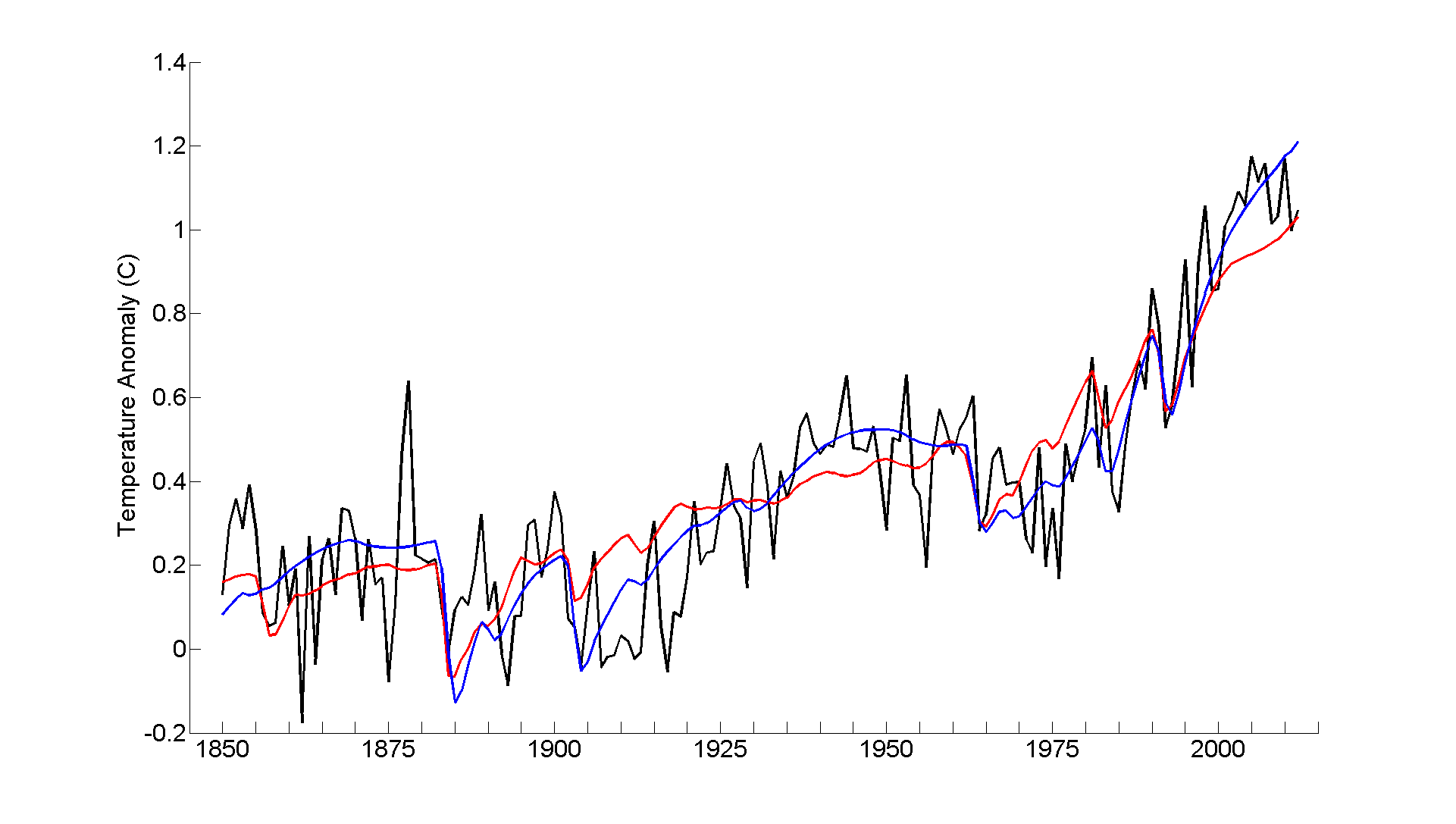 Fig 2. NH temperature anomalies from 1850–2012 per HadCRUT4 (black) and as simulated by Mann’s EBM (blue) and the alternative low sensitivity EBM (red)
Mann’s high sensitivity EBM and my alternative EBM
Mann’s EBM has an equilibrium/effective climate sensitivity (ECS) of 3.0°C and, unusually, no allowance for heat uptake by the ocean apart from in a 70 m deep mixed layer. As a result, its TCR – the simulated temperature rise from CO₂ concentrations doubling over 70 years as a result of 1% p.a. growth – is 2.8°C, very little lower than its ECS. His EBM uses a modest aerosol forcing that becomes only 0.3 W/m² more negative over 1950–1975. So why does its simulated temperature rise from 1920–1950, during the AMO’s upswing, but fall from 1950 to 1975, over which period the AMO was in a downswing but anthropogenic forcing excluding aerosols rose by over 0.7 W/m² (per AR5)?
The explanation is that Mann makes only a very modest allowance for the increase in non-CO₂ greenhouse gases and other non-aerosol anthropogenic forcings over 1950–1975, so his increase in total anthropogenic forcing over that period is only 0.4 W/m², 0.32 W/m² below AR5’s best estimate. During that period solar and volcanic forcings both had negative influences – totalling -0.2 W/m² per Mann’s data and -0.3 W/m² per AR5, taking trailing 5-year means to allow for the time constant of the ocean mixed layer. There was also sizeable negative volcanic forcing in 1963-64, again larger per AR5 than in Mann’s data. Therefore, Mann’s EBM had a negative forcing trend over 1950-1975 and shows cooling during that period.
On the other hand, during 1920–1950 the increasing trend in negative aerosol forcing was more than offset by trends in solar and volcanic forcings, and the very high TCR of Mann’s EBM made up for the shortfall in non-CO₂ greenhouse gas forcing and other non-aerosol anthropogenic forcings. After 1975, during the AMO upswing, much the same occurred, but by then the rise in CO₂ forcing was faster and more dominant, so Mann’s EBM simulated temperature rose fast. After 2000, since when the rise in CO₂ has strongly dominated changes in other forcings, Mann’s sensitive EBM outpaces HadCRUT4.
As a result of the particular forcing history used, Mann’s EBM, despite its very high TCR, is able to match – very closely on a smoothed basis – not only the overall HadCRUT4 20th century NH record but also its AMO-influenced ups and downs. But Mann chose the scaling for aerosol and solar forcing to optimise the fit, so it is not very surprising that it is good. The result is that his differenced-AMO smoothed time series is fairly flat over the 20th century, and declining post 2000.
My alternative, low-sensitivity, EBM is driven by the AR5 forcing best estimate time series. As is common when using a simple global model, volcanic forcing is scaled down, here by a factor of 0.5. It remains higher than the volcanic forcing series Mann uses for his EBM. The low-sensitivity EBM has the same ocean mixed layer depth as Mann’s EBM, but it is a 2-box model with the rest of the ocean’s heat capacity represented as well. The EBM has an ECS of only 1.65°C, in line with my best estimate using AR5 forcing and heat uptake data. One might expect a higher sensitivity (or a scaling of the simulated temperature) to be needed to match the warming in the NH, which is faster than the global rate, but different ocean parameters from those used for global temperature simulations suffice to allow for this.
The low-sensitivity EBM’s deep-ocean heat uptake coefficient is chosen to produce a TCR of 1.37°C which, on adding to the simulated temperatures a suitably scaled version of the 5-year mean NOAA AMO index, gives the best fit to the HadCRUT4 NH surface temperature record. That AMO index increases only modestly between the start and end of the simulation. The NH temperature simulated by my low-sensitivity EBM matches the overall NH temperature rise exhibited by Mann’s EBM up to the late 1990s, and matches the overall 1850–2012 observed (HadCRUT4) rise more closely. However, without the addition of the scaled 5-year mean NOAA AMO index the low-sensitivity EBM simulation’s fit to NH observations is a little worse than Mann’s in terms of mean square error, as it does not emulate the AMO’s fluctuations.
Mann’s differenced-AMO vs detrended-AMO
To recap, Mann’s differenced-AMO just represents actual minus model-simulated forced NH (not, as stated in the press release, North Atlantic) surface temperature. And whilst NOAA’s AMO Index is a detrended average of mean North Atlantic SST, for some unexplained reason Mann instead defines his detrended-AMO as the detrended average of mean NH temperature. In both cases, the AMO signal is smoothed by a 50-year low-pass optimising filter of Mann’s design – using slightly different variants in the two cases. Figure 3 shows the differenced-AMO (black) and the detrended-AMO (red), along with the unsmoothed annual time series that they are derived from.
Notice how Mann’s differenced-AMO, based on his EBM simulation, has a gentle peak just before 1990 before declining noticeably, so that it falls slightly from the mid-1970s to 2012. By contrast, Mann’s detrended-AMO rises strongly throughout that period. The smooth thick blue line shows the results of applying the detrended-AMO approach to the NH temperature evolution as simulated by Mann’s EBM. Its near coincidence with the smooth thick red actual detrended-AMO line shows how successful Mann has been in fitting his EBM to match the multidecadal fluctuations in NH surface temperature.
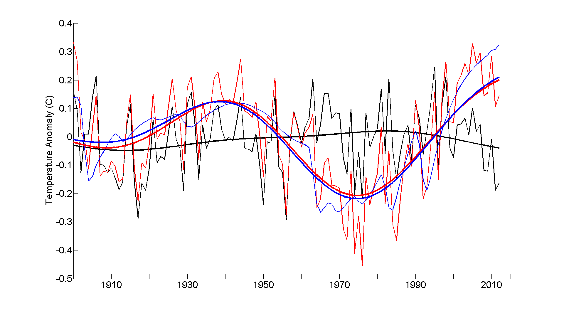 Fig 3. Version of Mann’s Figure 2.a). Estimated NH temperature anomaly variability: thin and thick lines are respectively annual, and 50-year low-passed smoothed, time series. The red lines show detrended observed (HadCRUT4) NH anomalies, the thick line being Mann’s detrended-AMO. The black lines show the observed NH temperature anomaly minus Mann’s EBM simulation, the thick line being the differenced-AMO. The blue lines show detrended anomalies from Mann’s EBM simulation, the thick line being what the detrended-AMO would be if based on the EBM-simulated rather than observed temperatures.
In Figure 2.a) of Mann’s actual paper (reproduced here as Figure 4), the smooth differenced-AMO line (grey dashed line in his figure) has a somewhat different shape, starting at a high level and ending at a lower level, with a peak around 1945 and minimum around 1965 that are missing when I run his code. The smooth blue line (in this case dashed rather than thickened) showing the results of applying the detrended-AMO approach to Mann’s EBM simulation is also marginally different. The EBM and smoothing code is deterministic so there should be no discrepancies.
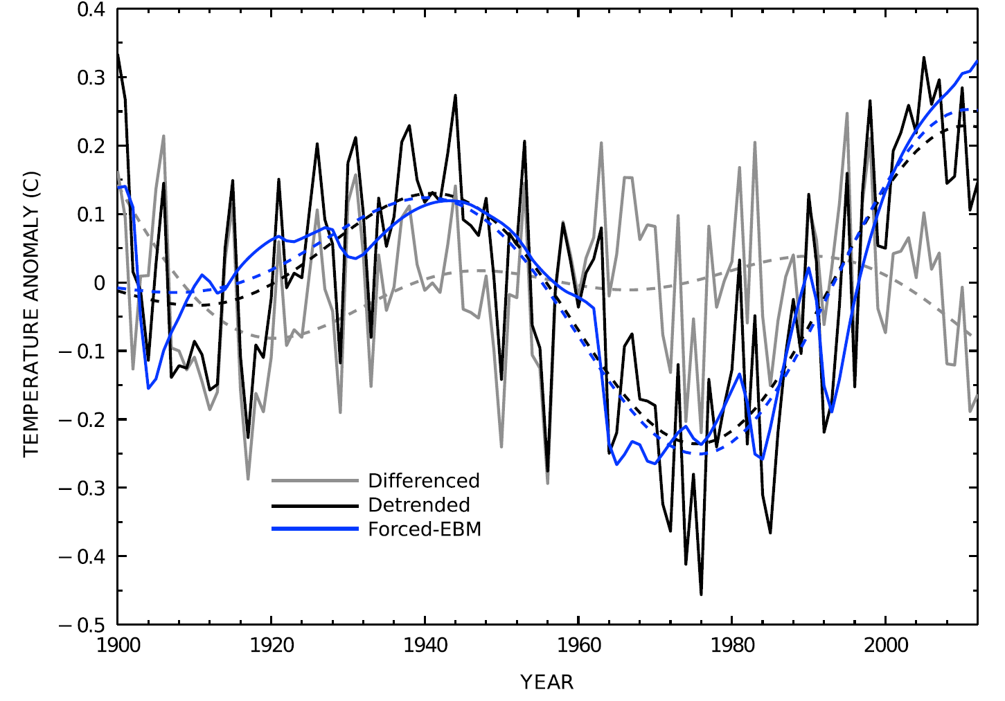 Fig 4. Reproduction of Figure 2.a) from Mann’s GRL paper. This shows the same time series as Figure 3 and should be identical to it, but with grey lines in place of black lines and black lines in place of red lines. Dashed rather than thick lines are used to show the smoothed AMO-like signal versions of the annual time series.
As the jagged blue lines (the detrended EBM simulation anomalies) do not differ visually between my and Mann’s paper’s version of his Figure 2a, it seems possible that the difference lies in the smoothing used. Figure 5 shows the effect of changing the cut-off frequency of Mann’s low-pass filtering from the “freq0=0.02; % low-freq cutoff in cycles/year” in his archived code to freq0=0.025. That changes it from 50-year to 40-year low-pass filtering, which is in line with what the code comment says:
% determine multidecadal compoments via 40 year lowpassed versions of the residual series
The results, shown in Figure 5, are indeed much closer to those shown in Mann’s paper, although not identical. However, with 40-year low-pass filtering Mann’s results, as reflected in his subsequent figures, differ noticeably from those in his paper (and are slightly less impressive). I will leave this mystery for the future and continue for the rest of my present investigation making use of the 50-year low-pass filtering specified in Mann’s paper (resetting freq0 to 0.02). That filtering has broadly similar effects, leaving aside endpoints, to smoothing by a 15 or 20 year moving average, but it suppresses shorter-term fluctuations much more strongly.
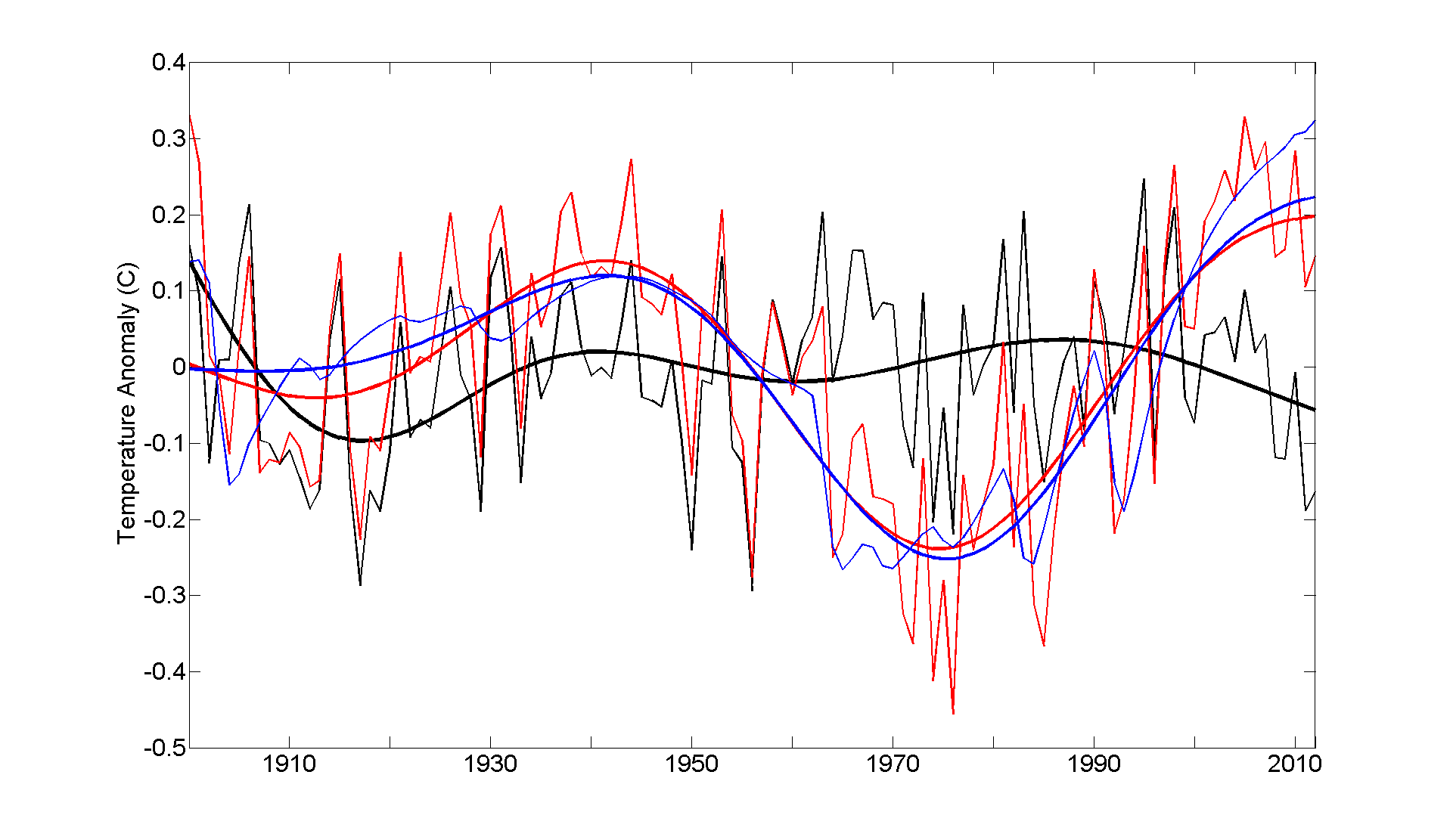 Fig 5. Same as Figure 3 but using 40-year rather than 50-year low-pass filtering
Mann’s case against the detrended-AMO
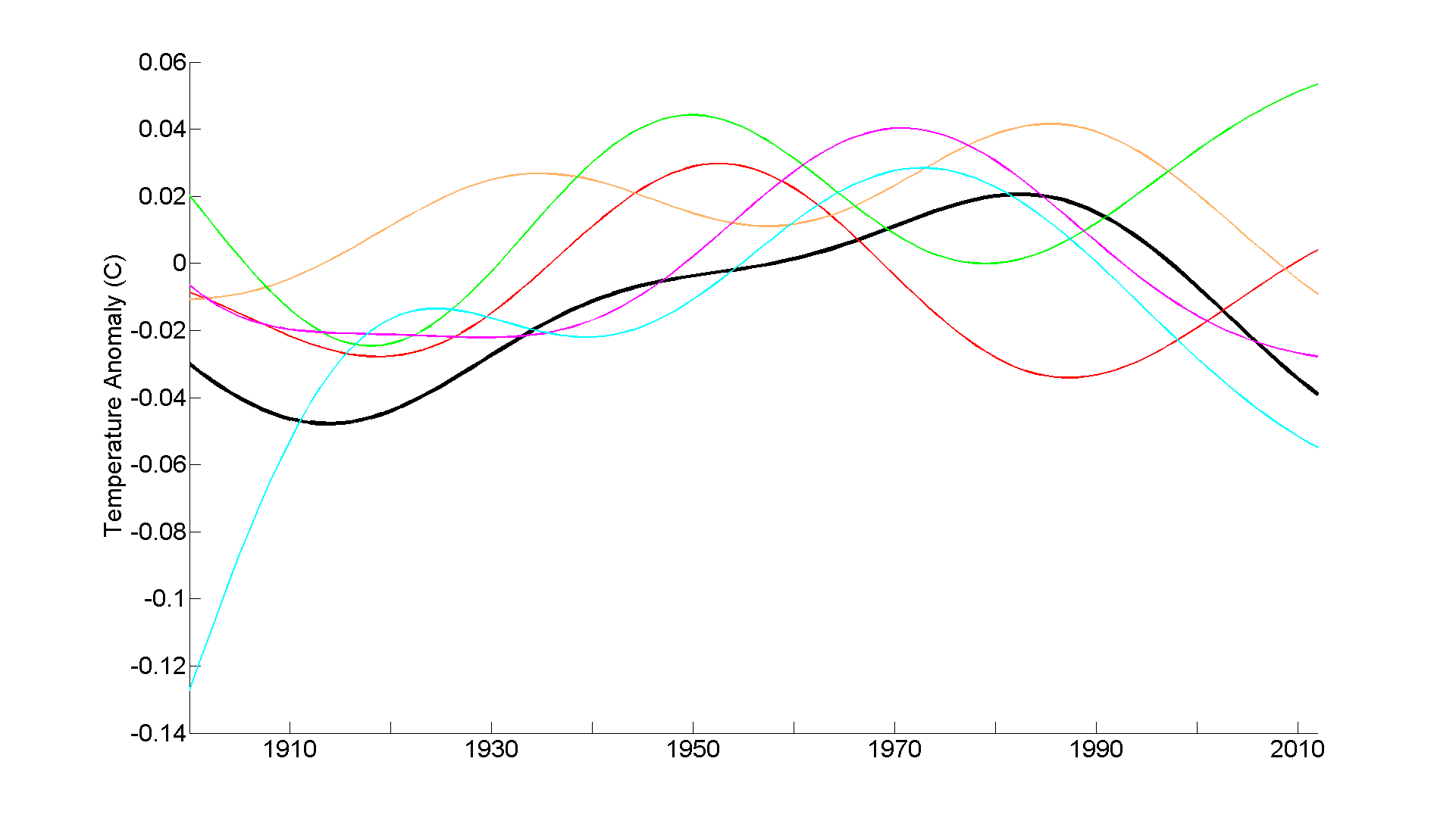
Mann’s key claim is that, where the signal is known a priori, the detrended-AMO approach to estimating AMO-related variability fails to isolate the true internal variability, and yields an excessive and out-of-phase estimate of the true AMO signal. His Figure 3a, a version of which based on running his code is reproduced as Figure 6a, shows the differenced-AMO signal from five noisy variants of his EBM-simulated temperature time series with random realisations of red noise added – the noisy series being treated as surrogate NH temperature observations – (coloured lines), and the differenced-AMO based on actual NH temperature observations (black line). In all cases the differenced-AMO calculation deducts the noise-free EBM-simulated temperature time series from the noisy series (leaving just the red noise) and then applies low-pass filtering. Mann points out that the differenced-AMO signals represent independent realisations of multidecadal noise and are therefore uncorrelated, with random relative phases and a small amplitude. That is obviously so.
Mann’s Figure 3.b), a version of which based on running his code is presented as Figure 6b, shows detrended-AMO signal estimates from the same five noisy EBM simulations (thin coloured lines) and based on observed temperatures (red line of Figure 3) (black).
Mann writes in his paper:
The random surrogates are qualitatively similar in their attributes to the differenced-AMO estimate of the real-world AMO series. By contrast, the detrended-AMO signals (Figure 3b [here 6b]) show amplitudes ~0.25°C that are inflated by more than a factor of two. Further, they are largely all in phase with the detrended-AMO signal diagnosed from observations (Figure 2 [here 3]), an artifact of the common forced signal masquerading as coherent low-frequency noise.
a)
 b)
b)
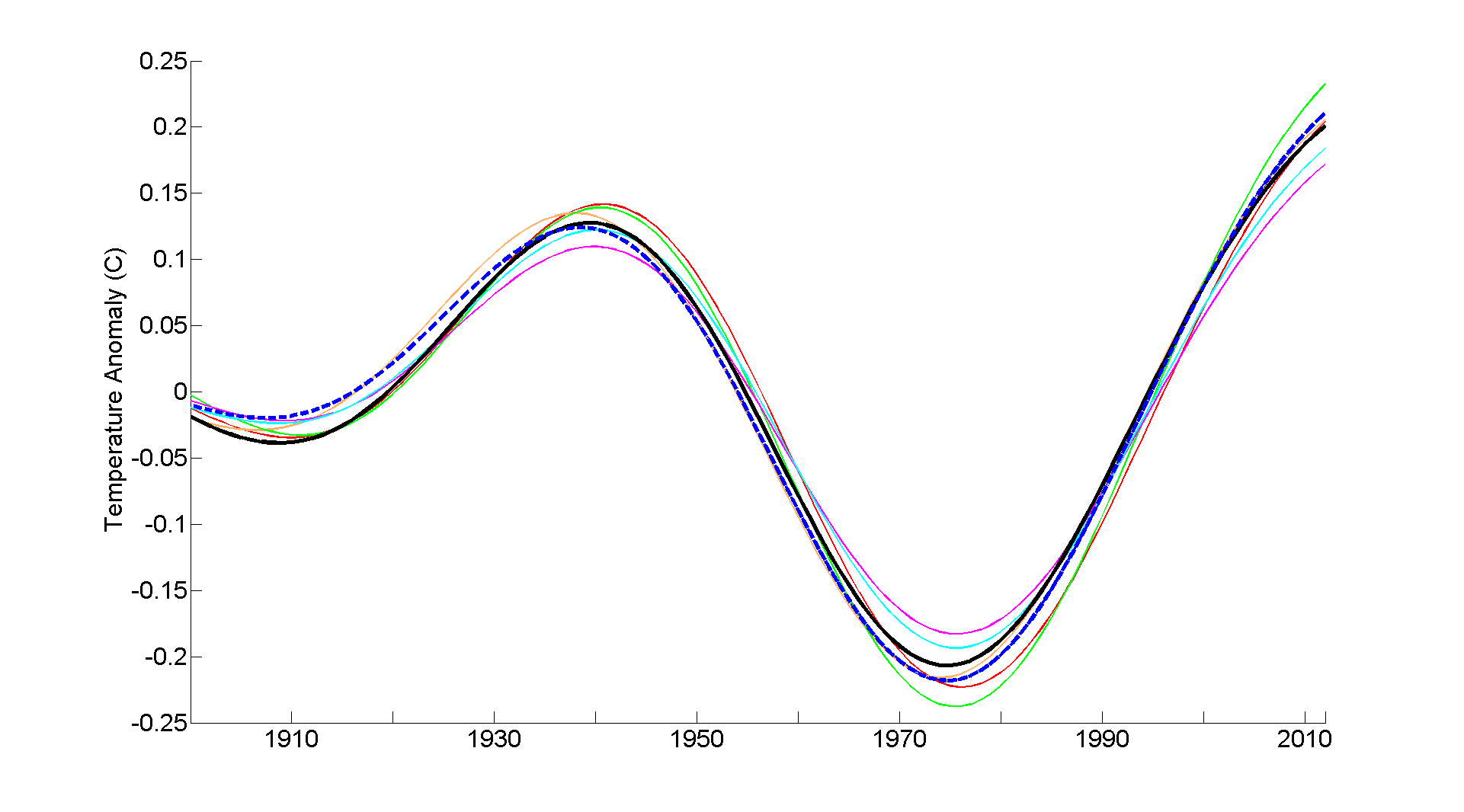 Fig 6. Version of Mann’s Figure 3. Comparison of (a) “true” pseudo-NH AMO signal (as a priori defined using the differenced-AMO approach, not the real AMO) and (b) NH AMO signal as estimated by detrended-AMO procedure, applied to surrogate observational time series consisting of five noisy variants of Mann’s EBM simulation. (a) The differenced-AMO signal estimates relative to the noise-free EBM simulation: from the noisy simulations (thin coloured lines) and from the actual observed NH temperature time series (black; same as Figure 3 black line, but different scale). (b) The detrended-AMO signal estimates: from the noisy simulations (thin coloured lines); based on observed temperatures (red line of Figure 3) (black); and from the noise-free EBM simulation (blue dashed; same as Figure 3 blue line: omitted in Mann’s Figure 3).
The flaws in Mann’s case
The first part of what Mann writes is obviously true, but are his conclusions warranted? It is true that the detrended-AMO signals diagnosed from the noisy EBM simulations are indeed largely all in phase with, and very similar in amplitude to, the detrended-AMO signal diagnosed from observations (the black line). But their real such relationship is to the detrended-AMO signal diagnosed from the noise-free EBM simulation. Although that signal is not shown in Mann’s published Figure 3b, it is actually plotted by his code, and is shown by the blue dashed line in Figure 6b (same as Figure 3 thick blue line). As can be seen both there and in Figure 3 above, the low-passed detrended-AMO signal diagnosed from observations and the low-passed detrended-AMO signal diagnosed from the noise-free EBM simulation are almost identical, reflecting the success of Mann’s fitting of his EBM simulation to the smoothed observations. Therefore, the detrended-AMO signals diagnosed from the noisy EBM simulations appear also to be related to the detrended-AMO signal diagnosed from observations. But that apparent relationship is purely an artefact of the similarity of the detrended-AMO signal diagnosed from observations and the detrended-AMO signal diagnosed from the noise-free EBM simulation.
Mann’s random red-noise series have low-passed components typically only a quarter as large as the smoothed signal from applying his detrended-AMO approach to the EBM forced simulation (compare coloured lines in Fig 6a with blue dashed line in Fig 6b, noting different scales). So it is unsurprising that one recovers something close to that signal (as in Fig 6b) – and hence close to the nearly identical detrended-AMO from observed temperatures (black line in Fig 6b) – when applying the detrended-AMO approach to the EBM forced simulation with the random red-noise added, whatever realisation of noise is used.
So Figure 6 does not prove Mann’s claim. The detrended-AMO signals are in reality largely all in phase with, and of similar amplitude to, the detrended-AMO signal diagnosed from the noise-free EBM simulation, not (as Mann claims) with that signal derived from observations. One would expect to end up with something close to a smoothed version of the signal when adding a noise component with a small low-frequency amplitude to a signal with a ~4 times larger low-frequency amplitude and low-pass smoothing their sum, where there are only two cycles of signal in the pass band.
Figure S7.b3 in Mann’s Supplementary Information, reproduced as Figure 7, very much supports my conclusion. It shows the results when an alternative volcanic forcing series (Crowley) is used. When that is done, the application of the detrended-AMO approach to Mann’s EBM simulation gives a significantly different signal (blue line – present, but not identified, in Mann’s SI graphs) from when it is applied to the actual temperature observations (black line), and the coloured lines cluster closely around the blue line rather than the black line.
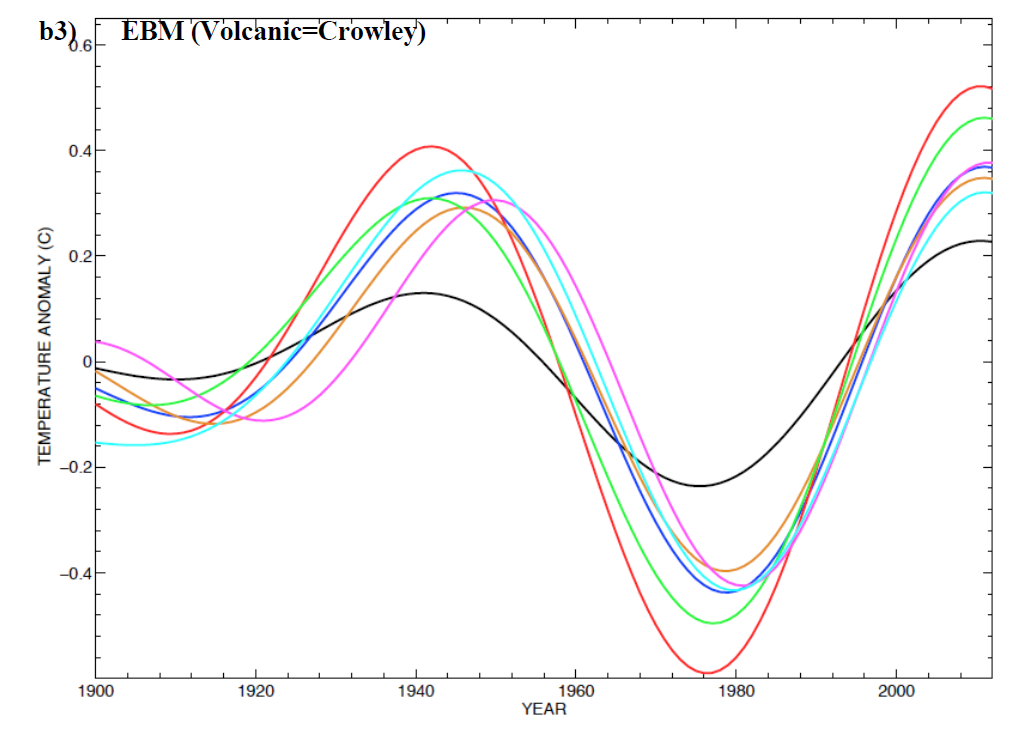 Fig 7. Reproduction of Mann’s Figure S7.b3: as Figure 3.b in his main article but using the Crowley volcanic forcing series. The detrended-AMO signal estimates: from the noisy EBM simulations (red, green, cyan, yellow and magenta lines); from observed temperatures (black line); and from the noise-free EBM simulation (blue line)
Mann’s attack on Stadium Waves
Essentially the same arguments apply to Mann’s critique of the “stadium wave” theory (Wyatt et al, 2012; Wyatt and Curry, 2013), about which the press release says:
Mann and his team also looked at supposed “stadium waves” suggested by some researchers to explain recent climate trends. The climate stadium wave supposedly occurs when the AMO and other related climate indicators synchronize, peaking and waning together. Mann and his team show that this apparent synchronicity is likely a statistical artefact of using the problematic detrended-AMO approach.
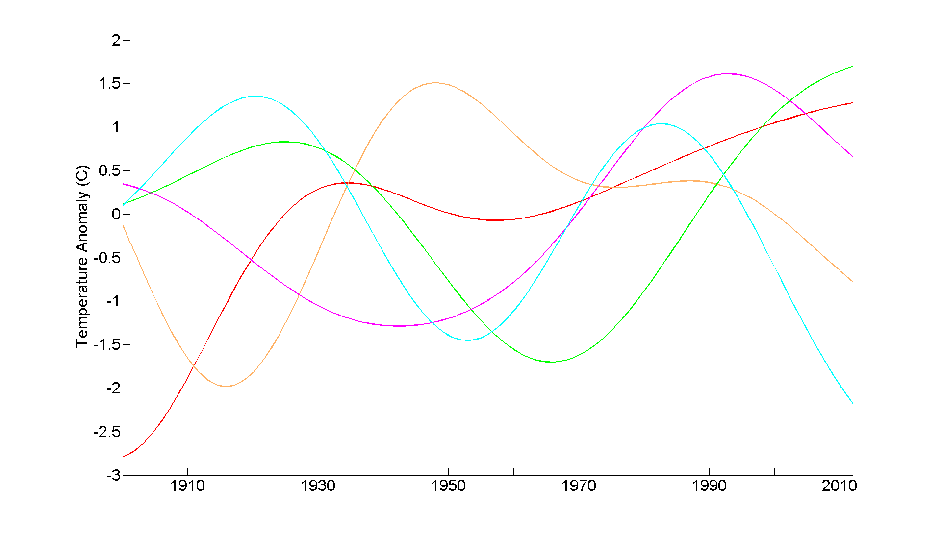
Mann applies a similar procedure to what he terms synthetic AMO-related indices, which are pretty well the same as the noisy EBM simulations used already but with noise of a larger amplitude added. Figure 8, a version of Figure 4 in Mann’s paper produced by running his code, shows the outcome. Mann writes in his paper:
Indeed, the detrended-AMO approach (Figure 4b [here 8b]) yields an apparent multidecadal AMO oscillation that is coherent across the indices, an artifact of the residual forced signal masquerading as an apparent low frequency oscillation. The apparent AMO signal is most coherent across indices during the most recent half century, when the forcing is largest. Another important feature apparent in this comparison is that the low-frequency noise leads to substantial perturbations in the overall “phase” of the apparent AMO signal (Figure 4b [here 8b]) giving the appearance of a propagating wave or stadium wave in the parlance of Wyatt et al. [2012].
However, the thick blue line in Figure 8b, plotted by Mann’s code but missing from his published figure, shows the AMO signal as estimated by Mann’s detrended-AMO procedure applied to the noise-free EBM simulation, gives the lie to this claim. Rather than being “an artifact of the residual forced signal masquerading as an apparent low frequency oscillation”, the thin coloured lines are seen as modified, phase-shifted versions of the signal from applying the detrended-AMO approach to the noise-free EBM simulation.
a)
 b)
b)
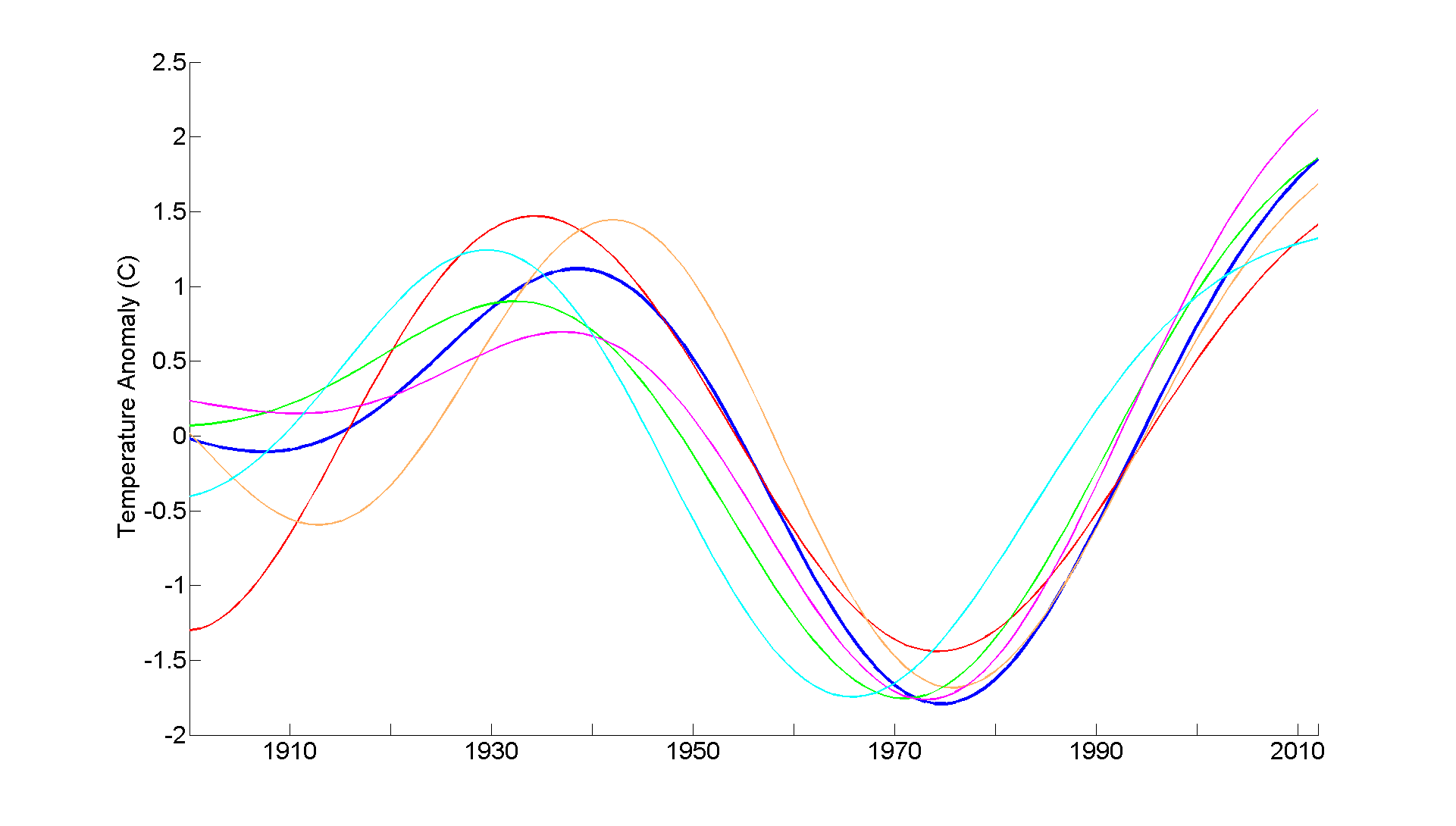 Fig 8. Version of Mann’s Figure 4. Comparison of (a) true pseudo-NH AMO signal (as a priori defined using the differenced-AMO approach) and (b) NH AMO signal as estimated by detrended-AMO procedure. In both cases, no actual observational data is used: results are shown for the five synthetic standardized climate indices as described in Mann’s text, derived using his EBM simulation with added noise realisations (thin coloured lines). In (b) the result of applying the detrended-AMO approach to the noise-free EBM simulation is also shown (thick blue line; scaled version of that in Figure 3: omitted in Mann’s Figure 4). Series are standardized to have unit variance.
The results shown in Figure 8b are what one would expect to arise: a noise amplitude that is greater relative to the signal than before causes more modification and phase-shifting of the clean signal: (compare Figure 8b with Figure 6b). The extent of the differences between the coloured lines in Figure 8b derived from the noisy synthetic AMO-related indices and the blue line derived from the noise-free EBM simulation varies with the random realisations of noise, and can be much greater. The corresponding graphs (Figures S8.b9 and S8.b10) based on the GISS-E2-R and CMIP5 Ensemble simulations show a gradual loss of coherency between the five noisy versions and the detrended-AMO based on the forced simulations (the blue lines, which do appear in the graphs in Mann’s Supplementary Information). Before ~1960, the GISS-E2-R and CMIP5 Ensemble simulations do not follow the real-world detrended-AMO signal as well as Mann’s EBM simulation does.
Results using the low-sensitivity EBM
So far, I’ve been repeating Mann’s analysis using his EBM simulation. Now I’ll look at what happens when my low-sensitivity EBM simulation is used instead. Figure 9 shows the same as Figure 3 (my version of Mann’s Figure 2a) save for my low-sensitivity EBM simulation being used instead of Mann’s EBM simulation. Unlike the situation with Mann’s EBM simulation, the thick blue line (detrended-AMO based on EBM simulation) is not almost identical to the thick red observational detrended-AMO line, and the thick black line – the differenced-AMO – does bear a resemblance to the observational detrended-AMO.
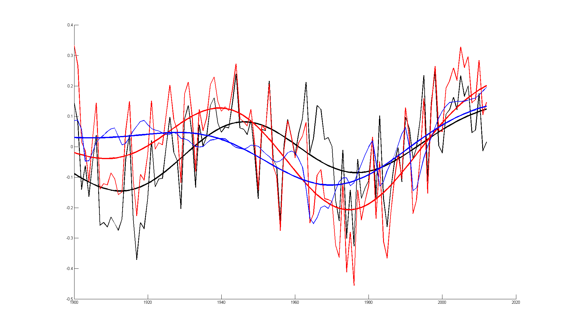
Fig 9. Estimated NH temperature anomaly variability 1900-2012: thin and thick lines are respectively annual, and 50-year low-passed smoothed, time series. The red lines show detrended observed (HadCRUT4) NH anomalies, the thick line being the detrended-AMO. The black lines show the observed NH temperature anomaly minus the low-sensitivity EBM simulated temperature, the thick line being the differenced-AMO. The blue lines show detrended anomalies from the low-sensitivity EBM simulation, the thick line being what the detrended-AMO would be if based on the EBM-simulated rather than observed temperatures.
Figure 10 shows the same as Figure 6b (Mann’s Figure 3b) but using the low-sensitivity EBM simulation instead of that from his EBM. It is now fairly obvious visually that the coloured lines resemble the blue dashed line that represents an application of the detrended-AMO approach to the EBM-simulated temperatures, rather than resembling the black line representing the detrended-AMO derived from observed NH temperatures. That is confirmatory evidence that my analysis of what is going on is correct.
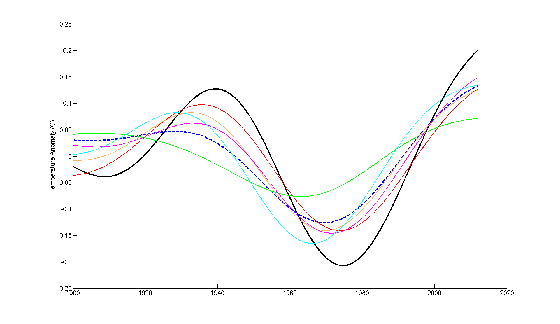 Fig 10. Version of Figure 6.b) based on the low-sensitivity EBM simulation
Is the detrended-AMO nevertheless questionable?
The detrended-AMO approach is not perfect, even when applied – as is standard – to SST temperatures in the North Atlantic, not to the full NH land and ocean surface temperature as Mann does. When the rate of increase in forcing secularly increases, as it has over the last hundred years, it is possible that the detrended-AMO may be biased towards high strengthening in recent decades. A comparison of the post mid-1970s segments of the red line (detrended-AMO from observations) and the black line (differenced-AMO from low-sensitivity EBM simulation) in Figure 9 illustrates this point. However, the basic shapes of the two lines are similar, and the differenced-AMO still accounts for about a 0.2°C rise in NH temperature over the last thirty or so years.
It would be preferable to find a way of estimating the AMO that was more independent of forced temperature trends. That is, in effect, what Delsole et al (2011) did in estimating their internal multidecadal pattern (IMP) in global SST. They employed a sophisticated statistical method based on maximising average predictability time, using simulations by a number of CMIP3 coupled GCMs as well as observed SST, to separate forced and unforced variability in SST. Although their method applies globally, the IMP they detect is remarkably similar to the standard NOAA detrended-AMO index. Figure 11, a reproduction of Figure 4 from Delsole et al’s paper, compares NOAA’s AMO index, suitably rescaled, (red line) with the ±1 standard deviation uncertainty range of their estimated IMP (shaded grey). The fit is remarkably close.
Using a different sophisticated statistical approach, Swanson et al (2009) also found an AMO-like pattern of multidecadal unforced variability, here in GMST rather than global SST, although with a somewhat lower recent level.
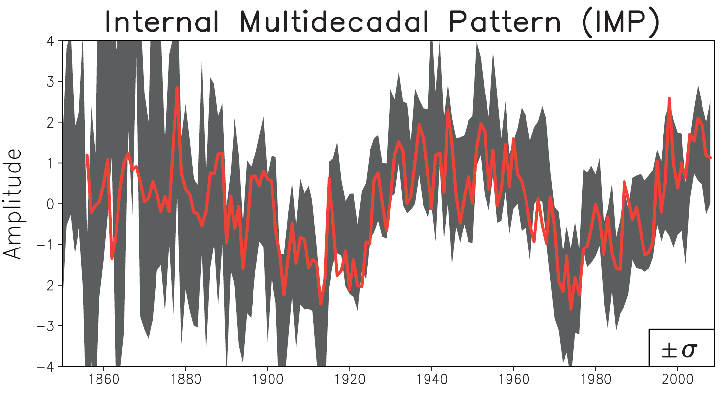 Fig. 11. Reproduction of Figure 4 from Delsole et al (2011). ±1 standard deviation uncertainty range of their estimated IMP (shaded grey) and scaled AMO index from NOAA based on detrended North Atlantic SST (red line). The vertical scale is arbitrary.
Finding a physical explanation for the AMO is of course desirable, and likely to lead to better estimation of its influence on temperatures and other climate phenomena both globally and regionally. That is a major attraction of the stadium wave theory. If it holds up under further examination, it promises a better understanding and estimation of multidecadal internal climate variability. Other papers, such as Dima & Lohmann (2007), have also put forward possible natural physical mechanisms for the AMO.
Conclusions
I have shown that the evidence Mann claims disproves the detrended-AMO, and supports his differenced-AMO, is illusory. I have also shown that his code produces different results from those shown in his accepted paper. I have pointed out that graph lines produced by his code that would have made it much easier to spot the flaws in Mann’s evidence, although appearing in the figures in his Supplementary Information, were omitted from the figures in his main paper.
A differenced-AMO approach has attractions in principle, but only makes sense if climate models are near-perfect, which is far from the case. The ease with which a simple EBM model can have its parameters adjusted to produce a nearly flat differenced-AMO shows the very low number of degrees of freedom involved, with only two full AMO cycles during the instrumental period. The very heavy, 50-year low-pass, smoothing applied by Mann arguably exacerbates this problem.
The detrended-AMO approach is not perfect, but the pattern exhibited by NOAA’s standard detrended AMO index based on North Atlantic SST appears to be supported by much more sophisticated approaches. The stadium wave theory, if it holds up, offers physical insight into the mechanisms underlying the AMO and may lead to more reliable estimation of its state and influence on surface temperatures and other climate variables.
Nicholas Lewis
A pdf version of this article is available here.
[i] Enfield, D.B., A.M. Mestas-Nunez, and P.J. Trimble, 2001: The Atlantic Multidecadal Oscillation and its relationship to rainfall and river flows in the continental U.S., Geophys. Res. Lett., 28: 2077-2080


62 Comments
Nic. Compliments Re: Mann “defining the AMO as the part of the smoothed temperature change simulated by the models that is not observed”. Mann complements the UNFCC’s redefinition:
‘Mann’s case is built on results that do not support his contentions’
Least surprising news in the world?
…
Mann misrepresents himself.
I do hope you send in a letter to the Journal summarising this.
Good work.
One of the points that I take from this comment/essay is that proper “peer review” is time consuming, requires significant effort and expertise and is in no way trivial.
It simply highlights the difficult in creating a well organized meaningful and significant — yet error free paper without feed back of someone willing to challenge your every position.
I am in no way excusing the authors of the original paper.
Fascinating and very well communicated post. Mann is a formidable fellow. By simply assuming that the models are basically correct, he gives himself all sorts of possibilities for statistical manipulations, and in the process manages to turn both the AMO and stadium wave hypothesis sideways so that he can skewer them both with the same stick!
I remember a highly criticised paper by a McIntyre and McKitrick showing some methodology flaws in certain temperature reconstructions by pointing out that no matter what you put in — out pops a HS signal through a noisy beginning and an instrument data ending… And yet here, is not Mann turning our knowledge of the AMO fully on its head claiming it as an artifact because it can appear through noise no matter what you put into his AMO methodology? Am I off on detecting similarities? If not, such ironic lengths to defend the correctness of models.
So GIGO has become GIAMOO?
Prof. Mann doing math to arrive at a politically correct conclusion… What could possibly go wrong? Was there also a counter-intuitive inverse AMO signal in the Graybill bristlecone pine strip-bark series or the Tijander sediments? Stayed tuned!
I also love the methodological starting point of seeing reality as an exception to the models that needs to be explained away or recast as confirmation.
As a technical matter, I wonder whether Prof. Mann has stepped outside the scientific consensus regarding the AMO (it would seem so!). Or does the consensus go wherever Prof. Mann goes by defiinition?
Does Mann argument goes like this? while adding noise, the detrending algorithm shows itself to beunreliable, because it shows similar results.
And you, Lewis, are saying the conclusion don’t follow because the noise is too small?
Stand back Nic.
You have unleashed the beast…
Interesting deconstruction of Mann’s work, even if I only understood parts of it.
I do have a minor gripe though. It would be nice if a continuation-break could be inserted after a few paragraphs at convenient location. There are now a couple pieces on the main page which are making make it somewhat unwieldy to navigate.
Ahhh. I thank you, and I’m sure those laboring under bandwidth caps also appreciate the main page modification.
That I grok. Presumably nothing can be deduced about TCR as a result of these statistical shenanigans. How many years of instrumental records are going to be needed before we can begin to speak with confidence of phenomena like the AMO?
It reads as a brilliant investigation and explanation, Nic, of which readers like myself will understand just a little. Also handy background to the Stadium Wave theory. One wonders what the original author will say in response. He managed not to mention The Hockey Stick Illusion in his book on the subject but you’re much closer to researchers in related areas and I assume he’ll find it harder to blank you. The sociology should be gripping if nothing else.
The premise of the study is to show that the present 15-17 year cooling/non warming is due to the AMO and that the excessive warming of the late 1970’s through 1998 was only partly due to AMO. Though I find it implausible to cooling trend of the AMO is more prominent that the warming trend – should the warming/cooling trends of the cycle be roughly the same.
The second point with respect to the models – If these climate scientists are so much smarter than us mere mortals, then why did they not factor the AMO into the climate models.
Several months ago, I attempted to follow/trace the AMO & PDO oscillations back though the beginning of the hockey stick to see if it followed the 60-70 year cycle. My methodology was unfortunately crude.
Has anyone had better success on determining if the hockey stick graph followed or did not follow the cycle?
Steve – If you have had a chance to look into this issue, can you please comment, Thanks
When this paper was initially brought up at SKS I made the following comment that is appropriate here for this thread:
“Although the stadium wave is undoubtedly an incorrect hypothesis – I consider the counterintuitive result of the recent Mann et al (2014) study to require greater scrutiny. In particular this result does not
The issues with the method are related to the input parameters of the energy balance model he uses, the accuracy of the forced components used and finally the lack of any spatial figures. IF this method is appropriate then he should be showing a spatial amplitude map and it should have the same spatial pattern as would be expected based on theory behind the mechanisms. This is somewhat a glaring omission. I think he provides a compelling case that the detrended AMO is inappropriate but I think his solution is theoretically appropriate but in practice is not sufficiently justified based on the paper. I also did not like that he cited Booth and other aerosol forcing AMO studies without citing their rebuttals which were compelling (e.g. Zhang et al. 2014). The argument that the AMO was positive during the 1990s and is negative currently is at odds with the spatial distribution of temperature changes over that period – particularly in the Labrador Sea. In this area the temperatures are warming faster than projected by GCMs and were faster during the mid-century and cooler during the 1970-1995 section. This temperature history for one of the main nodes of the “amo” is at odds with the history implied by Mann’s version. I suspect many of the experts on the physical mechanisms behind the AMO will disagree strongly with his new reconstruction of this index.
I think any “new definition” of an AMO needs to be supported by more than just time series analysis – there needs to be a physical understanding of the underlying mechanism. A point made in Climate Dynamics last year. Did they check to make sure these results made sense with respect to the underlying mechanism? Did they relate it to salinity and sea ice ? As a mode of NH temp variation it is possible there is some relation to this index – however the AMO which is traditionally referred to by authors was not cooling over the past 15 years.”
Some of the concerns I listed above pertain to the analysis presented here as well – there is in effect a wealth of literature which is on the subject that examines the pros and cons of different approaches and the physical mechanisms underlying each. The aerosol theory as being the driver of the AMO is not justified in my view but likewise it is an important consideration – particularly given that many of these additional forcings are prominent in the North Atlantic. Tom Crowley’s (Rest in Peace) recent paper does provide some interesting results as well: http://onlinelibrary.wiley.com/doi/10.1002/2013EF000216/pdf
So what ends up constituting a submission that is worth rejection because it is at odds with prevailing climate science vs. acceptance because of the potential to be of high impact if confirmed?
It appears in recent times we have good examples in which papers that ‘shake things up’ were given the peer-reviewed light of day despite their controversial-ness/misgivings, whilst others were not.
Here, Nic would have argued for rejection of this paper, though presumably would have green-lighted Begnsston’s paper. Others have obviously come to an alternate conclusion.
Robert
Thanks for your useful comment. As you say, the rebuttal of the Booth et al aerosol forcing study by Zhang et al was compelling. And I also had found the recent Crowley paper’s results interesting.
As I wrote in my article, I in fact agree that simply detrending the NA SST series may well not be appropriate when forcing has been increasing (at least when that has been at a varying rate). However, why do you claim about Mann’s paper:
“I think he provides a compelling case that the detrended AMO is inappropriate”.
Would you not agree, having read my article, that the case Mann provides that the detrended AMO is inappropriate is in fact just smoke & mirrors – there is no real case there at all? If not, may I ask why not?
Ill take a moment to comment when I get a chance – but here is a paper relevant to the discussion
Click to access art%253A10.1007%252Fs00382-014-2176-7.pdf
Combined influences of seasonal East Atlantic Pattern and North
Atlantic Oscillation to excite Atlantic multidecadal variability
in a climate model
The mechanism discussed in the paper doesn’t make sense with the *new* AMO definition proposed by Mann et al 2014. Especially when you look at the salinity and NAO data over the past 4 decades.
Dr. Way,
If you are still around, a brief description of the evidence that the stadium wave hypothesis is “undoubtedly incorrect” would be greatly appreciated.
Steve: keep in mind that flaws in Mann’s criticism does not imply that the hypothesis is thereby “correct”.
To clarify, I did read Mann’s criticism of the stadium wave. He used the term “likely” wrong, and you here stated that time series analysis alone is not sufficient to create a new definition of the AMO. Combining this with your description of the stadium wave as “undoubtedly incorrect,” it seems you must have other lines of evidence that conflict with the stadium wave hypothesis.
Has Tom Cowley died? I had a very amiable exchange of emails with him once. He was a very nice man.
geronimo see – http://www.theguardian.com/environment/climate-consensus-97-per-cent/2014/may/15/passing-of-climate-giant-tom-crowley
Nic:
Hah! You didn’t think that he would provide a turn-key code producing all the figures etc., did you? 🙂 Actually this is the best I’ve seen from our Mann, the code actually runs, there are no missing files and no error messages are produced!
These small Mannian mysteries are nice to solve … you feel like Sherlock Holmes. Usually these mysteries are nothing important,but sometimes although you may not solve the actual mystery, the mystery leads you to other more important things. I think it may be also the case here …
Look how Mann is performing his smoothings. In the code he’s using the function “lowpassadaptive”. That’s simply his infamous “standard” (Mann08) smoothing method, in which the “best boundary condition” (endpoint filtering) is chosen from three possible candidates (min slope/norm/roughness). But this time he has also introduced another method “lowpassadaptive2”, which is exactly as the original but the “best” is chosen only from slope/norm candidates, i.e. Mann’s favorite “roughness” criterion is missing! Why on Earth you need to introduce that?!? Shouldn’t the same smoothing method be applied to all series? The short explenation about this in SI makes no sense whatsoever. BTW, it is easy to see in the code which series are smoothed with original method and which with the new: all the series with “good” in the variable name are smoothed with “lowpassadaptive” (the original) and all the series with “bad” in the variable name are smoothed with “lowpassadaptive2” (i.e., without “roughness” option). I’d guess smoothing the “bad” ones with the original method has some undesirable effects to the figures…
Clearly, “lowpassadaptive2” makes the “bad” series smooth properly.
Bad boys bad boys, whatcha gonna do? Whatcha gonna do when it’s lowpassadaptive2?
Jean
I too was impressed that the code and data were complete and ran!
Yes, I also saw which smoothing method was used for which type of series. Suspicious, as you say. But as I could show that whathe was doing was all smoke and mirrors without changing his smoothing methods, I didn’t attempt to do so – apart from trying out higher cut-off frequencies to see if I could reproduce the figures in his paper. Maybe if I had altered the smoothing type as well I would have succeeded in doing so.
“lowpassiveadaptive”. Hmmm. It has a certain resonance, does it not? It sounds like a term Stephan Lewandowsky might use to describe Michael Mann’s state of mind – or his own for that matter.
I like it very much. I think it should be more widely used. The Low Passive Adaptive Theory of Global Warming has a lovely ring to it. “Its very LPA, is it not?” rolls off the tongue. Funding has been secured for 10 years research into Low Passive Adaptive methodologies.
Why do they call it a “Stadium Wave” theory? Isn’t what they are describing like a Beat freaquency?
It is very much like a beat frequency or subharmonic. It’s sub-optimal to come up with a new term for an existing phenomenon, especially one that’s so well-understood in fields like electronics, acoustics and signal processing.
Unlike a beat frequency, this one propagates around the northern hemisphere like the sports stadium wave. Hence the name. Judith or Marcia would be glad to explain further, as they are both very accessible.
Michael Mann “recharacterizing” things, Steve. You are way, way, way to diplomatic methinks. It seems to me that Michael Mann digests raw information, feeds his ego and produces crap.
I guess I finally understood what Mann did. I hope I’m correct.
Using slightly “unorthodox” forcing, Michael Mann manages to get a good fit for multidecadal fluctuations in NH surface teperature.
Then he compares the detrended-NH method (which isn’t really AMO, but fine) applied to observed temperatures and modelled temperatures. (because of the good fit mentioned before, the results are quite similar). He also plot his difference-NH method. Mann’s AMO is of small magnitute, slightly cooling after the late 90s.
To show the detrended-NH method is incorrect, he creates some noisy models, and applies both methods to the model outputs. Small noise. Not surprisingly the “true” difference-NH method gives somewhat different AMO’s[1], all of small magnitude, and all the signals from the detrended-NH method gives very similar AMO’s (after all, the noise is small). Michael Mann claims this is an artifact, but, honestly, I didn’t understand his explanation. I guess one shouldn’t use a method that is too unsensitive.
The Supplementary Information shows that different forcing changes the model results (not really that surprising). As he is applying the methods to model results, the “AMOs” change too. Failure to model temperature oscillations.
Then he criticizes the stadium-wave hypothesis. For that, his plot shows that when you apply large noise, differenced-NH method shows different results[1]. The detrended-NH method shows somewhat different AMO’s for each noisy model (the technical words for that: phase-shifted and modulated), unlike what Mann’s said (that they are similar apparent oscillations, due to some artifact)
[1] the differenced-AMO from noisy models aren’t much different from smoothed red noise.
I didn’t attempt at being precise, as my idea was to formulate a less-technical string of thought.
I believe that the AMO signal, its fingerprint, is present in salinity data and in the distribution of ocean temperature anomalies, not just in overall temperature anomaly. Mann needs to address those as well.
an aside, while Michael Mann has claimed priority for coining the name “AMO” this claim is contradicted by several sources/considerations:
[h/t DCA at Climate, Etc.]
I got only as far as “Mann’s EBM has an equilibrium/effective climate sensitivity (ECS) of 3.0°C and, unusually, no allowance for heat uptake by the ocean apart from in a 70 m deep mixed layer. As a result, its TCR – the simulated temperature rise from CO₂ concentrations doubling over 70 years as a result of 1% p.a. growth – is 2.8°C.”
I gather that others have understood this, so I would appreciate an explanation for those of us who struggle with this stuff. I do understand that 3.0°C is considered a high sensitivity, but where does it come from in that “one-box” model? An ECS / TCR ratio of 3.0/2.8 sounds like a relatively short time constant, so I wouldn’t have thought the time constant is the source of the sensitivity. But I wouldn’t have thought that the pre-feedback “forcing” due to CO2 concentration is controversial, either.
Specifically, Mr. Lewis appears to contend that Mann’s energy-balance model is simply a “one-box” model, which I’ve been given to understand means a first-order differential equation, i.e., dy/dt = ax – by, where y is the temperature anomaly, x is the difference between CO2-caused “forcing” and its pre-industrial level, a is the reciprocal of the effective-depth-heat-capacity product, and b is the ratio of the negative algebraic sum of feedbacks to that product; i.e., b is the reciprocal of the system time constant.
Given that everyone seems to accept that forcing is logarithmic with CO2 concentration, the defined 1%/year exponential increase in concentration suggests a linear increase in forcing, so x = rt, where t is time and r is a positive real constant. That is, dy/dt = art – by, which implies that y = (ar/b)[t – (1/b)(1-exp(-bt)] if I’ve gotten my sums right.
In other words, transient climate sensitivity is (70 ar/b){1 – [1/(70 b)](1-exp(-70 b)}, and equilibrium climate sensitivity is 70 ar/b. If I’ve again gotten my sums right, that implies only a modest time constant: 1/b < 35 years, which isn't something I had previously understood to mean high sensitivity. That leaves ar, i.e., the ratio of CO2-forcing increase to heat capacity as the bad actor, but I hadn't previously thought those quantities controversial.
Since Mr. Lewis disagrees with Dr. Mann's sensitivity assumption, I would have assumed that Mr. Lewis disputes one of these parameters, but, for the reasons I've just given, I don't see which one. Obviously, I've made an invalid assumption somewhere along the way, and I'd appreciate it if someone could point it out.
Joe
I’m not sure I’ve quite followed your figuring, but I can confirm that Mann’s one-box EBM has a fairly short time constant, about 4 years. The effective-depth-heat-capacity product is 70 m * 71% ocean fraction * 4.1e6 J/m^3 K = 2.0e8 J/m^2 K. The negative feedback is the ratio of the forcing from doubled CO2 to the ECS, or 3.7/3.0 = 1.2 W/m^2 K. The ratio of these two factors is 1.6e8 seconds, or about 5 years.
Normal climate models do not have a single time constant, and those with an ECS of 3 K typically have a higher first time constant than 5 years and a much slower overall response. But there is nothing to prevent a model with an ECS of 3 K having a short time constant, although that results in an unrealistically high TCR.
I’ve just got a minute, so I’m going to argue past you and then circle back later to digest your response above, for which I thank you.
By my reckoning–which is only occasionally accurate–an ECS / TCR ratio of 3.0 / 2.8 means a time constant of 34.8 years: if a ramp in stimulus stops increasing at 70 years but the response continues to rise from its 70-year value of 2.8 asymptotically to 3.0, that’s what I calculated: 34.8. But I’ll go back and look at your numbers when a time slot opens up.
Thanks again.
Mr. Lewis:
I see now that my original question was based on a misapprehension about what qualifies as a “low” time-constant value in this context. So the ultimate answer to my original question is that, although you are using a “two-box” model yourself, you would in the context of a one-box model disagree with using as low a magnitude of negative feedback–and thus as high a time constant–as Dr. Mann used.
Specifically, if we use a “one-box” model and agree on the heat capacity and linearly increasing forcing, then it is true, as I implied, that the assumed feedback dictates time constant as well as ECS and TCR: if you have a lower time constant, ECS and TCR will be lower, and the ratio of ECS to TCR will, too, as can be seen in the equations the code below embodies. However I had been thinking of a “low” time constant as low in comparison with values I had heard in what must have been the results of higher-order models, where those simple relationships do not prevail. In the context of “one-box” models, five years is actually a high time-constant value.
I also see that my conclusion that the quoted ratio of ECS to TCR implies a 35-year time constant was the result of an error in copying my hand-written equation into code: I left the “1 -” out of my previous version of ECSoverTCR() below. With that correction, the numbers you gave me above are consistent with the 5-year time constant you quote.
Running the code below demonstrates this and plots the one-box model’s response to the assumed CO2-caused stimulus. The money result is given by the penultimate code swatch, in which ECSoverTCR(b) is shown to approximate 3.0 / 2.8, i.e., the ratio of Dr. Mann’s ECS to his TCR.
####################################################################################
# Single-Pole-System Simulation: dy/dt = ax – by
# Response to stimulus that increases linearly at rate r from value 0 at time 0:
yRamp = function(a, b, r, t, y0 = 0) y0 * exp(-b * t) + a * r / b * (t – 1 / b * (1 – exp(-b * t)));
# Response to stimulus = 0 for t 0:
yStep = function(a, b, x_ss, t, y0 = 0) y0 * exp(-b * t) + a * x_ss / b * (1 – exp(-b * t));
# ECS/TCR: For a given decay rate b, assume a stimulus that rises linearly over
# 70 years to a plateau that extends to infinity, and find the ratio of the
# response at infinity to the response at 70 years:
year = 365.2425 * 24 * 3600;
ECSoverTCR = function(b, T = 70 * year) T / (T – 1 / b * (1 – exp(-b * T)))
# From Nic Lewis:
x_ss = 3.7; # Steady-state “forcing,” in W/m^2
y_ss = 3.0; # “ECS”: steady=state response
a = 1 / (2e8); #reciprocal of product of effective depth and heat capacity
# Exponential CO2-concentration increase -> linear “forcing” increase, so:
r = x_ss / (70 * year); # Rate of CO2-caused forcing increase
# At equilibrium dy/dt = 0 -> ax_ss = by_ss, so:
b = a * x_ss / y_ss; # Reciprocal of time system time constant
1 / b / year; # Time constant: 5.138714 years
# Confirm that b (= reciprocal of time constant) results in the correct ratio of
# ECS to TCR
ECSoverTCR(b) # 1.079226
3 / 2.8; # Ratio of ECS = 3 to TCR = 2.8: 1.071429;
# Plot the response to the assumed ramp-to-plateau stimulus, assuming quiescence
# at t = 0:
N = 150;
t = year * 0:N;
y = yRamp(a, b, r, t[1:71]);
y = c(y, yStep(a, b, x_ss, t[72:(N + 1)] – 70 * year, y[71]));
plot(t / year, y, type = “l”, xlab = “Years”, ylab = “Temp. Anomaly”);
abline(v = 70, h = c(y[which(t / year == 70)], 3), lty = 3);
title(main = paste(“Response to 70-year ramp; time constant =”, round(1 / b / year, 2)));
######################################################################################
Thanks again for the response.
Just for fun I tried to derive the equation. What I came up with was:
(1/70 * tau)(-exp(-70/tau) + 1)=(ecs-tcr)/ecs
With (ecs-tcr)/ecs = .2/3 = 1/15
So plugging this into Wolfram alpha I get tau~4.66667 which I think is right.
http://www.wolframalpha.com/input/?i=%281%2F70+*+tau%29%28-exp%28-70%2Ftau%29+%2B+1%29%3D1%2F15
AJ:
Your expression for (ECS – TCR) / ECS is consistent with the derivation I used for the R functions in my comment above, where yRamp() evaluated at 70 years gives TCR and yStep() evaluated at infinity gives ECS, but plugging in Mr. Lewis’s numbers (3.7, 3.0, and 2e8), as I did, results in a TCR of 2.78 rather than 2.8, which I believe is why I got a time-constant value of 5.14 instead of your 4.67.
OK. I have to admit I didn’t look at your code closely, so I won’t say it’s opaque. I just saw the problem and went about independently solving it. Good to see we’re in agreement. Using TCR=2.78 I get tau=5.13.
So your R code could have been something like this (assuming what I wrote above is correct):
ecs=3
tcr=2.8
f = function(tau) ((1/70 * tau)*(-exp(-70/tau) + 1)-((ecs-tcr)/ecs))^2
optim(50,f,NULL,method=”L-BFGS-B”,lower=0.0000001)$par
AJ:
Exactly, although if I had done that I would neither have checked Mr. Lewis’s numbers nor shown the reader where the formulas for ECS and TCR came from (i.e., from ramp and step responses to dy/dt = ax – by). Of course, the fact that you had to go derive the relationship yourself suggests that my code is more opaque than I had imagined.
A case of Mann’s incongruity with Mann.
Maybe it’s time for a little historical background:
http://www.realclimate.org/index.php/archives/2009/09/hey-ya-mal/
Steve: yes, it is remarkable that Mann still hasn’t retracted the nodendro reconstruction of Mann et al 2008. Mann even tricked the EPA on this. Thank you for reminding us of this continuing misconduct.
Mike Roddy,
When you read a post at Real Climate it is always a good idea to continue thinking and reading more, and better. For instance, you might have encountered this:
Yup, you can always rely on Mike Roddy to post something that is both off topic and wrong.
Perhaps there’s some fun to be had here. In Mike’s linked article, the RC “group” wrote:
“McIntyre has based his ‘critique’ on a test conducted by randomly adding in one set of data from another location in Yamal that he found on the internet. People have written theses about how to construct tree ring chronologies in order to avoid end-member effects and preserve as much of the climate signal as possible. Curiously no-one has ever suggested simply grabbing one set of data, deleting the trees you have a political objection to and replacing them with another set that you found lying around on the web.”
With a few minor modification:
Mann has based his ‘critique’ of the AMO on a test conducted by comparing observational data to data that he made up on the spot. People have written theses about how to conduct time series analysis in order to avoid GIGO effects and preserve as much of the climate signal as possible. Curiously no-one has ever suggested…”
…and I will leave the rest as a group exercise, since I am having trouble boiling Nic’s argument down to one zesty and irrelevant zinger.
Sorry, “…having trouble boiling Nic’s argument down to one zesty and irrelevant zinger” should read “…having trouble boiling Mann’s argument down to one zesty and irrelevant zinger.
Matt, but it’s different. Mann is getting paid for it.
Nic,
Thanks for a very clear and comprehensive article. The case seems clear. To me the idea of a box model without any deep ocean appears indefensible, when the issue studied is of the present nature. It’s immediately obvious that such a model leads to almost equal TCR and ECS, as you have found out more quantitatively. Nothing more is needed to conclude that the simulation of Mann has practically no relevance, because the dynamics over the relevant time scales is highly influenced by this factor.
It’s amazing that this problem didn’t prevent the acceptance of the paper for publication, as the error should have been immediately obvious to the referees.
Pekka,
Thanks for your comment!
I’m afraid that some pretty poor papers get published. I guess there is little incentive for reviewers to look at them in detail, unless they disagree with the conclusions. But I think outsiders whose papers challenge the ruling orthodoxy tend to experience a more thorough scrutiny, and can face outright hostility by reviewers.
That pretty poor papers get published is common in all fields of science, but in most fields those papers are hardly noticed. What has been disturbing is that a couple of papers by well known scientists have got published in spite of the fact that their conclusions have been so surprising that first the authors and then the reviewers should have applied extra scrutiny in checking whether they are really correct and based on reasonable assumptions.
Making errors or weakly justified assumptions is human, but an alarm should be raised, when the results differ dramatically from expectations. (What the expectations are is subjective, but physicist’s intuition has been enough in some of these cases, and the suspicion has then been confirmed by further analysis by someone.)
Mann continues to provide examples for Steyn’s defense? 🙂
In different fields, the municipality of Saanich in SW B.C. has produced reports that are contradictory or whose conclusion does not match the body of the report. Two quick examples:
– a planning department report on permission to develop a large rocky lot for housing, I read the body as strongly supporting development, the conclusion is don’t.
– a consultant’s report for a park stated that:
* people had been using the park for many years
* during that time the colony of Great Blue Herons had grown to the largest on Vancouver Island
* activities of humans should be substantially restricted to protect the herons
Besides that glaring contradiction, the report ignored the extensive human activity near heron colonies in two urban parks (Stanley Park in Vancouver BC and Beacon Hill in Victoria BC), and selectively quoted from a report which also pointed to herons becoming habituated to humans.
The amount of irrationality supported by voters (including through tax funding of universities thus perfessers) is discouraging.
Keith, I keep trying to frame your comments as blank verse… You should signal ‘prose only’ when you abandon your poetry…
I cannot understand what you are speaking off, Tom.
I think Tom confused you with a different Keith (DeHaville (sp?))
Ahh, Michael Mann and “recharacterizing”. Almost interchangeable are they not? ‘to Micahel Mann” or “to recharacterize” is merely a question of rhetorical choice it seems to me.
The only substantive issue though is can Mann recharacterize himself?
Ah, yes. You’re right, Terry. Sorry Keith.
DeHavelle makes me jealous.
======
Posted May 27, 2014 at 10:57 AM | Permalink | Reply
DeHavelle makes me jealous.
======
No need Kim. :}
One Trackback
[…] Speaking of bad science, Mann’o’mann’s latest is full of bad science, Nic Lewis says he would have recommended rejection: Mann’s new paper recharacterizing the Atlantic Multidecadal Oscillation […]