This is a guest post by Nic Lewis.
In July 2004 the IPCC held a Working Group 1 (WG1) Workshop on climate sensitivity, as part of the work plan leading up to AR4. In one session, Myles Allen of Oxford university and a researcher in his group, David Frame, jointly gave a presentation entitled “Observational constraints and prior assumptions on climate sensitivity”. They developed the work presented into what became an influential paper, Frame et al 2005,[i] here, with Frame as lead author and Allen as senior author.
Frame and Allen pointed out that climate sensitivity studies could be – whether or not they explicitly were – couched in a Bayesian formulation. That formulation applies Bayes’ theorem to produce a posterior probability density function (PDF), from which best estimates and uncertainty ranges are derived. The posterior PDF represents, at each value for climate sensitivity (ECS), and of any other parameters (fixed but uncertain variables) being estimated, the product of the likelihood of the observations at that value and the “prior” for the uncertain parameters that is also required in Bayes’ theorem.
Obviously, the posterior PDF, and hence the best estimate and upper uncertainty bound for ECS, depend on the form of the prior. Both the likelihood and the prior are defined over the full range of ECS under consideration. The prior can be viewed as a weighting function that is applied to the likelihood (and can be implemented by a weighted sampling of the likelihood function), but in terms of Bayes’ theorem it is normally viewed as constituting a PDF for the parameters being estimated prior to gaining knowledge from the data-based likelihood.
Frame et al 2005 stated that, unless warned otherwise, users would expect an answer to the question “what does this study tell me about X, given no knowledge of X before the study was performed”. That is certainly what one would normally expect from a scientific study – the results should reflect, objectively, the data used and the outcome of the experiment performed. In Bayesian terms, it implies taking an “Objective Bayesian” approach using a “noninformative” prior that is not intended to reflect any existing knowledge about X, rather than a “Subjective Bayesian” approach – which involves the opposite and produces purely personal probabilities.
Frame and Allen claimed that the correct prior for ECS – to answer the question they posed – depended on why one was interested in knowing ECS, and that the prior used should be uniform (flat) in the quantity in which one was interested. Such a proposal does not appear to be supported by probability theory, nor to have been adopted elsewhere in the physical sciences. Although for some purposes they seem to have preferred a prior that was uniform in TCR, their proposal implies use of a uniform in ECS prior when ECS is the target of the estimate. AR4 pointed this out, and adopted the Frame et al 2005 proposal of using a uniform in ECS prior when estimating ECS. Use of a uniform prior for ECS resulted in most of the observational ECS estimates given in Figure 9.20 and Table 9.3 of AR4 having very high 95% uncertainty bounds.
Consistent with the foregoing thesis, Frame et al 2005 stated that “if the focus is on equilibrium warming, then we cannot rule out high sensitivity, high heat uptake cases that are consistent with, but nonlinearly related to, 20th century observations”. Frame and Allen illustrated this in their 2004 presentation with ECS estimates derived from a simple global energy balance climate model, with forcing from greenhouse gases only. The model had two adjustable parameters, ECS and Kv – here meaning the square root of effective ocean vertical diffusivity. The ‘observable’ variables – the data used, errors in which are assumed to be independent – were 20th century warming attributable to greenhouse gases (AW), as estimated previously using a pattern-based detection and attribution analysis, and effective heat capacity (EHC) – the ratio of the changes in ocean heat content and in surface temperature over a multidecadal period.
Frame and Allen’s original graph (Figure 1) showed that use of a uniform prior in ECS gives a very high 95% upper bound for climate sensitivity, whereas a uniform prior in Feedback strength (the reciprocal of ECS) – which declines with ECS squared – gives a low 95% bound. A uniform prior in the observable variables (AW and EHC) also gives a 95% bound under half that based on a uniform in ECS prior; using a prior that is uniform in transient climate response (TCR) rather than in AW, and is uniform in EHC, gives an almost identical PDF.
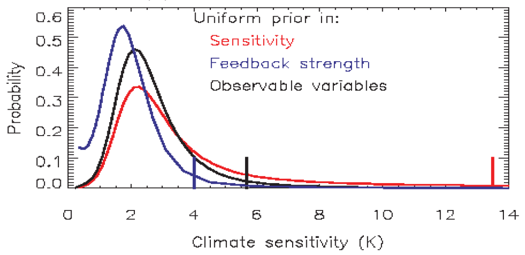 Figure 1: reproduction of Fig. (c) from Frame and Allen ‘Observational Constraints and Prior Assumptions on Climate Sensitivity’, 2004 IPCC Workshop on Climate Sensitivity. Vertical bars show 95% bounds.
However, the Frame et al 2005 claim that high sensitivity, high heat uptake cases cannot be ruled out is incorrect: such cases would give rise to excessive ocean warming relative to the observational uncertainty range. It follows that Frame and Allen’s proposal to use a uniform in ECS prior when it is ECS that is being estimated does not in fact answer the question they posed, as to what the study tells one about ECS given no prior knowledge about it. Of course, I am not the first person to point out that Frame and Allen’s proposal to use a uniform-in-ECS prior when estimating ECS makes no sense. James Annan and Julia Hargreaves did so years ago.
Frame et al 2005 was a short paper, and it is unlikely that many people fully understood what the authors had done. However, once Myles Allen helpfully provided me with data and draft code relating to the paper, I discovered that the analysis performed hadn’t actually used likelihood functions for AW and EHC. The authors had mistakenly instead used (posterior) PDFs that they had derived for AW and EHC, which are differently shaped. Therefore, the paper’s results did not represent use of the stated priors. And although, I am told, the Frame et al 2005 authors had no intention of using an Objective Bayesian approach, the PDFs they derived for AW and EHC do appear to correspond to such an approach.
Now, it is simple to form a joint PDF for AW and EHC by multiplying their PDFs together. Having done so, the model simulation runs can be used to perform a one-to-one translation from AW–EHC to ECS–Kv coordinates, and thereby to convert the PDF for AW–EHC into a PDF for ECS–Kv using the standard transformation-of-variables formula. That formula involves multiplication by the ‘Jacobian’ [determinant], which converts areas/volumes from one coordinate system to another. The standard Bayesian procedure of integrating out an unwanted variable, here Kv, then provides a PDF for ECS. The beauty of this approach is that conversion of a PDF upon a transformation of variables gives a unique, unarguably correct, result.
What this means is that, since Frame and Allen had started their ‘Bayesian’ analysis with PDFs not likelihood functions, there was no room for any argument about choice of priors; priors had already been chosen (explicitly or implicitly) and used. Given the starting point of independent estimated PDFs for AW and EHC, there was only one correct joint PDF for ECS and Kv, and there was no dispute about obtaining a marginal PDF for ECS by integrating out Kv. The resulting PDF is what the misnamed black ‘Uniform prior in Observable variables’ curve in Figure 1 really represented.
Even when, unlike in Frame and Allen’s case, the starting point is likelihood functions for the observable variables, there are attractions in applying Bayes’ theorem to the observable (data) variables (in some cases after transforming them), at which point it is often obvious which prior is noninformative, thereby obtaining an objective joint PDF for the data variables. A transformation of variables can then be undertaken to obtain an objective joint posterior PDF for the parameters. I used this approach in a more complicated situation in a 2013 climate sensitivity study,[ii] but it is not in common use.
After I discovered the fundamental errors made by the Frame et al 2005 authors, I replicated and extended their work, including estimating likelihood functions for AW and EHC, and wrote a paper reanalysing their work. As well as pointing out the errors in Frame et al 2005 and, more importantly, its misunderstandings about Bayesian inference, the case provided an excellent case-study for applying the transformation of variables approach, and for comparing estimates for ECS using:
- a Bayesian method with a uniform in ECS (and Kv) prior, as Frame and Allen advocated;
- an Objective Bayesian method with a noninformative prior;
- a transformation of variables from the joint PDF for (AW, EHC); and
- a non-Bayesian profile likelihood method.
All except method 3. estimate ECS directly from likelihood functions for AW and EHC. Since those two likelihood functions were not directly available, I estimated each of them from the related PDF. I did so by fitting to each of those PDFs a parameterised probability distribution for which I knew the corresponding noninformative prior, and then dividing it by that prior. This procedure effectively applies Bayes’ theorem in reverse, and seems to work well provided the parameterised probability distribution family chosen offers a close match to the PDF being fitted.
The profile likelihood method– an objective non-Bayesian method not involving any selection of a prior – provides approximate confidence intervals. Such intervals are intended to reflect long-run frequencies on repeated testing, and are conceptually different from Bayesian probability estimates. However, noninformative priors for Objective Bayesian inference are often designed so that the resulting posterior PDFs provide uncertainty ranges that closely replicate confidence intervals.
The ECS estimates resulting from the various methods are shown in Figure 2, a slightly simplified version of Figure 5 in my paper.
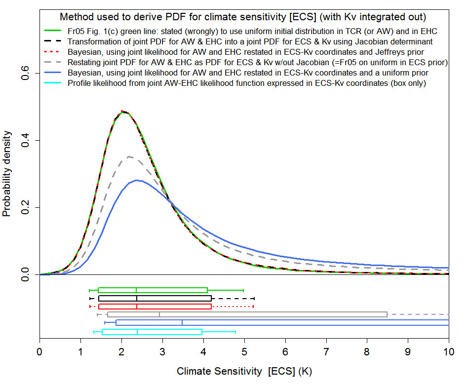 Figure 2. Estimated marginal PDFs for climate sensitivity (in K or °C) derived on various bases. The box plots indicate boundaries, to the nearest grid value, for the percentiles 5–95 (vertical bar at ends), 10-90 (box-ends), and 50 (vertical bar in box: median), and allow for off-graph probability lying between ECS = 10°C and ECS = 20°C. (The cyan box plot shows confidence intervals, the vertical bar in the box showing the likelihood profile peak).
Methods 2 and 3 [the red and black lines and box plots in Figure 2] give identical results – they logically must do in this case. The green line, from Frame et al 2005, is an updated version of the black line in Figure 1, using a newer ocean heat content dataset. The green line’s near identity to the black line confirms that it actually represents a transformation of variables approach using the Jacobian. Method 4 [the cyan box plot in Figure 2], profile likelihood, gives very similar results. That similarity strongly supports my assertion that methods 2 and 3 provide objectively-correct ECS estimation, given the data and climate model used and the assumptions made. Method 1, use of a uniform prior in ECS (and in Kv), [blue line in Figure 2] raises the median ECS estimate by almost 50% and overestimates the 95% uncertainty bound for ECS by a factor of nearly three. The dashed grey line shows the result of Frame et al 2005’s method of estimating ECS that claimed to use a uniform prior in ECS and Kv, but which in fact equated to using the transformation of variables method without including the required Jacobian factor.
For the data used in Frame et al 2005, the objective estimation methods all give a best (median) estimate for ECS of 2.4°C. Correcting for an error in Frame et al 2005’s calculation of the ocean heat content change reduces the best estimate for ECS to 2.2°C, still somewhat higher than other estimates I have obtained. That is very likely because Frame et al 2005 used an estimate of attributable warming based on 20th century data, which has been shown to produce excessive sensitivity estimates.[iii]
The noninformative prior used for method 2 is shown in Figure 3. The prior is very highly peaked the in low ECS, low Kv corner, and by an ECS of 5°C is, at mid-range Kv, under one-hundredth of its peak value . What climate scientist using a Subjective Bayesian approach would choose a joint prior for ECS and Kv looking like that, or even include any prior like it if exploring sensitivity to choice of priors? Most climate scientists would claim I had chosen a ridiculous prior that ruled out a priori the possibility of ECS being high. Yet, as I show in my paper, use of this prior produces identical results to those from applying the transformation of variables formula to the PDFs for AW and EHC that were derived in Frame et al 2005, and almost the same results as using the non-Bayesian profile likelihood method.
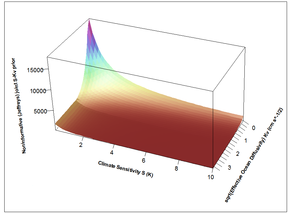
Figure 3: Noninformative Jeffreys’ prior for inferring ECS and Kv from the (AW, EHC) likelihood. (The fitted EHC distribution is parameterised differently here than in my paper, but the shape of the prior is almost identical.)
Use of a uniform prior for ECS in Bayesian climate sensitivity studies has remained common after AR4, with the main alternative being an ‘expert prior’ – which tends to perpetuate the existing consensus range for ECS. The mistake many scientists using Bayesian methods make is thinking that the shape of a prior simply represents existing probabilistic knowledge about the value of the parameter(s) concerned. However, the shape of a noninformative prior – one that has minimal influence, relative to the data, on parameter estimation – represents different factors. In particular, it reflects how the informativeness of the data about the parameters varies with parameter values, as the sensitivity of the data values to parameter changes alters and data precision varies. Such a prior is appropriate for use when either there is no existing knowledge or – as Frame et al 2005 correctly imply is normal in science – parameter estimates are to be based purely on evidence from the study, disregarding any previous knowledge. Even when there is existing probabilistic knowledge about parameters and that knowledge is to be incorporated, the prior needs to reflect the same factors as a noninformative prior would in addition to reflecting that knowledge. Simply using an existing estimated posterior PDF for the parameters as the prior distribution will not in general produce parameter estimates that correctly combine the existing knowledge and new information.[iv]
Whilst my paper was under review, the Frame et al 2005 authors arranged a corrigendum to Frame et al 2005 in GRL in relation to the likelihood function error and the miscalculation of the ocean heat content change. They did not take the opportunity to withdraw what they had originally written about choice of priors, or their claim about not being able to rule out high ECS values based on 20th century observations. My paper[v] is now available in Early Online Release form, here. The final submitted manuscript is available on my own webpage, here.
.
[i] Frame DJ, BBB Booth, JA Kettleborough, DA Stainforth, JM Gregory, M Collins and MR Allen, 2005. Constraining climate forecasts: The role of prior assumptions. Geophys. Res. Lett., 32, L09702
[ii] Lewis, N., 2013. An objective Bayesian improved approach for applying optimal fingerprint techniques to estimate climate sensitivity. Journal of Climate, 26, 7414-7429.
[iii] Gillett et al, 2012. Improved constraints on 21st-century warming derived using 160 years of temperature observations. Geophys. Res. Lett., 39, L01704
[iv] Lewis, N., 2013. Modification of Bayesian Updating where Continuous Parameters have Differing Relationships with New and Existing Data. arXiv:1308.2791 [stat.ME].
[v] Lewis N, 2014. Objective Inference for Climate Parameters: Bayesian, Transformation of Variables and Profile Likelihood Approaches. Journal of Climate, doi:10.1175/JCLI-D-13-00584.1
Postscript
James Annan had a blog post about his and Julia Hargreaves’ efforts to get their criticisms of the use of a uniform prior for ECS estimation published, here. Their paper, “On the generation and interpretation of probabilistic estimates of climate sensitivity”, Climatic Change, 2011, 104, 3-4, pp 423-436, is available here.


48 Comments
Thanks, Nic. great work
Thanks!
Nic, congratulations on getting published in the Journal of Climate. To give Frame et al some credit, they did recognize you in their acknowledgement, even if their corrigendum did not go as far as it could have.
You are right. For the record, I understand that Frame and Allen, at least, had known about the ocean heat content error since 2006, and I informed Myles Allen about the likelihood function error nearly nine months before the corrigendum was submitted. The submission and acceptance of corrigendum made my paper less acceptable for publication. Fortunately, I was able to revise my paper, cutting down what I said about errors in Frame et al 2005, so that it constituted a research article rather than being seen as a comment.
niclewis:
I’ve had a number of papers that started their life as criticisms of other people’s work:
I’ve always found that shifting the focus to original research that “exploits questions posed by previous research” has always made the paper stronger and have a longer lifetime than it would have had as a standalone criticism.
From the corrigendum: “Correcting all these errors, the upper bound of the 5–95% range for climate sensitivity under a uniform prior increases from 11.6 to 14.5°C.”
Wow
The (IIRC) 2009 Annan and Hargreaves paper you refer to has an interesting tell. Their purpose in using informed priors was to constrain the clearly implausible high ECS probability tail that results from the Frame and Allen approach, again evidenced in the corrigendum. A and H published their full resulting ECS PDFs. For both of the separately informed priors they used, the mode ECS was about 1.9 rather than 3. They never even commented on this important result.
To my knowledge, only my 2011 post at Climate Etc and the ECS discussion in the climate chapter of my last book have done so until this little comment. Certainly AR5 took no mind.
Their estimates were much closer to the newer ones you are deriving than has been generally recognized.
Thanks for your comment.
The Annan and Hargreaves paper (published online in 2009, but only in 2011 in the printed journal) compares the effects on ECS inference based on the likelihood function from Forster & Gregory (2006) of three priors for ECS: uniform, Webster (Expert) and Cauchy. All of these are informative priors, and all will bias ECS estimation to a greater or lesser extent. There is no justification for using any of these priors, IMO, and their influence means that none of the resulting ECS PDFs properly reflects the data and method used and the assumed error distributions.
The Gaussian error assumptions made in Forster & Gregory (2006) corresponded, as they pointed out in their paper, to an almost uniform-in-climate-feedback-parameter prior, which has the form 1/ECS^2 when expressed in terms of ECS. That prior – which has a shape quite unlike any of the three informative priors – was uninformative for their study, hence a uniform-in-ECS prior (on the basis of which their results were restated in AR4) was highly informative. I blogged about AR4’s distortion of the Forster & Gregory (2006) results here.
Although AR5 does not properly address the issue of informative vs noninformative priors, it does at least discuss it. And it presents the Forster & Gregory (2006) results on their original basis, corresponding to use of an uninformative prior, as well as the AR4 altered version. The median estimate comes down from 2.4 K to 1.5 or 1.6 K, and the 95% bound from 14.2 K (AR4 Table 9.3) to ~3.5 K.
The median, which is not given in the Annan and Hargreaves paper, is a better best estimate for skewed distributions than the mode, but is unfortunately more difficult to deduce from their graphs.
“The median…..is a better best estimate for skewed distributions than the mode”
That makes no sense! Did you mean to write the mode is a better estimate for skewed distributions than the mean? If not, then where do you derive this odd assertion? The mode is the ‘most probable’ value whereas the median is just the middle point between the upper and lower values and tells us nothing whatsoever about probability.
Consider what happens if you look, rather than at the distribution of a random variable x, at y=f(x), where f(x) is a monotonic transformation. For example, f=1/x. The median transforms in the expected way, as do quartiles etc. However, the mode may be in an entirely different place if f'(x) is not constant.
A simple example is the blackbody radiation spectrum. (This is an intensity distribution, not probability, to be sure, but the principle is the same.) The frequency density peaks at a photon energy of 2.821*kT; the wavelength density peaks at E=4.965*kT. [Coefficient values courtesy of Wikipedia.)
how much of the distribution falls below the median?
Well I asked a perfectly valid question yet received no reply from Nic – just two utterly irrelevant replies from others. I’m wont therefore to assume that Nic is just talking nonsense and that there is no reference or proof anywhere for this very odd assertion – merely his own gut feeling.
JamesG, you got a perfectly sensible reply from HaroldW which explained the issue clearly; that’s why nobody else felt the need to add anything further.
Jonathan Jones
That might have been a sensible reply if we were dealing with an abstract random variable but we aren’t; we intrinsically know that increasing sensitivity is decreasingly likely and the mode confirms the most probable result as being low. Using the median can give exactly the same result whether the most probable value is close to 1.5 or close to 4.5. So what he is implicitly asserting is that the skew in the distribution is unimportant.
Yet just looking at the distributions (rather than attempting to describe them by a single number) tells you the mode is more important. Use instead a median value in print and most folk seem to assume that it is the centre point of a normal distribution.
Such bold and unsupported assertions may have some validity in the financial world or otherwise where the underlying science is unknown or data is scarce but not everywhere and certainly not with climate sensitivity!
NIc, well done. is there a readily available reference that you recommend as an introduction to the topic of informative and uninformative priors? Cheers, Steve
PS – can you add a reference to Annan and Hargreaves – preferably the paper and a blogpost.
Steve, thanks. I’ve now added the references you suggest.
PS the best book on noninformative priors and objective Bayesian methods, as well as lots of other issues, is probably Bernardo, J.M. and A.F.M. Smith, 1994: Bayesian Theory. Wiley, 608pp.
A widely-cited review article that is well worth reading is Kass RE, Wasserman L (1996): The Selection of Prior Distributions by Formal Rules. J Amer Stat Ass 91 435:1343-1370.
When I was doing my PhD on mathematical modelling my supervisor encouraged me to look into Bayesian Statistics as a potentially useful tool. I couldn’t then (ca 1971) see how I could generate priors that would be defensible to a critical audience in a seminar. I take it that things have advanced in four decades, but is that problem still at the root of hesitation at adopting Bayesian methods?
Mind you, the Climate Scientists have got round the “critical audience” problem in a breathtakingly direct way.
Johnny Carson used to say of certain skits, “If you buy the premise, you buy the bit.” That seems to me the problem with Bayesian statistics as evidence: they only convince those who accept the prior as reasonable. James Annan points out that Frame’s prior of a uniform distribution on [0, 20] is completely unreasonable, since it supposes that ECS is three times more likely to be in [5, 20] than to be in [0, 5].
True. But I think the killer of a uniform distribution from [a,b] for a “non-informative prior” is that the choice of “a” and “b” as well as “uniform” are all three HIGHLY INFORMATIVE/BIASED assumptions.
Can you buy the premise that [2,3] is just as likely as [17,18] but [20.0001,999] has zero likelihood? No.
Interesting. My introduction to Bayesian statistical theory and practice was via medical pathology labs. Yes, those folk were a tough crowd if you didn’t handle the statistics properly (or correctly, depending on the critic 😛 ). That was 3 decades ago, and I’m not in that area any more, so I don’t know if things have changed much since. Perusing the medical literature suggests that while Bayesian theories and analysis is accepted, the application of it isn’t always accepted.
Nic, your threads and dissertations on Bayesian inference have been well timed with my summer of learning more about Bayesian data analyses and applications. At this point I see the results that one obtains from a Bayesian or a frequentist approach might well be the nearly the same if the data used for the likelihood calculation are large. In that case the prior will have little leverage on the posterior. On the other hand with sparse data, the use of a well-founded and perhaps theoretically based prior can give advantage to the Bayesian approach over that of the frequentist. The choice of the prior is going to have, however, a large leverage on the posterior when the data is sparse. That would appear to make a combination of relatively sparse data and an uninformed prior a less desirable choice. The book I have been reading on Bayesian inference tends to handle the subjective and informed approach to priors by suggesting that the prior be agreeable to the skeptics.
Kenneth, if the data are precise then choice of prior will usually make little difference. It is when data are poor – sparse and imprecise – that selecting an uninformative prior is particularly important, rather than less desirable, since with poor data an informative prior will have a major influence on estimation. An uninformative prior is designed to have minimal effect on inference about what is being estimated, relative even to poor data.
In problems involving estimating one or several climate system properties, the non-Bayesian signed-root log likelihood ratio method, applied to the profile likelihood, seems to provide an easy and useful cross check. If the likelihood peak location and uncertainty (confidence) bounds it provides aren’t broadly similar to those arising from Bayesian methods, the prior being used is probably quite informative.
Quite a lot of what is written in books about choice of priors is questionable.
“An uninformative prior is designed to have minimal effect on inference about what is being estimated, relative even to poor data.”
Nic, it is my consideration that the use of the uninformative prior is, like you state here, to have minimal effect on inference and is used when there is little prior knowledge of how the PDF might appear, but if one has a reasonable theoretical view of that PDF then the combination of sparse data and an informed theoretically based prior can out perform a frequentist approach.
Perhaps I am missing a subtle point here but is not the Frame and Allen use of a uniform prior (or thinking they were using it) considered an uninformed prior?
Also does not the Bayes rule allow one to use a posterior result as a prior when new data become available?
Kenneth, from what Frame and Allen put in their 2004 presentation and was in Frame et al (2005), they did think that use of a uniform prior in ECS (jointly with Kv) was uninformative when the aim was to estimate ECS itself. That was, however, incorrect. In the common case of a ‘location variable’ (where the error/uncertainty distribution is a function only of the difference between the true and the observed value of a variable), a uniform prior is indeed noninformative.
Although Bayes theorem is usually interpreted as allowing one to use a posterior result as a prior when new data become available, in the continuous parameter case doing so will generally not objectively reflect the combined information in the old data and the new data if the old and new likelihood functions have different forms. See reference (iv) (a 2013 paper of mine).
“Although Bayes theorem is usually interpreted as allowing one to use a posterior result as a prior when new data become available, in the continuous parameter case doing so will generally not objectively reflect the combined information in the old data and the new data if the old and new likelihood functions have different forms.”
The author of the book from which I am learning more about Bayesian analysis warns of different forms, but, of course, the examples in the book never have this problem. To the novice like me there are many subtle precautions in using Bayesian data analysis and that is why I have spent a lot of time this summer going over the details in a book on the subject – it is for beginners. Using the Bayesian terminology here, as you and some others have done, helps me better understand the processes.
I do not recall seeing in this thread any details on how you made calculations to obtain the posterior probabilities. You did not use a direct integration – did you? I am somewhat familiar with the Metropolis algorithm and Gibbs sampling. I have done some calculations using R2OpenBUGS with BUGS.
Nic Lewis, please ignore my question concerning the calculations of the posterior probabilities. On reading your paper and familiarizing myself with the terminology I think I know what you did.
“Transformation of variables” appear to be the same as “change of variables” used to simplify an integration.
Nic, I cannot find how, you, in your paper, or Frame/Allen or Annan/Hargreaves, in their papers linked here, determined the normalization constant required to give the posterior PDF in terms of probabilities. Is this something so simple that none of the authors described it and I am missing something here? I see you and Annan using the proportional sign in Bayes equations.
@Kenneth Fritsch
Hi Kenneth,
You wrote:
“I cannot find how, you, in your paper, or Frame/Allen or Annan/Hargreaves, in their papers linked here, determined the normalization constant required to give the posterior PDF in terms of probabilities. Is this something so simple that none of the authors described it and I am missing something here? I see you and Annan using the proportional sign in Bayes equations.”
Say the variable of interest is A, and the conditioning variable is B. The integral of the posterior pdf of A given B must be equal to unity.
If the prior pdf of A is a “proper” pdf but the likelihood function is not (it very often is defined only to yield correct proportionality relative to other realisations), then the result needs to be normalised by the constant factor given by inverse of the integral of the product of the likelihood function of B given A times the prior probability of A, integrated over the space of the A variable. This ensures that the posterior pdf of A given B is proper in the sense that it integrates to unity.
Mmm. This sounds more complicated than it was intended to be. Hope it helps.
Paul, thanks for the reply. I am aware of the requirement of a normalization constant and integration or summation to obtain it. I am confused here though. Are you saying that in the case(s) discussed here that the normalization constant is unity – and not by calculation but more by definition?
Hi Kenneth,
No, I was not saying that the normalisation constant is unity. I was saying that it needs to be calculated so that the integral of the pdf of interest is equal to unity, an essential requirement for the result to be deemed a proper pdf.
Say you work out your conditional probability function of “A given B” as the product of a likelihood function for B given A times a posterior pdf for A. There is no guarantee that this function integrates to unity. When you integrate this conditional probability function across the space of A you will generally find that you obtain a number K which is NOT equal to unity. But the integral of any pdf must equal unity. So, to convert the conditional probability function of A given B into a proper pdf, you then need to divide the function by the constant K. The result then retains the original relative properties of the A variable within the conditional probability function, but now integrates to unity, as any self-respecting pdf should.
The constant of proportionality which you asked for is given therefore by (1/K). This is “the inverse of the integral of the product of the likelihood function of B given A times the prior probability of A, integrated over the space of the A variable”, which was what I stated before. It just sounds complicated when you write it out textually. It is a straightforward routine step that generally is not over-described.
Kenneth,
Corrigendum.
My second paragraph should start with:-
Say you work out your conditional probability function of “A given B” as the product of a likelihood function for B given A times a PRIOR pdf for A.
Sorry for any confusion.
Paul, thanks again for your explanations. At my stage of learning Bayesian inference you can never get too much explanation. I understand the what you wrote here and previously. I think my communication has caused a problem here in that what I specifically wanted was the method used by Nic Lewis, and Annan for that matter, to integrate the function to obtain a normalization constant so that the graphs they present are truly PDFs and not something proportional to the PDF. You have been giving me the general reasoning and methods for obtaining the normalization constant. If the integral is complex and difficult to integrate it can be done numerically or by use a grid or one can obtain the proper PDF by using MCMC or Gibbs sampling.
Without the normalization one has something proportional to a PDF for the probability function of A|B and I would suppose that one could obtain a 95% probability range from that curve, but then one needs to integrate it in order to get the area under the curve. Perhaps in Nic Lewis’ absence here you can direct me to where these calculations were made.
Kenneth, I simply numerically-integrated the product of the prior and the likelihood function over the entire parameter space covered by the model-simulation grid, and divided that product by its integral (derived by summation over the grid). Doing so normalises the (joint) parameter PDF so that it represents a total probability of one. That this is correct can be seen upon integrating both sides of the full (not proportionate) Bayes’ theorem formula, giving one on the LHS. The method does rely on off-grid probability being very small.
Nic, I greatly appreciate yours and Paul’s patience in answering my query. I strongly suspected that you handled the integration as you describe here, but at this stage in my learning experience I was not all certain that I was not missing something simple.
The book I am just about finished reading is titled “Doing Bayesian Data Analysis” by John K Kruschke of Indiana University. He writes very upbeat and starts each chapter with a poem. The one on specifying a beta prior starts with:
I built up my courage to ask her to dance
By drinking too much before taking a chance.
I fell on my butt when she said see ya later;
Less priors might make my posterior beta.
Thanks again
Nic,
The effect of different estimates of ocean heat content OHC is noted. I’m sure I’m not alone in expressing misgivings about the accuracy of contemporaneous OHC estimates. Some estimates I’ve seen (but not checked) suggest that several thousand times the present sampling density in space would be needed to overcome the present sampling deficit, or a considerable and inconveniently long future time of sampling with present equipment.
Are you confident that the uncertainty of OHC has been properly accounted? >>>>>>>>>>>
From Wunsch et al 2014 (I do not agree with some parts of this paper)-
Detailed attention must be paid to what might otherwise appear to be small errors in data calibration, and space-time sampling and model biases. Direct determination of changes in oceanic heat content over the last 20 years are not in conflict with estimates of the radiative forcing, but the uncertainties remain too large to rationalize e.g., the apparent “pause” in warming. The challenge is to develop observations so that future changes can be made with accuracies and precisions consistent with the conventional rule of thumb that they should be better than 10% of the expected signal.
http://dx.doi.org/10.1175/JPO-D-13-096.1
Geoff, I doubt if uncertainty in the OHC change estimates is as high as uncertainty in aerosol forcing, so it’s not the prime cause of wide ranges for ECS.
If Wunsch and Heimberger (2014)’s estimate is correct, then total OHC change over 1993-2012 only equates to 0.13 W/m2 over the Earth’s surface, far lower than other estimates, which would imply ECS is lower than thought.
Thank you, Nic.
While I appreciate your essay and note its main emphasis on subtle variations of Bayesian estimation, I have long held a concern that the real errors involved in some of these climate data sets are so large that they swamp subtlety. They make me wonder if there was a need for time to be spent in refuting a paper – because the initial paper should not have been written when the errors were so large that the data meant little of significance.
Perhaps o/t, perhaps not..Go to youtube and get the “Hot Crazy Matrix”. It seems an apt name for some of the stuff we see out of the climate science factory. At any rate, it is a worthwhile, educational view. And it has a graph.
Phil
Reblogged this on I Didn't Ask To Be a Blog.
Nic,
An excellent and informative tutorial for those of us with a poor background in statistics. Thanks!
I think the arguments for using “noninformative” or “objective” priors are not airtight, although a uniform prior on sensitivity may well be unreasonable. The subthread here:
and some other comments in that thread (which was about radiocarbon dating, not climate sensitivity) seem to apply here as well.
Perhaps a simpler way of addressing this topic is to invert the question and ask “how strong would your prior have to be for you to believe x about the climate given the data?”. Let A be the event that “climate sensitivity is above the critical value x”, and let B be the data on CO2 and temperature. (For interest, you could think of x as being the level of sensitivity above which you would believe that immediate mitigation of CO2 emissions were called for.)
Then P(A|B)=[P(B|A)/P(B)]*P(A) with P(B|A) as the likelihood of the data given that sensitivity is above x and P(B) the unconditional likelihood of the data. Your estimate of [P(B|A)/P(B)] contains all your empirical techniques and assumptions. Your posterior belief about A given B is now a linear function of your prior P(A) with that ratio as coefficient and for any belief level p you can ask “How high would P(A) have to be given my estimate to make P(A|B) at least p?” You can back out how strong your prior has to be to make you alarmed or not.
To me, the fly in the ointment of this and any Bayesian approach is that the subjectivity is supposed to be confined to the choice of prior P(A). But in fact there is considerable subjectivity embedded in the part that is estimated, too, namely in the theory that is used to derive P(B|A) versus P(B|\A). (P(B) is the sum of these conditional probabilities.)
Still, I think that this inverted exercise asking how strong your prior has to be given the data for you to be able to believe x with strength p would be more productive and feed better into a policy calculus than the approach that starts with the prior.
In a situation like this, I would suggest that researchers do their analysis with several different priors and then examine the sensitivity of the results to the choice of prior. These priors should be explicitly discussed in the research as they constitute a large part of the inductive step in science.
There is some merit in showing sensitivity to choice of priors where the researcher has a rough idea of what shape a noninformative prior might be. Unfortunately, that is very unlikely to be the case in respect of priors for parameters when the relationship between the parameters and the observable variables is highly nonlinear – certainly where there are multiple parameters. All the parameter priors considered by the investigator may easily be highly informative.
In such cases, it makes much more sense to carry out any exploration of sensitivity to priors by trying different priors for observable variables What prior is likely to be noninformative in relation to observable variables is often obvious from the nature of errors and other sources of uncertainty affecting them. After carrying out Bayesian inference to obtain a joint posterior PDF for the observables, a transformation of variables can be undertaken to obtain a joint PDF for the parameters. This approach avoids the need to ascertain a suitable joint prior for the parameters.
Whether or not sensitivity to prior is investigated, I recommend comparing Bayesian results with those from a profile likelihood method, which does not involve selecting a prior and so provides objective, although not usually exact, parameter inference.
Nic,
Yet another excellent paper. Well done.
On the face of it, you are seemingly very polite to Frame and Allen 2005 here if I am following the plot correctly.
You observe that there is a “one-to-one and onto” mapping from the 2-D parameter space (S, Kv) to the 2-D observation data (Ta, “Ocean Heat”). Hence, given a postulated error range on the actual observed data, converted into a (posterior) joint pdf, the joint pdf of the actual observed data can be inverted uniquely into the parameter space using the standard approach to transformation of random variables. This gives you a joint pdf in the parameter space, from which the marginal distribution of climate sensitivity is obtained directly by integrating out the Kv term.
“The beauty of this approach is that conversion of a PDF upon a transformation of variables gives a unique, unarguably correct, result.”
Exactly.
You then go on to show that the same result can be obtained…etc, etc.
I am not in any way offering a critique of your thoughtful comparison of the different Bayesian approaches. It is just that this first result would seem to demonstrate that the Frame and Allen posterior distributions for ECS were complete and utter nonsense, unless their postulated range of values for the observables were grossly at odds with reality.
“Whilst my paper was under review, the Frame et al 2005 authors arranged a corrigendum to Frame et al 2005 in GRL in relation to the likelihood function error and the miscalculation of the ocean heat content change. They did not take the opportunity to withdraw what they had originally written about choice of priors, or their claim about not being able to rule out high ECS values based on 20th century observations.”
From the corrigendum, Frame and Allen write:-
“Correcting all these errors, the upper bound of the 5–95% range for climate sensitivity under a uniform prior increases from 11.6 to 14.5°C. “
I am completely nonplussed. Although I often disagree with Allen’s conclusions, I have generally found him to be an honest scientist within his beliefs. The acknowledged confusion over whether the distributions attributed to the observed data were posterior pdfs or likelihood functions does not change the fact that one cannot obtain a sensible observational pair with a high postulated ECS. How does Myles justify the retention of this ECS distribution?
Paul, Thanks!
Yes indeed, none of the Frame and Allen posterior distributions really made sense other than that (mistakenly) stated to use a uniform prior in the observable variables AW and EHC, but which in fact represented a transformation of a joint posterior PDF for AW and EHC.
You would have to ask Myles Allen himself how he justifies retention of the ECS distribution based on a uniform prior in ECS. I’m unsure. But, if I understand his current views correctly, he now views objective Bayesian methods less favourably than subjective Bayesian methods, although he seems to have switched from Bayesian methods to using a profile likelihood method.
Certainly, Myles Allen used profile likelihood in the Nature paper Allen et al (2009): Warming caused by cumulative carbon emissions towards the trillionth tonne. That study used the same model and observables as Frame et al (2005), but with a different, considerably higher, estimate for AW. Parameterised approximate likelihood functions were used, unlike in Frame et al (2005). The resulting 5-95% range for ECS was stated to be 2.0-4.8 K, well constrained despite a high best estimate (likelihood peak) of 3.0 K.
“I am completely nonplussed. Although I often disagree with Allen’s conclusions, I have generally found him to be an honest scientist within his beliefs. The acknowledged confusion over whether the distributions attributed to the observed data were posterior pdfs or likelihood functions does not change the fact that one cannot obtain a sensible observational pair with a high postulated ECS. How does Myles justify the retention of this ECS distribution?”
One very important aspect of the Frame and Allen choice of priors and the resulting posterior PDFs that to my awareness has not been addressed directly in this thread is that the upper bound of the 5%-95% range for climate sensitivity could have very profound effects on policy and/or campaigning for policy changes regarding government actions on AGW. The median values for sensitivity in the graph (Figure 2) in this thread, using various priors, varies closer around 2 degrees C, but the 95% upper bound varies from around 5 degrees for 4 cases to over 10 degrees for 2. The differences in the median is probably not going convince many people of a crisis but if those people were somehow convinced that there is a chance, not diminishing small, that the global temperature could change and change quickly by amounts that would make the world very different than it currently is or has been in recorded history, those people might well agree to very draconian measures in attempts at mitigation.
With this in mind I would think that scientists reporting such a PDF for very high 95% upper bounds for ECS would be very careful and sure of their calculations/estimates and prior beliefs or at least clearly point out the potential problems (sensitivities) with their estimates. When a scientific finding could so profoundly affect policy, the interested observer, I think, must also be aware of possible motivation on the part of the scientist and the effect it might have on how strongly they support their findings even in the light of counter evidence.
“Certainly, Myles Allen used profile likelihood in the Nature paper Allen et al (2009): Warming caused by cumulative carbon emissions towards the trillionth tonne. That study used the same model and observables as Frame et al (2005), but with a different, considerably higher, estimate for AW. Parameterised approximate likelihood functions were used, unlike in Frame et al (2005). The resulting 5-95% range for ECS was stated to be 2.0-4.8 K, well constrained despite a high best estimate (likelihood peak) of 3.0 K.”
“From the corrigendum, Frame and Allen write:-
“Correcting all these errors, the upper bound of the 5–95% range for climate sensitivity under a uniform prior increases from 11.6 to 14.5°C. “ ”
What am I missing here? Is it me or audacity on the part of Allen?
Kenneth, I’m not sure you are missing anything. Except perhaps that the statement in the Frame et al (2005) corrigendum would still be literally true whether or not Myles Allen believed that use of a uniform prior in ECS (and sqrt(Kv)) gave a tolerably realistic range for ECS.
4 Trackbacks
[…] claim about not being able to rule out high ECS values based on 20th century observations. My paper[v] is now available in Early Online Release form, here. The final submitted manuscript is available on […]
[…] They developed the work presented into what became an influential paper, Frame et al 2005,[i] here, with Frame as lead author and Allen as senior […]
[…] and Profile Likelihood Approaches. Nic discusses his new paper in a Climate Audit blogpost called Paper justifying AR4’s use of a uniform prior for estimating climate sensitivity shown to be f…. The paper that Nic is referring to is Frame et al. (2005), which attempted to use prior […]
[…] https://climateaudit.org/2014/07/30/paper-justifying-ar4s-use-of-a-uniform-prior-for-estimating-clima… […]