Moberg et al. [2005] use the July temperature reconstruction of Korhola et al. [2000] using Lake Tsoulbmajavri diatoms as one of 11 low-frequency proxies, as shown in Figure 4 of Korohla et al. reproduced below. There is obviously nothing in this reconstruction that is inconsistent with a pre-hockey stick view of climate history.
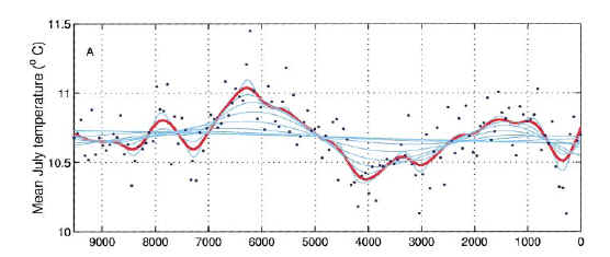 . (Original) FIG. 4. Reconstructed mean July temperatures at Lake Tsuolbmajavri for the last 10,000 years
Korhola et al. note the very strong warmth (~7000-5000BP) in the Holocene Optimum , which they associate with the maximum distribution of Scots pine in northern Fennoscandia reported elsewhere between ~6500 and 4500 BP, when the "altitudinal pine limit reached up to 200 m above the present limit", contemporary with a similar expansion on the Kola Peninsula, Russia.
They associate the maximal temperatures at the end of the warm period from 2400-900 BP with the Medieval Warm Period (about AD900 to 1300) [Lamb, 1995], noting comparable effects elsewhere:
two boreholes on the Greenland Ice Sheet (Dahl-Jensen et al., 1998) and in records from lakes (Stager et al., 1997; Rietti-Shati et al., 1998) and mires (Street-Perrott and Perrot, 1990) in Africa; it is also seen by glacier recession in different parts of the world, including Swedish Lapland (Denton and Karlen, 1973)
They associate the subsequent cooling phase with the Little Ice Age (about AD1550-1850) [Grove, 1998], noting that:
There is an increasing amount of evidence to document that subarctic and arctic lake ecosystems experienced marked changes in their limnology during the LIA event (Douglas et al., 1994; Anderson et al., 1996; Sorvari and Korhola, 1998; Korhola et al., 2000b).
The relationship between MWP and 20th century levels in this proxy is obviously different than in the Moberg proxy-only reconstruction shown here. I’m continuing the examination of Moberg et al [2005] low-frequency proxies to clarify their individual contribution to the overall low-frequency reconstruction.
Reference: Korhola, A., Weckstràƒ, J., Holmstràƒ, L. & Eràƒ⣳tàƒ P. A quantitative Holocene climatic record from diatoms in northern Fennoscandia. Quat. Res. 54, 284-294 (2000).


6 Comments
From a sampled data point of view I see a number of potential problems with this paper. The following statement under the heading, “Averaging of calibrated low-resolution temperature indicators“, is especially striking (NATURE – VOL 43 pg. 617).
“Timescales of > 340 yr are long enough to ensure that only information at frequencies lower than the Nyquist frequency for the most poorly resolved proxy series are used.”
This statement is at odds with sampling theorem. The Nyquist criterion requires that signal of interest be band limited to less than half the sample rate. If the signal of interest is not band limited, and there are frequencies greater then or equal to the sampling rate, then aliasing occurs. For example, assume we are taking samples once every second (sample frequency 1Hz). Let us also assume the signal has not been band limited and we have a frequency of .9Hz present. This .9Hz component will result in an alias which will appear in the frequency spectrum between 0 and .5Hz, as a 0.1Hz signal. Also, a frequency of 0.6 Hz would result in a alias of 0.4 Hz. In other words, any frequencies component between .5 to 1 times the sample rate would be mirrored into the 0Hz to .5Hz frequency spectra. From 1 to 1.5 times the sample rate the frequency components would create aliases but would not be mirrored. A 1.1Hz component would appear as a 0.1Hz component. Frequencies from 1.5Hz to 2Hz would again mirror as did the frequencies in .5Hz to 1Hz band and so on. The key here, and the reason for the Nyquist limit, is that when aliasing occurs there is no way to distinguish an alias from a real signal. The simple fact is there is no way to remove the aliases, the signal is irreversibly corrupted. Their claim that they “ensure that only information at frequencies lower than the Nyquist frequency” is at odds with the sampling theorem and provably wrong.
You are right about the Nyquist criterion. Perhaps by “only information at frequencies lower than the Nyquist frequency” they mean band limited? Is there anywhere I can view this paper?
Looking at the above graph and the comments “above average warming” when we are dealing variations of mean temperature within 0.5 Degree Celsius, is not what I would interpret as “warming” or “cooling” in a practical sense. We need to relate these data to human experierence, and temperature fluctuations of +/- 0.5 Deg. Celsius are imperceptible to the senses.
If we restrict the analysis to the data in hand, sure, there seems to be obvious trends but all within the resolution of a standard mercury thermometer?
I suspect our researchers have become lost in the forrest of data, forgetting that all science ultimately is used to explain human experience of reality. We cannot experience such thermal subtleties.
What is a “low frequency” proxy?
These guys import signal-processing terms. High-frequency is rapid up and down fluctuations; low-frequency is long fluctuations. Whether these are “frequencies” in a Fourier sense or simply red noise is, as far as I’m concerned, an open question. If you have fractional processes, you get “power” at all frequencies.
You’re being energetic in browsing through these old posts. It’s nice to see that they’re not lost, since some of these older posts stand up pretty well.
so what’s the implication of low frequency? Is it low noise? Why mention the term or reven move to the frequency domain at all. I mean it’s all data for a regression versus time, no? Do they actually think that there are periodic effects (waves) that are different from the noise?