Climate Audit

David Stockwell was intrigued by the seeming “robustness” of O&B results. There’s a reason for it: pretty much every one of the stereotyped Hockey Team proxies that are common to multiple studies are included in the O&B collation: bristlecones, Briffa’s re-processed series, Thompson’s Dunde and Guliya, Jacoby’s Mongolia. Pretty much every rascal has been gathered into one corral. The non-tree ring series – Chesapeake Bay, Greenland dO18 – do not show elevated 20th century results, but simply function as noise, allowing the stereotypes to dominate.

I’ve tried to do a collation of the proxy series used in O&B. There are two main problems – (1) some of the series attributed to Esper cannot be replicated using the citations: Quebec (cana169); Tirol (germ21); Mangazeja(russ067, russ068); Boreal/Upperwright. Some of the Briffa versions were previously archived at his website, but the measurements are unarchived (Tornetrask update; Yamal; Taimyr; Boreal/Upper Wright).

I’ve posted up a script to do the best collation possible for the Osborn and Briffa data http://www.climateaudit.org/scripts/osborn06.collation.txt. I’ll update this if and when more information becomes available or if I figure anything else out. I’ve tried to write it so it works externally, but I might have left in some directories and functions from my own computer – let me know if there are any issues. I’ve included a function in R to do RCS chronologies, which you hear about often and which is really very trivial mathematically. (I’ve got a slicker way of doing this using mixed effects models, but that’s for another day.) I’ve separately archived the collated proxy data at data/osborn06/osborn.txt and the annual HadCRU temperature for the applicable gridcells data/osborn06/temperature.txt. From this information, the claimed correlations between proxies and gridcell temperature can be easily tested. I’ll discuss that on another occasion.For today, I’ll report on collation issues, some of which I dealt with in my review, but which I’ll discuss more systematically here.

Provenance
O&B use 6 proxies from Mann and Jones [2003], of which 5 are in the Jones and Mann [2004] archive; and use one from from Jones and Mann [2004] attributed to Mann et al. [Eos 2003]. In terms of replication, all 6 versions can be reconciled to the illustration in O&B as shown below. Similarly, O&B use 3 proxies from Briffa’s website, which also reconcile. The 4 Esper series are a dog’s breakfast. Measurements for the Icefields (and its predecessor Jasper site) are unarchived.

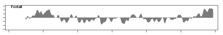
Bristlecones and Foxtails
I discussed this in my review. The comparison below shows smoothed versions of the archived MJ PC1 (which as mentioned yesterday) uses the erroneous MBH98 principal components methodology and is essentially just the Sheep Mountain site (over 80% of variance).

Series 3 described as “Boreal/Upperwright” is slyly described at realclimate today as an “independent” series, somehow affirming the validity of the PC1. However, foxtails interbreed with bristlecones and are located in the Sierra Nevadas only a short distance from Sheep Mountain. They are not “independent”. There are some real puzzles as to the provenance of this data. Esper et al. [2002] acknowledge Graumlich as having provided the data. O&B cite Llloyd and Graumlich [1997] for the data, but that article does not contain any chronologies and the sites are not referred to by the names used in Esper et al [2002]. The sites are mentioned in Bunn et al. [2005], which I discussed previously at this site. Bunn said that he has never had access to the rwl files for these sites and said that his understanding is that the files were lost when Graumlich moved to Montana in 1999. There are 5 foxtail rwl files at ITRDB from California. As an experiment, I did RCS calculations for Cirque Peak and Flower Lake (on the possibility that these might have been what Esper actually used). Especially in the later part, the chronologies are quite similar. The lack of sources by both Esper et al and O&B is maddening. Note the differences with the chronologies on the other side of the valley around 1000 and around 1200 (hash marks are 800, 1000, 1200,…)

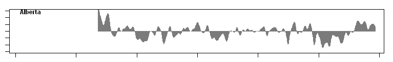
Jasper/Icefields Alberta
Rob Wilson, the author of the Icefields study, checked in today to say that I was taking too hard a line on cherry picking. Rob has been generous with his time to me and I respect his opinions. Unfortunately, he’s the low man on the food chain in the distribution of funds and he has not been allowed to archive the data from this and other studies and not even the chronology, much less the measurements, have been archived. The Icefields chronology is used by O&B to supercede the prior Jasper chronology, where the measurements were likewise not archived. Like the bristlecones, this has elevated 20th century growth, making it popular in Hockey Team studies.

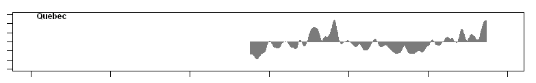
Quebec
The provenance of this series is a puzzle as I mentioned in my review. Esper et al had acknowledged data from Payette and Filion, while Briffa used the Schweingruber series cana169, terminating it in 1947 although the data goes to 1989. I did a RCS chronology from cana169 also truncating in 1947 and got similar looking results through much of the chronology, but with a rise at the end where Briffa shows a decline. It’s hard to say what’s going on.

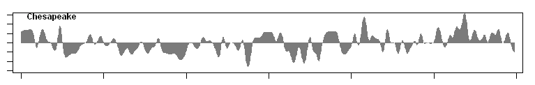
Chesapeake Bay Mg/Ca
This data set was properly archived by Cronin at WDCP in the first place and was used in Mann and Jones [2003]. O&B obviously used the JM04 version, as evidenced by the following graphics. This graphic does not show elevated late 20th century values – the opposite. In fact, the non-tree ring proxies are really just there for grandstanding.

Crete, Greenland O18
This series is popular in Hockey Team studies. It does not have an elevated late 20th century, but it is so completely lacking in low frequency variation that it doesn’t interfere with tree ring dominance. The O&B version is obviously drawn from the version used in JM04 (and MBH99 etc.)

Van Engeln Documentary
This was not used in Mann and Jones [2003], but was used in Jones and Mann [2004] and Mann et al [2003]. The O&B version is clearly identical to the JM04 version (which differs somewhat from the version archived by van Engeln at the KNMI website). It has a strong 20th century trend. It is not present in the MWP. It seems to me that including this type of “proxy” simply makes homogeneity problems worse and there is no valid reason for its inclusion, except to pad 20th century statistics and inflate perceived robustness.

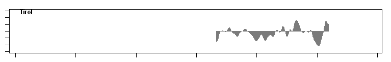
Austria (Tirol)
This situation is rather like the Quebec one. It’s an Esper series, where O&B cite an ITRDB dataset (germ21) by a different author than credited by Esper. I did an RCS chronology from the germ21 archive and got very different results than shown by O&B, who must have used something other than germ21 to obtain their results. Again this doesn’t have MWP values. While 20th century values are somewhat elevated, they are not the highest in the record. Its presence in this form seems like a nuisance.

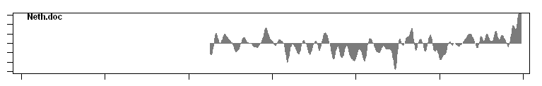
Tornetrask
There has been lots written at this site about Tornetrask – check the Jones et al 1998 category on the right frame. Tornetrask has been a staple of all studies. I’ve shown a smoothing from a series at Briffa’s website and obviously have the same version here. The swed019 dataset has a lot of data, but the Grudd measurements used here is unarchived. I’ve also showed the millennial reconstruction from Grudd, Briffa et al [2002], which says for a specialist audience: The relatively warm conditions of the late twentieth century do not exceed those reconstructed for several earlier time intervals,. If you squint at the long millennial verion, it does seem to tie together with the version used here.

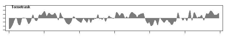
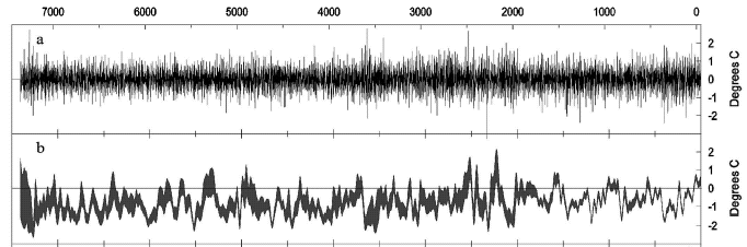
Original Caption: Figure 8 Summer-temperature variability over the last 7400 years in northern Sweden expressed as anomalies from the base period 1869–1997. (a) High-frequency variability, i.e., on a year-to-year timescale. (b) Medium- to low-frequency variability, i.e., on decadal to century timescales, with one standard error banding.

Yamal. Russia
Again, O&B used the chronology archived at Briffa’s website. The underlying measurement data set is not archived. Briffa’s chronology is a “re-processed” version of what Hantemirov et al [2002] published as shown below. This series has very elevated late 20th century closing. But compare what Hantemirov said: The more northerly tree-line suggests that the most favourable condition during the last two millennia apparently occurred at around ad 500 and during the period 1200–1300. In Briffa’s version, AD1200-1300 (to the right of the 3rd hash mark) is not notably warm. One important issue is changes in latitudinal tree line (which parallel more or less altitudinal changes elsewhere, as shown in the Hantemirov figure shown below. Shiyatov made similar observations about Polar Urals.

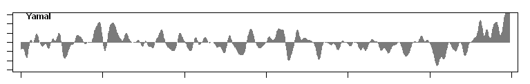
Figure 7 Corridor-standardized version of the absolute Yamal larch chronology. The units are arbitrary indices with an overall mean of 100. The histogram shown above each panel shows the number of samples incorporated at that time.

Figure 12 Regional reconstruction of polar tree-line dynamics on the Yamal Peninsula since 1800 bc. The zero line indicates the position of the recent polar timber-line.

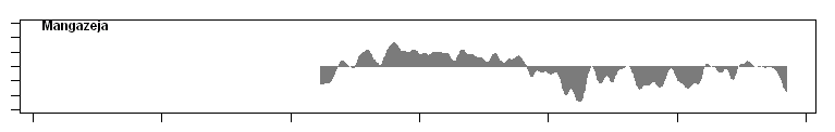
Mangazeja, Russia
This is another Esper series and like the others is unarchived and the available information inconsistent with the graphic. O&B said that they used russ067 and russ068 data sets, again Schweingruber sets, while Esper had credited someone else. There is no russ067 measurement dataset, but there are mangazpc and mangazla datasets in the Schweingruber directory at WDCP, which I used to make an RCS calculation. The two directories are of different species – spruce and larch – and it’s hard to say what Briffa did. Also the RCS calculation did not converge with a modified negative exponential model. Simply to get a value, I used a fitted cubic spline to fit the RCS calculation and got quite a different looking chronology, although the period of coverage is similar. Obviously 20th century values are not elevated. If both Mangazeja and Yamal are linear temperature proxies, I find it hard to conceive a climate model which could yield such different looking curves.

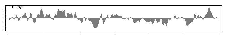
Taimyr
Again, O&B have used the chronology from Briffa’s website. This chronology shows elevated values in the early part of the 20th century. Naurzbaev: From the early ad 1960s, however, the strong warming seen in the hemisphere curve is clearly absent in Taimyr.

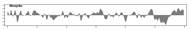
Jacoby, Mongolia
The O&B version is consistent with the version archived for JM04. This has become a popular Hockey Team proxy as it has elevated 20th century values and low MWP values. It is done by Jacoby – who has said that he only archives sites that tell a good “story”. Jacoby has provided little information on the ecology of the Sol Dav site, but other Mongolian sites analysed by their group have been described as precipitation proxies and intuitively it is hard to conceive that sites in Mongolia would not be affected by precipitation.

Yang’s China Composite
This version is properly archived and Yang promptly emailed me the constituent series when I requested. The “active ingredient” in this composite are two Thompson ice core series, Dunde and Guliya, where Yang used a grey version with 50-year averages. Until recently, Thompson had never archived these series and in late 2004, after my request, archived 10-year averages which were inconsistent with the version used by Yang. In order to reconcile this (and still further inconsistent versions of the Thompson data, a sample-by-sample archive of the Thompson data should be provided.

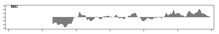
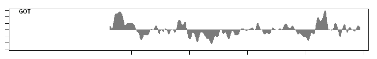
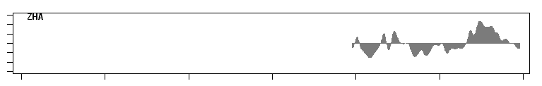
Excluded Esper Series
Here are my estimates of 4 excluded Esper series – Mackenzie Mountains, Gotland (see earlier CA posts); Jaemtland (also see earlier posts) and Zhaschiviersk. None of these show elevated 20th century values. If these were regarded as candidate proxies on an ex ante basis, then their ex post exclusion on their supposed failure to reflect local temperature requires an explanation not yet provided by O&B.

Robustness
I’ve talked from time to time about my view that a few stereotyped proxies with hockey stick shapes can impress a hockey stick shape on an multiproxy average where most of the series are simply noise. O&B argue that their results are robust because they can get pretty similar results through jack-knifing.

Readers of this blog will be familiar with certain proxies which I’ve criticized both individually and in their repeated use. So I can’t be accused of making an ad hoc response if I criticize them one more time. There are 8 proxies out off 14 with strongly elevated 20th century values that contribute the hockey stickness to O&B: the Mann PC1 (Sheep Mountain); the adjacent foxtails; Jacoby’s Mongolian site; Briffa’s Tornetrask and Briffa’s re-processed Yamal; Thompson’s Dunde and Guliya (expressed through the Yang composite); the van Engeln documentary series and Wilson’s Alberta series. There are 6 with not anomalous 20th century results: Chesapeake Bay Mg/Ca; Greenland dO18; Tirol; Mangazeja; Taimyr; and the Quebec series (although a longer version of the Quebec series does have higher values).

Obviously, there’s been lots of comment here about bristlecones, foxtails, Dunde and Guliya, Jacoby (Mongolia) and Briffa. The active ingredients here are the usual ones. The documentary record should not be used for homogeneity reasons. The non-tree ring records are clearly not active ingredients. It may be interesting that some of the most anomalous tree ring records are in mid-latitude arid environments (bristlecones, foxtails, perhaps Mongolia) and, aside from CO2 fertilization, might simply be responding to the 20th century “pluvial” in the western U.S.