Here’s Willis’ most recent summary of the ongoing dialogue on the Emanuel story.
OK, got the HadISST data … here’s the story. Emanuel used the HadISST data, smoothed three times (not four, as with the PDI data). Here’s the match:

At this point, we can do some actual analysis of the results … the three unsmoothed datasets, appended at the end of this post, have the following characteristics.
1) NONE of the three has a significant trend. The figures are as follows:
ITEM , Orig PDI , HadISST , Adj PDI
Trend z , -0.87 , 1.37 , -0.10
Kendall z , -1.26 , 1.58 , -0.62
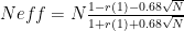
The "Trend z" is the significance of the trend, using Nychka’s adjustment for autocorrelation:
The "Kendall z" is the significance of the trend, using Kendall’s non-parametric trend test. 2) The SST is related to both the adjusted and unadjusted PDI, as follows:
ITEM , Orig PDI vs HadISST , Adj PDI vs HadISST
r^2 , 0.21 , 0.25
p value , 0.01 , 0.002
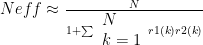
The p value has been calculated using Bartletts formula for the effective N,
While these relationships are statistically significant, they are quite small.
3) The method of smoothing (pinning the end points and repeatedly using a 1-2-1 smoothing filter) distorts the results. By pinning1) While there is a significant trend in the HadISST in the area from 1949-2003, there is no significant trend 1931-2003.
4) While there is a small relationship between the September HadISST sea temperature and the original PDI (r^2 = 0.21, p = 0.01), the relationship drops to r^2 = 0.08, p=0.12 when we use the August to October HadISST sea temperature … looks like my original suspicions of cherry picking were correct.
5) the endpoints, the start and finish of the curve are held in place, and the smoothed curve is adjusted to meet them. Because the start and end points are low and high respectively for both the PDI and the SST, this converts a "U" shaped curve into more of a hockeystick shape, by pinning the start low and the end high …


65 Comments
I think there is a type in Nychka’s adjustment. It should be (1-r-.68/sqrt(n))/(1+r+.68/sqrt(n))
That makes 5 major provable sources of cherry-picking:
-SST time-framing
-storm & SST spatial framing (the “box”)
-the 30-year time-frame of analysis and title of paper
-super-smoothing to exaggerate subdecadal (not trend!) coherence
-conscious decision to retain end points during smoothing, thus keeping the HS blade trend intact (reported in Landsea communication arising, but not understood for its full effect)
And one wrong conclusion:
-Much of the r^2 is attributable to ENSO-scale coherence, NOT the warming trend
It is possible to separate out the effect of each (ENSO vs W) through the use of orthogonal filters. My a priori guess is Emanuel’s warming trend cofficients will be cut in half, possibly much more.
Willis, Nychka’s correction method is for AR1 processes. By the time all the 3x and 4x smoothing is done, the SST and PDI data are no longer AR1 processes, they have become truly cyclic AR2 processes, with AR1 > 0 and AR2
At this point, re: TCO’s urging, I suggest we write a paper:
“Hurricane response to ‘warming’ in the Atlantic basin: a sensitivity analysis”
with Judith Curry being the lead writer and Willis Essenbach and myself as the lead analysts. (Single quotes around “warming” optional :)) What do you say?
The idea would not be to refute Emanuel, but to explore how different choices during analysis lead to different flavors of outcomes.
This would be a gentle way of highlighting the problems with choices such as not lopping of the endpoints during smoothing of a non-stationary series (generated by a possibly stationary stochastic process). And it would be a demonstration of that principle – what’s that phrase? – “death by a thousand cuts”? Something like that.
I haven’t followed all the thread, but why not focus on attacking the statement that hurricane power dissipation has doubled, ultimately by providing an correct (and much lower if not insignificant increase) estimate of the increase in power dissipation?
Because that would be exactly that – an attack, not an analysis. Rest assured, this will be one key element of a more coherent analysis, as mentioned earlier in the thread.
Attacks are destructive, and hard to publish. Syntheses are helpful, and easy to publish.
Although … it might be advisable to publish 2 papers, a communication arising: “Have hurricane intensites in recent decades doubled?”, followed by a more substantive synthetic paper, as susggested above. The optimal strategy will depend on the final results, which we’ll have tonight, and consensus opinion at CA. Let’s hear what Judith Curry has to say.
Falsification is essentially an attack on claims and the only really reliable and effective scientific method. I don’t think one should shy from hard to publish papers, its a problem with the system not the analysis. This is encouragement not criticism.
Re #9
Point taken, as indicated in #8. My point is that there is an important semantic distinction to be made between “falsification” and “attack” which is critical in the academic world. This analysis will not fully falsify Emanuel’s primary hypothesis. It will merely downgrade his estimates. I would prefer to elighten the community than to attack any one person. This is my last post on the issue until Judith and Willis weigh in.
Analysis of the raw unsmoothed data indicates Emanuel did not need to smooth the data at all, or cherry-pick the start date to obtain p |t|)
(Intercept) -339.878 82.259 -4.132 0.000129 ***
SST 12.540 2.944 4.260 8.4e-05 ***
—
Signif. codes: 0 `***’ 0.001 `**’ 0.01 `*’ 0.05 `.’ 0.1 ` ‘ 1
Residual standard error: 5.711 on 53 degrees of freedom
Multiple R-Squared: 0.2551, Adjusted R-squared: 0.241
F-statistic: 18.15 on 1 and 53 DF, p-value: 8.406e-05
So … why did he do it?
-To improve the optics on the graphics?
-Because he didn’t know how else to estimate the amount of temperature-related increase in hurricane intensity?
Downgrading of initial estimates and certainty seems to be a consistent theme in climate studies.
Look at what is happening with estimates of 2xCO2 sensitivity, CO2 emmissions, and its a substantive and important result in itself. Good luck!
I agree that “we” (somewhat loosely defined at this point) should write a paper or two on this. If your analysis shows that you can falsify the hypothesis that “hurricane intensity is increasing since 1970 (or from 1944 or whenever)”, then that should definitely be a paper. I don’t think (?) you can totally falsify the hypothesis that there is an increase (we will see), so the more likely alternative paper would be on the sensitivity of drawing conclusions about the magnitude of the increase to various assumptions re smoothing, selecting SST data, starting point, showing all the statistical significance tests and what kinds of conclusions can be drawn re trends, correlations, etc
in terms of authorship, the person who actually writes most of the text should be first author. If the text is dominated by statistical content, I should not be first author (we all agree that i am no expert on statistics), but i could certainly play a major role in writing the intro/conclusion type stuff and framing the general content of the paper. On the other hand, if the other authors are allergic to writing, then I could take the lead. But i think willis or bender would be better as first author. We can figure this out later. My preference would actually be last author, indicating a collaborative and oversight role rather than an instigating role. On the other hand, depending on where we decide to submit this, having me as first author might help grease the way a bit.
How is this for a title: Auditing the statistical analysis of trends in tropical cyclone activity
I like using the word “audit” for several reasons, besides the obvious trademark of this blog. What is going on here (this discussion on climateaudit) is important in the context of the sociology of science. A group of people (some of whom we don’t even know what their real names are), who don’t have any funding to this and are working outside the mainstream of the scientific establishment, have motivated due diligence, or auditing on this research, and one of the mainstream researchers is collaborating with them (certainly a different interaction than the hockey stick brouhaha), and they actually accomplish something that moves the science forward. sort of a “flat world” approach to science.
Here is another idea for a paper (i would probably need to write this one by myself): Spinning climate science in the blogosphere, for BAMS or something like that
Ah, a Bayesian! Welcome, all Bayesians. Being open to the idea of having your priors adjusted by out-of-sample data, you may want to prepare for a downgrading.
#14 was a crosspost in response to #12.
13:
I wonder if Dano needs to offer a bet to ensure the idea presented actually happens.
Best,
D
Re #13
Great – let’s do it! Essenbach, Dershowitz, Curry. Who else? I’ll post up some more results tonight and we can hash through it all. Do we want to do this publicly (as a demo of the collaborative process)? We would probably need to ask Steve M’s permission, as this is awfully parasitic of us to use his blog.
Using the word “audit” in the title is a good idea for the reasons you suggest. We can hash out a title once the full results are posted. Once the writing is done I will post an R script for the analysis. (I’m not sure if you use R. There is a link to it in the right-hand column, under “pages”. The script will be designed so that it would work in S+ as well.)
Re #16
I bet not.
Re #13
Forgot to say: I agree 100% with this prediction, at least insofar as the current data are concrened. (As with AGW, the effect is undeniably non-zero, positive. The question is “what is its magnitude and uncertainty?”)
If we want to examine other (1) temporal windows for computing SST or (2) spatial boxes for computing SST & PDI, then I’m less certain of the outcome. Both would be interesting. It’s up to Willis if he wants to go that extra mile.
For a paper, you people writing it would have to decide where to limit the subject matter, but for this blog I think (1) and (2) from above are just as important to the total picture as what you are currently considering.
It has been suggested here and in the Landsea communications that applicability of the PDI as a measure of potential damage or simply as a physical intensity measurement also needs to be studied further. Bender, you mentioned insurance companies and there interest in this information more than once in this thread and Landsea and Pielke have made reference to PDI and landfall hurricane damage. Is there any information that insurance companies have and are willing to divulge that would add to the discussions? After all they have more than professional reputations at stake.
Hopefully it is not too much a waste of bandwidth to reply to a direct question.
I don’t know the answer, Ken. They’d be negligent to their stockholders to not be doing investment risk assessment & risk management, including gathering & analysing data, &/or offloading risk onto unsuspecting re-insurers. I doubt they would divulge any proprietary trade secrets.
Nychka adjustments posit an AR1 strucutre, but all temperature data sets that I’ve seen ahave highly significant ARMA(1,1) structures. In the SST series posted up by Willis, the AR1 coefficients is 0.3475, but modeled as ARMA(1,1), it is (.9065, -0.7013) which is getting into some tricky regression territory.
The arima structure of the PDI data is quite different as shown below, with an insignificant coefficient modeled as AR1, but highly significant ARMA(1,1), but, in this case, anti-persistent (-0.5762,0.7738):
a
The trends of the two series according to Willis’ data have slightly different signs; the residuals from a regression of PDI on SST have the same arima structure as the predictand PDI – also note the pattern in the plot of residuals shown in the diagram below:
Steve, from you’re regression lines one might conclude that sea surface temperatures is positively correlated with pdi for some parts of the frequency spectrum and negatively correlated with pdi for other parts of the frequency spectrum.
The residuals have an AR3 structure.
I still don’t understand how to interpret the MA1 term in ocean science (or atmposhere for that matter). Is this the effect of water of a different temperature coming in from a different area and piling up in a given area of measurement, so that the temperature is effectively a sample of a truly-moving truly-averaging process? And the AR1 less than zero represents the water moving out? Like an ENSO circuit?
Open musing here. Apologies for bandwidth wastage. (Tell me if it’s unwelcome.)
An Emanuel/Mann paper worthy of some statistical deep-diving is
http://www.discover.com/images/issues/aug-06/eoshurricanes.pdf#search=%22mann%20emanuel%20hurricane%22
Re #23
That’s already been noted in yesterday’s thread, and is what underlies the statement in #2. But feel free to quantify if you wish. (Such a low negative correlation extending over the full length of the time-series is probably insignificant, however.)
#28 I agree the low negative correlation is probably not statistically significant. More data would be needed to see if ocean temperatures have a different correlation for really low frequencies like 50 year cycles.
Actually don’t see much autocorrelation in these SST data using PACF and lag plots. It should be formally tested. This is my first try at images:
See Options for ACF in R for more on PACF.
See 2000 Years Surface Temperatures Time Series Lag Plot for more on lag plots.
Re #28
The first lag is highly significant, the 3rd & 8th marginally so. The others not. Filter them as Emanuel did and you’ll inflate them. “Formally tested?” You just did the formal test. Congratulations!
#29. Yes, seems if you filter anything you make it autocorrelated. But looking at the raw data, the PACF can indicate the order of AR model that should be used. Partial autocorrelation is estimated by fitting autoregressive models of successively higher orders up to the lag.max. So I think 3 and 8 on the image are actually the significance of AR(3) and AR(8) models, not indications of high lag 3 and lag 8 correlations on an AR(1) model as you get with an ACF plot. I just mean a DW test rather than a plot to be sure. Hope this is helpful.
Depends on the filter.
Not to be insulting or discouraging, but this is actually more harmful than helpful. It’s great that you are using the tools, but like any tool you have to understand how it works to use it effectively. There are lots of cases where these tools don’t deliver “as advertised”. It takes a lot of training to know what tools to use in any given situation, because the number and diversity of tricky situations is enormous.
RE my #25
Compare Emanuel’s Figure 1 (above, from Willis) with the Figure 2 in the Mann/Emanuel paper (linked above in #25). Both are for the same data (SST for August-October, in Emanuel’s SST box).
In Figure 1, the smoothed SST blade heads for the sky about year 2000. In Mann/Emanuel Figure 2, the smoothed SST blade heads for the sky in the early 1990s.
Remarkably, the two different take-off points happen to match the rises in the accompanying plots of PDI and storm count, respectively.
If there’s an explanation for choosing different smoothing techniques in different papers for the same SST data, I haven’t found it. I will kepp reading…
Re #32
The SST series are not that different IMO. Looks like the Mann & Emanuel paper maybe did a lot more smoothing. But who knows what were done to the endpoints? Keep reading. Note that “pinning effect” or “anchoring effect” is quite strong. It makes a big differene if and when you leave/put the endpoints in.
Good luck guys. My impression is that Bender would do the best job writing the paper and being in charge of the text. Judy would be a sound last author, advisor type. Willis has done a lot of the work and may deserve high billing (not sure, haven’t kept track.)
Hey Benderino, please ignore the itsy bitsy attemptsies of the cutesy writing man to distract. I can see swatting, but not replying.
Re #35
Thanks for the reply, Ken. You never know.
Here is the (big) change in correlation as the Emanuel data are progressively smoothed, 0x, 1x, 2x. (Here I exclude the endpoints, which is what one ought to do.)
> cor(SST,PDI)
[1] 0.5050575
> cor(SST.1,PDI.1)
[1] 0.6278249
> cor(SST.2,PDI.2)
[1] 0.7484223
Square those to obtain r^2.
Next, I will show the effect on SST and PDI PACFs and spectra.
After that, regression statistics.
Stay tuned … unless you think this is wasted bandwidth. In which case please read some of the other very interesting threads being woven at CA.
Willis, your data collation starts in 1949, while the Emanuel graph for SST starts in ~1930.
#36 keep it up. I am reading these hurricane threads far more closely then the other threads lately.
Re #38
John, if you wanted to come up with a pair of orthogonal filters that could be used to separate out the low and high frequency variability in a time-series (using, say, 11-15y as the 50% cutoff), that would be a real time-saver. I’ve done it before, could do it again, but you seem so keen on that angle. (If you don’t have time, that’s ok.) If we use it in the paper (and I’d like to) you would get due credit, of course.
I’m trying to do other things but don’t seem to be motivated and this is more fun. Here is what I think you might be looking for:
A high frequency filter with the same cutoff as Emanuel
A low frequency cutoff of 11-15 years.
Zero phase distortion or time delay (non causal)
Zero gain distortion in the cutoff band
No auto regressive part
A filter length the same as Emanuel.
All these requirements can’t be met exactly be we can do a best mean squared error fit. I can right a script to find the optimal requirements for such a filter. Am I right about the requirements you’re looking for?
Sometimes smoothing the data can allow you to see trends that are not apparent in the raw data. As a layman who has built models and as a supervisor who has had employees build models, I have seen everything from remarkable insight to completely irrational conclusions to near-fraud displayed with smoothed trended data.
I always go back to the raw data to check whether remarkable insight, irrationality, is what has occurred.
Raw data plots are what needs to be shown here. In my opinion, the raw data shows some correlation (it is rational given one would expect PDIs to increase with SST) but there is no long-term trend that is evident.
Re #40
Working on other things! Ha! Tell me about it 🙂
-Characteristics 1-4, yes, exactly.
It’s not necessary that the filter be comparable to Emanuel’s in any way. This is actually for filtering the filtered data streams, so that we can do a two-phase regression, one on the low-freqeuncy SST/PDI signals, one on the ~decadal signals.
You ARE a gem. And not the fake-o kind!
I believe that we are ok in terms of collaborating on the blogosphere, but once a paper is submitted any of the graphs/text that are included in the publication should probably be pulled from the blog. Science and Nature are very picky about this, but i think the other journals are less strict about this sort of thing (and blogospheric collaborations are a new gray area, probably doesn’t count as published but would certainly violate the press embargo conditions that nature and science set, but that AGU and AMS journals don’t care about). Personally, i think the spirit of GRL is more appropriate for our proposed publication (assuming we can keep this within their page limits).
Re #43
Good point, Judith. I agree.
Judy, GRL has an “L” in it.
To me the following Willis E. comment from the lead into this thread is a huge discovery if I understand it correctly. The PDI data was gathered and used for each complete tropical storm season. Correct? So it might appear that the use of the August to October SST data would have been more appropriate to use for the r^2 regression unless most of the storms occurred in September. Can it be readily determined what percentage did occur in the month of September over this time period? On the other hand, one could have more unambiguously limited the tropical storms data (PDI) to September.
Re #46 Agreed, Ken. That’s point 1 of post #2. Nothing will be missed.
#42 Bender, I’ll tell you what. I’ll give you two sets of filters. One set with the same number of coefficients as Emanuel’s 3 times smoothing filter. One filter in this set will give the low frequency part of the filtered data and the other par will give the higher frequency part of the filtered data. The point of this filter is to get a similar effect as Emanuel’s filter but not having to drop more end points.
The other filter set I’ll give you will be two 5 moving average coefficient symmetric filter. One filter to separate the high frequency band another filter to separate the low frequency band. This will be to split the data as you say after applying Emanuel’s filter. With regards to splitting a signal and then identifying trends, I suggest subtracting the mean and then squaring before doing a linear regression fit. The reason being is squaring gives the power of the signal. If you apply linear regression to a band passed signal then the linear regression is going to favor the low frequency part of the signal when what you are interested in is how the power of signal changes with time over pass band region.
I was aware of your summary in #2, but I think that while the other “selections” you noted could make the published relationship significantly less dramatic it is this one alone, I believe, if more appropriate with ASO SST data that, essentially, would say there is no relation.
And will the second set be orthogonal, so that when I add filtered components 1 & 2, I will get the original data stream? Actually, erase that. In the case of a two-filter system, you only need to define one filter! The other will be implicit when you do the subtraction: original-filtered=complement. Duh.
Before I go to bed now, I must comment that the Willis E graphs are very easy to read and that becomes very important to older and tired eyes. Thanks Willis.
Re #49
Again, I agree. This point was made before as well in #19. That’s why I said “isofar as …”. In my view it is up to Willis et al. to decide if we want to go that extra mile. But your vote counts too.
Re #51
These crude graphs are hard to read for a reason. This way they will need to be significantly reformatted before publication.
#50 I was kind of thinking of the subtracting but wasn’t somehow necessary it was. It may be possible to get better pass band characteristics if perfect orthogonally isn’t required. However, it should be possible to optimize the filter so that the filter gives as close a fit possible to the desired characteristics of both it’s pass band and the pass band of the orthogonal filter you described. So for the two filter system we will define the orthogonal filter by subtraction as you suggest.
Re #54
Perfect orthogonality in this case is required because we want a clean, black & white hypothesis test of attribution to GW trend vs. NAO cycle.
Thanks for your contribution.
Man, this sucker is getting long, I’ll need some time to read it … go away for a couple hours, and wham! … in the meantime, a few notes.
Regarding the Emanuel-Mann paper in #25, a very quick read finds a very quick oddity … the MDR (main hurricane development region) is listed as 6°N”¢’¬?18°N, 20°W”¢’¬?60°W. They say they are using the HadSST2 database for the temperatures in this area … but the HadSST2 database is a 5° x 5° grid. From their website:
So how are they getting the SST of the MDR from that?
In #32, David, you comment about the difference between the SST in the Emanuel paper and the Mann-Emanuel paper. I assume it is because they are using two different temperature sets (HadSST2 and HadISST1), and they are using different areas (they can’t use HadSST2 for a 6°”¢’¬?18°N, it’s a 5° x 5° grid dataset).
Re the SST data you mention in # 37, Steve M., I have it back to 1931, I just didn’t post it. I actually have it back to 1870, but I haven’t extracted it.
I’m more than happy to collaborate on a paper for this, but bender will have to do the heavy statistical lifting …
w.
Oh, yeah. They’re getting cagey in the new Mann-Emanuel paper. They say:
Regarding the “addional material”, they say:
But when you go to the “addional material”, there are no details about how they’ve done the “decadal smoothing” …
Regarding the existence of this new paper, my concern about writing about the Emanuel paper is that they’ll say “oh, that doesn’t matter, we’ve moved on, see our new paper” …
w.
Re 46, I should never post after midnight. I said:
This was actually the relationship and data for the October HadISST data, not August-October. The August-October data does show a drop, but nowhere near as large (r^2 = 0.18, p=0.02).
w.
Re 59, I finally found their smoothing information, right where they said it would be, just one step further, at http://www.meteo.psu.edu/~mann/eos06/MannEmanuelEosSupplementaryInformation.pdf … it’s a Butterworth filter with Mann’s improper way of treating the cutoffs at the end … he pins the end points.
w.
Re #58
So that would put the August-only SST relationship somehwere near r^2 ~= 0.16?
For the core analyses I suggest we stick with September SST, with the month-by-month & aggregate correlations as a by-line. (The cherry-picking of September is hard to argue with. It’s probably the stormiest month. It is the middle month.)
Although I guess the real question one ought to ask is what is the August SST-PDI, September SST-PDI, October SST-PDI, with PDI computed monthly instead of aggregated seasonally. I don’t think we need to go there. Not yet. The spatial extent issue looks to be a little less robust and worthy of some prodding.
For the two system filter try the filter here:
http://www.geocities.com/s243a/warm/huricane_filter.htm
If you need a sharper cutoff I’ll see what I can do but there will probably be a price to be paid somewhere else. The code is at the bottom of the link. The filter is linear phase (zero phase distortion). I chose a 15 year cutoff to try to effect the 5 year cycle as little as possible.
I didn’t use the subtraction suggestion because just because the two outputs add up to the original signal does not mean they are orthogonal. As far as how clean it is, the low pas filter does a very good job at attenuating the 5 year cycle. The high pas filter gets rid of about half the low pass signal. I think we can increase the order of the high pass filter because it has a pretty sure impulse response.
In the link I provided I gave all the filter coefficients for high and low pass filters from order 2 to order 22. I argue that we should use the highest order filter possible. I am not sure how many end points to keep but it is possible to keep all end points in a regression analysis but weight the center points more then the end points. Thus when you plot the trend the endpoints will not have as much effect on the trend line even though they may show a sudden spurious change one way or the other.
I’m working on a table to better understand what is happening at the end points. You can see that near the end points the filter is no longer symmetric and highly dominated by the end point. If you pick the end point at the end of the 5 year cycle you will highly bias you’re filtered results at the end point.
yn  y(n-1)       y(n-2)       y(n-3)       y(n-4)       y(n-5)

-----------------------------------------------------------------

yn  y(n-0)/4     y(n-1)/4     y(n-2)/4     y(n-3)/4     y(n-4)/4

   2y(n-1)/4    2y(n-2)/4    2y(n-3)/4    2y(n-4)/2    2y(n-5)/4

yn  y(n-2)/4     y(n-3)/4     y(n-4)/4     y(n-5)/4     y(n-6)/4

-----------------------------------------------------------------

                 y(n-0)/16    y(n-1)/16    y(n-2)/16    y(n-3)/16

yn 5y(n-0)/16   4y(n-1)/16   4y(n-2)/16   4y(n-3)/16   4y(n-4)/16

   6y(n-1)/16   6y(n-2)/16   6y(n-3)/16   6y(n-4)/16   6y(n-5)/16

   4y(n-2)/16   4y(n-3)/16   4y(n-4)/16   4y(n-5)/16   4y(n-6)/16

    y(n-3)/16    y(n-4)/16    y(n-5)/16    y(n-6)/16    y(n-7)/16
Not sure how to display this write as your code tag is not displaying mono space font or it is eating extra spaces.
Somehow I missed #61-#63.
Thanks John Creighton! Will have a look.
#99 Bender I posted a suggested filter a while ago here:
http://www.climateaudit.org/?p=824#comment-47523
Since no one responded I got board with it. I have been reading more internet stuff on world events lately then global warming. Well….that and getting a lot of exercise. Thinking of the students comments about the blog being a black hole of time, it takes me a lot of time to even keep up with the hurricane threads here let alone all the thread in general. This is a very active blog and if you are not here all the time you can miss alot. No wonder the students are reluctant to participate. When you read a paper the material is much more focused and therefore arguably a more efficient use of ones time. Of course focused means narrow in scope and thus not always superior.