This is a guest post by Ross McKitrick. Tim Vogelsang and I have a new paper comparing climate models and observations over a 55-year span (1958-2012) in the tropical troposphere. Among other things we show that climate models are inconsistent with the HadAT, RICH and RAOBCORE weather balloon series. In a nutshell, the models not only predict far too much warming, but they potentially get the nature of the change wrong. The models portray a relatively smooth upward trend over the whole span, while the data exhibit a single jump in the late 1970s, with no statistically significant trend either side.
Our paper is called “HAC-Robust Trend Comparisons Among Climate Series With Possible Level Shifts.” It was published in Environmetrics, and is available with Open Access thanks to financial support from CIGI/INET. Data and code are here and in the paper’s SI.
Tropical Troposphere Revisited
The issue of models-vs-observations in the troposphere over the tropics has been much-discussed, including here at CA. Briefly to recap:
- All climate models (GCMs) predict that in response to rising CO2 levels, warming will occur rapidly and with amplified strength in the troposphere over the tropics. See AR4 Figure 9.1 and accompanying discussion; also see AR4 text accompanying Figure 10.7.
- Getting the tropical troposphere right in a model matters because that is where most solar energy enters the climate system, where there is a high concentration of water vapour, and where the strongest feedbacks operate. In simplified models, in response to uniform warming with constant relative humidity, about 55% of the total warming amplification occurs in the tropical troposphere, compared to 10% in the surface layer and 35% in the troposphere outside the tropics. And within the tropics, about two-thirds of the extra warming is in the upper layer and one-third in the lower layer. (Soden & Held p. 464).
- Neither weather satellites nor radiosondes (weather balloons) have detected much, if any, warming in the tropical troposphere, especially compared to what GCMs predict. The 2006 US Climate Change Science Program report (Karl et al 2006) noted this as a “potentially serious inconsistency” (p. 11). I suggest is now time to drop the word “potentially.”
- The missing hotspot has attracted a lot of discussion at blogs (eg http://joannenova.com.au/tag/missing-hot-spot/) and among experts (eg http://www.climatedialogue.org/the-missing-tropical-hot-spot). There are two related “hotspot” issues: amplification and sensitivity. The first refers to whether the ratio of tropospheric to surface warming is greater than 1, and the second refers to whether there is a strong tropospheric warming rate. Our analysis focused in the sensitivity issue, not the amplification one. In order to test amplification there has to have been a lot of warming aloft, which turns out not to have been the case. Sensitivity can be tested directly, which is what we do, and in any case is the more relevant question for measuring the rate of global warming.
- In 2007 Douglass et al. published a paper in the IJOC showing that models overstated warming trends at every layer of the tropical troposphere. Santer et al. (2008) replied that if you control for autocorrelation in the data the trend differences are not statistically significant. This finding was very influential. It was relied upon by the EPA when replying to critics of their climate damage projections in the Technical Support Document behind the “endangerment finding”, which was the basis for their ongoing promulgation of new GHG regulations. It was also the basis for the Thorne et al. survey’s (2011) conclusion that “there is no reasonable evidence of a fundamental disagreement between models and observations” in the tropical troposphere.
- But for some reason Santer et al truncated their data at 1999, just at the end of a strong El Nino. Steve and I sent a comment to IJOC pointing out that if they had applied their method on the full length of then-available data they’d get a very different result, namely a significant overprediction by models. The IJOC would not publish our comment.
- I later redid the analysis using the full length of available data, applying a conventional panel regression method and a newer more robust trend comparison methodology, namely the non-parametric HAC (heteroskedasticity and autocorrelation)-robust estimator developed by econometricians Tim Vogelsang and Philip Hans Franses (VF2005). I showed that over the 1979-2009 interval climate models on average predict 2-4x too much warming in the tropical lower- and mid- troposphere (LT, MT) layers and the discrepancies were statistically significant. This paper was published as MMH2010 in Atmospheric Science Letters
- In the AR5, the IPCC is reasonably forthright on the topic (pp. 772-73). They acknowledge the findings in MMH2010 (and other papers that have since confirmed the point) and conclude that models overstated tropospheric warming over the satellite interval (post-1979). However they claim that most of the bias is due to model overestimation of sea surface warming in the tropics. It’s not clear from the text where they get this from. Since the bias varies considerably among models, it seems to me likely to be something to do with faulty parameterization of feedbacks. Also the problem persists even in studies that constrain models to observed SST levels.
- Notwithstanding the failure of models to get the tropical troposphere right, when discussing fidelity to temperature trends the SPM of the AR5 declares Very High Confidence in climate models (p. 15). But they also declare low confidence in their handling of clouds (p. 16), which is very difficult to square with their claim of very high confidence in models overall. They seem to be largely untroubled by trend discrepancies over 10-15 year spans (p. 15). We’ll see what they say about 55-year discrepancies.
The Long Balloon Record
After publishing MMH2010 I decided to extend the analysis back to the start of the weather balloon record in 1958. I knew that I’d have to deal with the Pacific Climate Shift in the late 1970s. This is a well-documented phenomenon (see ample references in the paper) in which a major reorganization of ocean currents induced a step-change in a lot of temperature series around the Pacific rim, including the tropospheric weather balloon record. Fitting a linear trend through a series with a positive step-change in the middle will bias the slope coefficient upwards. When I asked Tim if the VF method could be used in an application allowing for a suspected mean shift, he said no, it would require derivation of a new asymptotic distribution and critical values, taking into account the possibility of known or unknown break points. He agreed to take on the theoretical work and we began collaborating on the paper.
Much of the paper is taken up with deriving the methodology and establishing its validity. For readers who skip that part and wonder why it is even necessary, the answer is that in serious empirical disciplines, that’s what you are expected to do to establish the validity of novel statistical tools before applying them and drawing inferences.
Our paper provides a trend estimator and test statistic based on standard errors that are valid in the presence of serial correlation of any form up to but not including unit roots, that do not require the user to choose tuning parameters such as bandwidths and lag lengths, and that are robust to the possible presence of a shift term at a known or unknown break point. In the paper we present various sets of results based on three possible specifications: (i) there is no shift term in the data, (ii) there is a shift at a known date (we picked December 1977) and (iii) there is a possible shift term but we do not know when it occurs.
Results
- All climate models but one characterize the 1958-2012 interval as having a significant upward trend in temperatures. Allowing for a late-1970s step change has basically no effect in model-generated series. Half the climate models yield a small positive step and half a small negative step, but all except two still report a large, positive and significant trend around it. Indeed in half the cases the trend becomes even larger once we allow for the step change. In the GCM ensemble mean there is no step-change in the late 1970s, just a large, uninterrupted and significant upward trend.
- Over the same interval, when we do not control for a step change in the observations, we find significant upward trends in tropical LT and MT temperatures, though the average observed trend is significantly smaller than the average modeled trend.
- When we allow for a late-1970s step change in each radiosonde series, all three assign most of the post-1958 increase in both the LT and MT to the step change, and the trend slopes become essentially zero.
- Climate models project much more warming over the 1958-2012 interval than was observed in either the LT or MT layer, and the inconsistency is statistically significant whether or not we allow for a step-change, but when we allow for a shift term the models are rejected at smaller significance levels.
- When we treat the break point as unknown and allow a data-mining process to identify it, the shift term is marginally significant in the LT and significant in the MT, with the break point estimated in mid-1979.
When we began working on the paper a few years ago, the then-current data was from the CMIP3 model library, which is what we use in the paper. The AR5 used the CMIP5 library so I’ll generate results for those runs later, but for now I’ll discuss the CMIP3 results.
We used 23 CMIP3 models and 3 observational series. This is Figure 4 from our paper (click for larger version):

Each panel shows the trend terms (oC/decade) and HAC-robust confidence intervals for CMIP3 models 1—23 (red) and the 3 weather balloon series (blue). The left column shows the case where we don’t control for a step-change. The right column shows the case where we do, dating it at December 1977. The top row is MT, the bottom row is LT.
You can see that the model trends remain about the same with or without the level shift term, though the confidence intervals widen when we allow for a level shift. When we don’t allow for a level shift (left column), all 6 balloon series exhibit small but significant trends. When we allow for a level shift (right column), placing it at 1977:12, all observed trends become very small and statistically insignificant. All but two models (GFDL 2.0 (#7) and GFDL2.1 (#8)) yield positive and significant trends either way.
Mainstream versus Reality
Figure 3 from our paper (below) shows the model-generated temperature data, mean GCM trend (red line) and the fitted average balloon trend (blue dashed line) over the sample period. In all series (including all the climate models) we allow a level shift at 1977:12. Top panel: MT; bottom panel: LT.
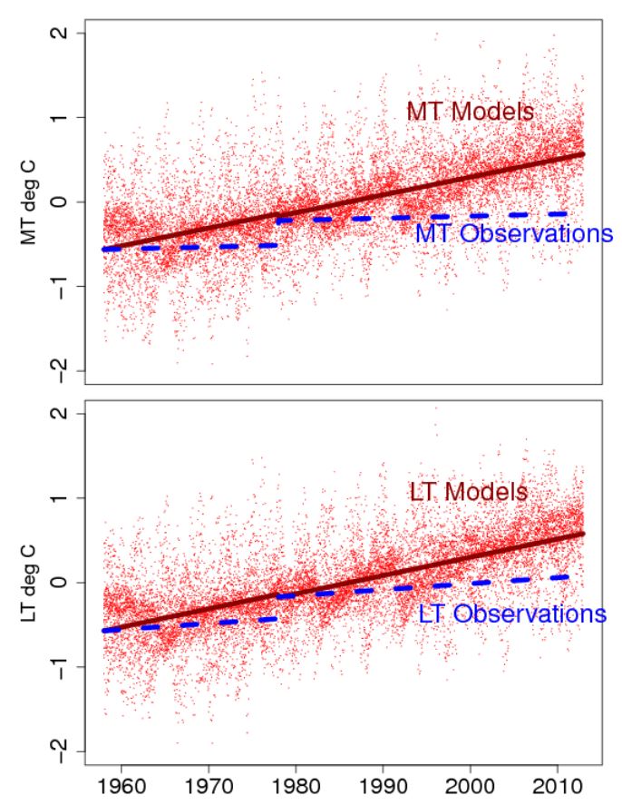
The dark red line shows the trend in the model ensemble mean. Since this displays the central tendency of climate models we can take it to be the central tendency of mainstream thinking about climate dynamics, and, in particular, how the climate responds to rising GHG forcing. The dashed blue line is the fitted trend through observations; i.e. reality. For my part, given the size and duration of the discrepancy, and the fact that the LT and MT trends are indistinguishable from zero, I do not see how the “mainstream” thinking can be correct regarding the processes governing the overall atmospheric response to rising CO2 levels. As the Thorne et al. review noted, a lack of tropospheric warming “would have fundamental and far-reaching implications for understanding of the climate system.”
Figures don’t really do justice to the clarity of our results: you need to see the numbers. Table 7 summarizes the main test scores on which our conclusions are drawn.
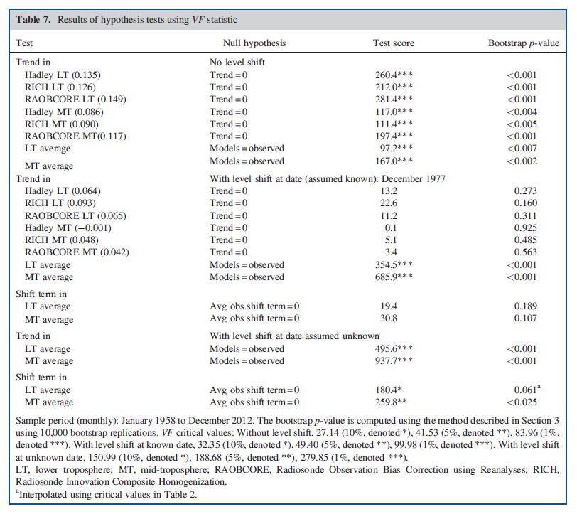
The first column indicates the data series being tested. The second column lists the null hypothesis. The third column gives the VF score, but note that this statistic follows a non-standard distribution and critical values must either be simulated or bootstrapped (as discussed in the paper). The last column gives the p-value.
The first block reports results with no level shift term included in the estimated models. The first 6 rows shows the 3 LT trends (with the trend coefficient in C/decade in brackets) followed by the 3 MT trends. The test of a zero trend strongly rejects in each case (in this case the 5% critical value is 41.53 and 1% is 83.96). The next two rows report tests of average model trend = average observed trend. These too reject, even ignoring the shift term.
The second block repeats these results with a level shift at 1977:12. Here you can see the dramatic effect of controlling for the Pacific Climate Shift. The VF scores for the zero-trend test collapse and the p-values soar; in other words the trends disappear and become practically and statistically insignificant. The model/obs trend equivalence tests strongly reject again.
The next two lines show that the shift terms are not significant in this case. This is partly because shift terms are harder to identify than trends in time series data.
The final section of the paper reports the results when we use a data-mining algorithm to identify the shift date, adjusting the critical values to take into account the search process. Again the trend equivalence tests between models and observations reject strongly, and this time the shift terms become significant or weakly significant.
We also report results model-by-model in the paper. Some GCMs do not individually reject, some always do, and for some it depends on the specification. Adding a level shift term increases the VF test scores but also increases the critical values so it doesn’t always lead to smaller p-values.
Why test the ensemble average and its distribution?
The IPCC (p. 772) says the observations should be tested against the span of the entire ensemble of model runs rather than the average. In one sense we do this: model-by-model results are listed in the paper. But we also dispute this approach since the ensemble range can be made arbitrarily wide simply by adding more runs with alternative parameterizations. Proposing a test that requires data to fall outside a range that you can make as wide as you like effectively makes your theory unfalsifiable. Also, the IPCC (and everyone else) talks about climate models as a group or as a methodological genre. But it doesn’t provide any support for the genre to observe that a single outlying GCM overlaps with the observations, while all the others tend to be far away. Climate models, like any models (including economic ones) are ultimately large, elaborate numerical hypotheses: if the world works in such a way, and if the input variables change in such-and-such a way, then the following output variables will change thus and so. To defend “models” collectively, i.e. as a related set of physical hypotheses about how the world works, requires testing a measure of their central tendency, which we take to be the ensemble mean.
In the same way James Annan dismissed the MMH2010 results, saying that it was meaningless to compare the model average to the data. His argument was that some models also reject when compared to the average model, and it makes no sense to say that models are inconsistent with models, therefore the whole test is wrong. But this is a non sequitur. Even if one or more individual models are such outliers that they reject against the model average, this does not negate the finding that the average model rejects against the observed data. If the central tendency of models is to be significantly far away from reality, the central tendency of models is wrong, period. That the only model which reliably does not reject against the data (in this case GFDL 2.1) is an outlier among GCMs only adds to the evidence that the models are systematically biased.
There’s a more subtle problem in Annan’s rhetoric, when he says “Is anyone seriously going to argue on the basis of this that the models don’t predict their own behaviour?” In saying this he glosses over the distinction between a single outlier model and “the models” as group, namely as a methodological genre. To refer to “the models” as an entity is to invoke the assumption of a shared set of hypotheses about how the climate works. Modelers often point out that GCMs are based on known physics. Presumably the laws of physics are the same for everybody, including all modelers. Some climatic processes are not resolvable from first principles and have to be represented as empirical approximations and parameterizations, hence there are differences among specific models and specific model runs. The model ensemble average (and its variance) seems to me the best way to characterize the shared, central tendency of models. To the extent a model is an outlier from the average, it is less and less representative of models in general. So the average among the models seems as good a way as any to represent their central tendency, and indeed it would be difficult to conceive of any alternative.
Bottom Line
Over the 55-years from 1958 to 2012, climate models not only significantly over-predict observed warming in the tropical troposphere, but they represent it in a fundamentally different way than is observed. Models represent the interval as a smooth upward trend with no step-change. The observations, however, assign all the warming to a single step-change in the late 1970s coinciding with a known event (the Pacific Climate Shift), and identify no significant trend before or after. In my opinion the simplest and most likely interpretation of these results is that climate models, on average, fail to replicate whatever process yielded the step-change in the late 1970s and they significantly overstate the overall atmospheric response to rising CO2 levels.


101 Comments
Reblogged this on JunkScience.com and commented:
Climate models are inconsistent with observations
Ross McKitrick writes: “The dark red line shows the trend in the model ensemble mean. Since this displays the central tendency of climate models we can take it to be the central tendency of mainstream thinking about climate dynamics, and, in particular, how the climate responds to rising GHG forcing.”
“central tendency of mainstream thinking” is an excellent portrayal. Thanks.
Regards
” it seems to me likely to be something to do with faulty parameterization of feedbacks. Also the problem persists even in studies that constrain models to observed SST levels.”
Here I looked at ERBE TOA radiation budget in relation to the effects Mt Pinatubo.
I found that earlier estimations of Lacis et al 1992 ( Hansen was a co-author ) for the scaling of AOD to W/m2 radiative forcing, based on physical analysis, were is good agreement with the ERBE data (though they were derived mainly from El Chichon observations).
However, work by essentially the same group just a few years later, reduced the earlier value of 33 to 21, thus _reducing_ the radiative forcing attributed to volcanoes.
This was done on the basis that the lower value worked better with climate models. The implied but unstated condition being: with climate models without reducing the high sensitivity of the models.
Clearly if they had followed the data, instead of effectively changing the data fit models, they would find the models needed a lower sensitivity to match the data.
The corollary of that is if they changed to model parametrisations so as to produce output that matched the data using the earlier physics based estimations of AOD forcing they would also end up with reduced sensitivity to GHG.
The predicted hotspot would melt away and fall into line with observations and the lack of warming post 2000 becomes less problematic.
Looks like CA must be aliased to WordPress, it changed by login to climategrog. To avoid confusion, it’s still me, Greg.
Thanks to Ross and Tim Vogelsang both for the post and the interesting paper. They have done novel work that deserves attention not simply for the topical issue of models vs observations, but for their development of statistical techniques for comparing trends and models. Vogelsang has done seminal work that I have long admired from a distance. It strikes me as being in the spirit of Phillips 1985, a work that we cited in our criticism of Mann’s benchmarking of RE statistics, a topic that was important in our 2005 papers, but not understood in the climate world.
Some of the earliest CA posts (2005) referred to Vogelsang’s work: see
Most red noise models used for proxy work were based on simple AR1 models, but many of the most prominent datasets seemed to be better modeled as ARMA(1,1) processes with high AR coefficients and a negative MA coefficient of about -.32.
Vogelsang (1998) reported on properties of ARMA(1,1), observing that spurious trends were particularly problematic in the red zone of high AR1 and moderately negative MA1 coeffients – exactly in the climate zone. The math of VOgelsang 1998 was slightly out of my then (and current) knowledge, but was a topic that I would have liked to pursue further.
Thanks for the kind words, Steve. Some of the best methodological work in econometrics comes about when an empirical researcher hits a snag with his/her data or needs to do something that can’t be accomplished with existing methods. My paper with Ross is a great example.
I share your view that the empirical climate literature seems unaware of statistical (or econometric) methodology that could be directly applied in many settings they face with their data. Given that climate time series have similar features to macroeconomic and finance time series, you would think empirical climate researchers would look to other literatures for well-developed approaches. During the review process for our paper, referees would request that we reference various time series methodological papers in the climate literature. When I read these papers, it was nearly always the case that the authors were trying to tackle statistical problems that had already been addressed in the econometrics literature 10 or 20 years previously. There’s a lot of low hanging statistical/econometrics methodological fruit for empirical climate researchers willing to read literatures outside of climate journals.
Now that is how a science paper should be published.
The following is a duplicate of a comment published earlier today at WattsUpWithThat.com:
The paper offers readers the results of an IPCC-style “evaluation.” In an evaluation, observed temperature time series are plotted on temperature-time coordinates together with the associated computed time series. This comparison provides for visualization of the error.
It does not, however, provide for the validation or falsification of any of the models. For this purpose, the predicted relative frequencies of the outcomes of the events must be compared to the associated observed relative frequencies. If there is a match, the model is validated; otherwise it is falsified. This comparison cannot be made because events are not a concept in the methodology of research of this kind.
Excellent review that motivates me to read in detail from this paper. I am particularly interested in the part referenced in the comment below.
“When I asked Tim if the VF method could be used in an application allowing for a suspected mean shift, he said no, it would require derivation of a new asymptotic distribution and critical values, taking into account the possibility of known or unknown break points. He agreed to take on the theoretical work and we began collaborating on the paper.”
I have not read this paper yet but I am wondering how the issue of “weather” noise is handled for the models. It can be estimated from multiple runs from the same model and only from the observed data by modeling that data, as for an example using an ARMA model, and then doing simulations.
For surface temperature series individual model runs in CMIP5 appear to show weather noise while averages show more straight line trend tendencies. Since the observed data is from a single realization of a chaotic climate it should show weather noise.
“Over the 55-years from 1958 to 2012, climate models not only significantly over-predict observed warming in the tropical troposphere, but they represent it in a fundamentally different way than is observed. Models represent the interval as a smooth upward trend with no step-change.”
GCMS will always miss a step change.
Steven, if they can’t show a step change, they are missing the physical processes which lead to that step change. Which seems to be quite fundamental to predict what will happen in the future…
Not true.
1. the can Show a step change
2. But they will always miss the timing as the timing is going to be an initial values problem.
3. it’s unclear whether capturing the magnitude and timing of step changes is fundamental to making
useful predictions about the future.
I’m unclear about 3. If the models are good representations of the future, but are just failing to pick the timing and magnitude of the step change because the initial conditions are wrong, one would expect accurate models to flat line through this period, rather than show a trend.
The fact that the models apparently reproduce a trend without the step change is problematic for prediction based on them.
Assumptions about step changes should then instead be partialed out and dealt with separately.
Seems to me the legitimate test is if models ever show the behavior or the Earth; in this case, if the ever produce a step change. My guess is that they do not, probably because they are not accurately mimicking all the important pseudo-cyclical behaviors.
30+ years after the event, with all the inputs and outputs observable, and they can’t reproduce the event. As for timing, never mind getting the year right, across a 55 year window it’s just not there, period. So it’s not that they have the mechanism right and all they lack are the initial conditions. They don’t have the mechanism right.
Suppose that’s not true, and they have the basic mechanisms right, so they got the trend right but just left out the step-change. In that case the red line would end up in 2012 below the blue line in Figure 3. Instead, it is well above the blue line, which indicates that they have an upwardly biased trend component, likely because they attribute the warming associated with whatever mechanism caused the step change to the mechanism (chiefly GHG forcing) causing the trend.
Ross McKitrick:
There is something that I don’t understand. You say that “30+ years after the event, with all the inputs and outputs observable, and they can’t reproduce the event.” How is this event described?
Given the step changes seem to have a material impact on future climates even if they are an artifact of initial conditions and weather (and are reasonably rare), useful climate models would need to model them in some shape or form. As I understand it here the argument is that the models being used as comparators were not initialised with the information sufficient to trigger the step change. Under those circumstances as I noted reliable models should not model it (nor should the average of a number of model runs show much sign of it).
To tease it out a bit further, the models may well (if they can replicate step changes) produce their own step changes that don’t occur in the obs. Multiple runs will again tend to average these out. So to really get a handle on it all you need to know the frequency of these step changes occurring (in both models and nature), and how they behave in aggregate.
Because step changes do seem to impact on future climates, but we can’t specify the initial conditions sufficiently to reproduce the historic record in the runs we are using, I suspect one needs to try and model their occurrence and impact explicitly. This at least would give some understanding of their potential impact on the future climates being predicted by the models.
However because the models seem to approximate the observed step changes (by using a trend) this suggests the step change is being modeled, even if on the above logic it shouldn’t show in the runs. It makes me a bit sceptical of the line that these step changes are simply an initial values problem, but for the sake of argument this is where that assumption leads you.
Commented without seeing Ross McKitrick’s that makes the same point much more succinctly.
Asking whether or not the models can ever generate a step change throws up another question (which has probably been asked before, but what the heck). If allowed to run on long enough, do any models ever generate an ice age? They may not be designed to project that far into the future, but their supporters always bang on about how they are based on ‘fundamental physics’ and if the physics is correct surely at some point some of them must?
Jonathan Abbott
Mr. Mosher-
Respectfully, could you lay out a bit more explicitly what you are contending is wrong with this comparison analysis of the step feature? It sounds like you are saying the models often do exhibit the prescribed step change, but often at the wrong time. However my (very basic) understanding of individual model run outputs is that the majority of them rarely ever exhibit this step behavior. Would you agree with that? If that is true we would have to assume it’s more likely there is a fundamental problem with the models than for synchronicity/out-of-phase-ness to be the reason for the discrepancy. Nothing would be PROVEN, but we would have to make that ASSUMPTION.
Note that I do understand that the ensemble mean shouldn’t be used for direct comparison to the step feature; means/averages should only be used for comparison to the trend since any steps (up or down depending on phase of various runs) would average/smooth out.
Has anyone quantified statistically how often, out of a sample of individual model runs, a similar step feature is found? And compared that to what would be expected by chance if the model outputs were just noise? Maybe it was done in this paper; I haven’t had a chance to read it.
At face value, I would say that if the majority of the model runs RARELY ever (to almost never) exhibit the behavior of the empirical data, that is as strong a signal the models have something fundamentally wrong as we are ever going to get. Apologies to the contrary make the models seem unfalsifiable.
“Mr. Mosher-
Respectfully, could you lay out a bit more explicitly what you are contending is wrong with this comparison analysis of the step feature? It sounds like you are saying the models often do exhibit the prescribed step change”
Yes the models can and do exhibit step changes so Ross isnt correct when he says they dont have “the” mechanism down. That’s an imprecise black and white description of a complex process.
The initial conditions required to get the timing correct would basically require an observation system that is far more complete than we have now.
What do I find wrong with this analysis?
Well the same thing I would find wrong with an analysis that said the climate models didnt predict the number of words in this post.
They are not designed to capture a historical step change that comes from the synchronization of psuedo periodic oceanic cycles. They cant be designed to do this.
just like they wont predict the number of words in this comment.
They WILL however produce these steps changes but the TIMING will be wrong. ie its more to do with initial conditions.
FISRT
see Ross’ comment
‘That the only model which reliably does not reject against the data (in this case GFDL 2.1) is an outlier among GCMs only adds to the evidence that the models are systematically biased.
remember that model. OK
then read this which explains how we get shifts from synchronization
Click to access GRL-Tsonis.pdf
and read the part where they see whether models can reproduce this.
Look at the model results. for GFDL !!!!
“The general mechanism observed in the actual data is observed in
both simulations. In the control run we observe three synchronization events around years
120-130, years 139-148, and years 180-188. ”
Before Folks like Ross make comments that the failure is due to “bad mechanism”
it would be wise to read the literature.
The mechanism may doubtless be imperfect but its MORE LIKELY to be an initial conditions problem
especially given the fact that the very Model Ross identifies as not being too bad actually can produce these kind of phenomena.
One problem with not spending a bunch of time reading literature.
one problem with not having reviewers who know the lit.
Mosher says:
Really? You don’t see any difference between a paper that compares climate models’ ability to replicate a major aspect of the climate over a historical interval of considerable scientific interest, versus a paper that compares climate model outputs to numbers of words in blog posts? Obtuse hardly begins to describe that comment.
Given that “the” step change in question is positive in half the models and negative in the other half, I’m not convinced they’ve got it down. As I understand your position, one model has been shown to potentially be able to reproduce synchronization breaks consistent with those identified in observational data. Even if all models could, so what? It doesn’t take away from what we found, all it does is narrow down the possible explanations slightly.
You failed to mention that we cite the Tsonis paper. There are 2 GFDL models. Yes the GFDL 2.1 model places a coupling break somewhere in the 1980-1990 decade. You’re the one arguing that modelers are unable to specify initial conditions with sufficient precision to get the timing of a break approximately correct, so you are implying that this result was a fluke. And note that Tsonis et al. analysed a control run. But also, note that in the GFDL2.1 forced series that we used, the LT and MT mean shifts terms are negative, not positive (see our Tables 5&6). The GFDL 2.0 shift terms are positive, but that’s not the model Tsonis used.
Anyway I have lost track of what your argument is, or what I’m supposedly disagreeing with. I only raised the question of step-changes in models to try and make sense of our empirical results. Are you saying there isn’t a statistically significant discrepancy between models and observations in the tropical troposphere? Because the discrepancy is there whether or not we control for a step-change.
Are you saying the models get the forcing trend correct? Because if they did, yet failed to put a PCS-sized step in the late 1970s for whatever reason, they should be producing too little warming over the 1958-2012 period, not too much. They leave out the warming associated with the PCS and yet they still produce more warming than was observed. Why do you suppose that is?
Are you arguing that there is a statistically significant warming trend in the tropical troposphere over the 1958-2012 interval? When we control for the PCS step, the trend term becomes small and insignificant in the radiosonde series. I’m not the one who first suggested this is a “potentially serious inconsistency” with models, and I’m not the one who said a lack of tropospheric warming “would have fundamental and far-reaching implications for understanding of the climate system.” Do you find nothing unexpected in the absence of warming over that long an interval in that region?
Steven Mosher Jul 28, 2014 at 1:35 PM
If I understand you correctly you are saying don’t be surprised the individual model runs don’t produce a particular step change, and further more don’t be surprised if an average of runs smooth all sign of step changes out.
All well and good.
But here’s the thing. Over time in the real world step changes occur and we want to be sure our models look through these in a way that gets their impact right on average. The predicted climate from the models needs to behave like the real world on multi-decadial time scales. If they wander off somewhere else they aren’t going to be much use.
So the question for you is how do you expect these models to behave (both individually and in aggregate) while the real world is having a particular step change?
I’m with Mosher on this, in part. I don’t think there is any expectation that models should match the timing of particular physical processes. Having said that it still seems important that outside the step change the models and obs do not match
I have a question concerning Figure 3 ….. Has the IPCC assigned its own confidence intervals to the LT and MT model ensemble mean predictions, CI’s which could be plotted as continuous lines on Figure 3 along with the plots of the central tendencies?
Individual climate model runs can show weather noise and that should result in breakpoints. It is the timing for the weather noise and the breaks that the individual climate models (and of, course the combined runs) cannot handle.
The problem is when they show approximations to break points (aka linear trends) when they shouldn’t be showing anything. It does suggest the models are gaining information on break point surrogates from somewhere other than the initial conditions (tuning? parameter estimations and assumption?)
There are two paths to root cause attribution of a phenomenon, eliminate all potential causes but one, or show that the phenomenon produces unique output that can only be explained by one cause. The former is far away for GHG warming, the latter is a depressingly short list consisting of only polar and tropospheric amplification AFAIK. Kudos to Dr. McKitrick for keeping his eye on the ball. While I lack the math chops to fully follow the arguments, I will be reading as many of the cited references that I can get for free to catch up on the tropospheric amplification debate.
“Neither weather satellites nor radiosondes (weather balloons) have detected much, if any, warming in the tropical troposphere”
There is the paper “Warming maximum in the tropical upper troposphere deduced from thermal winds” by Robert J. Allen & Steven C. Sherwood (http://www.nature.com/ngeo/journal/v1/n6/abs/ngeo208.html) that uses wind as a proxy for temperature and finds the warming: “direct temperature observations from radiosonde and satellite data have often not shown this expected trend. However, non-climatic biases have been found in such measurements. Here we apply the thermal-wind equation to wind measurements from radiosonde data, which seem to be more stable than the temperature data”
Can anyone comment on this?
Colin,
That paper was refuted the following year here:
Pielke Sr., R.A., T.N. Chase, J.R. Christy, B. Herman, and J.J. Hnilo, 2009: Assessment of temperature trends in the troposphere deduced from thermal winds. Int. J. Climatol.
not sure if this one is available on line, I made a couple unsuccessful attempts.
Thanks Matt. Here’s a link to Pielke’s blog on it:
So, if I understand this correctly, the paper is saying that the actual temps aren’t doing what they want, so they’ll use a proxy. Unless the proxy goes the wrong way, in which case they will probably revert back to the actual temps.
How Mannian of them.
McKitrick: “For readers who skip that part and wonder why it is even necessary, the answer is that in serious empirical disciplines, that’s what you are expected to do to establish the validity of novel statistical tools before applying them and drawing inferences.” I myself always appreciate Dr. McKitrick’s writing, and especially so in this quote. Yes, it is transparently obvious that his prescription is what one in fact MUST do in “serious empirical disciplines”. I feel sad that some who ascribe to themselves a great love of climate science do not treat their field as a serious empirical discipline in this way.
William – I was going to quote that paragraph as well – I laughed out loud when I read it.
One of the more enjoyable blog discussions that ever occurred happened a couple of years ago on Bart Verheggen’s site. Commenter VS took on a good part of the climate community in a marathon discussion. My guess was VS is Tim Vogelsong.
I am not VS.
Can we call you VS for short? Or TS?
Re: Tim Vogelsang (Jul 25 10:06),
Sorry for the surmise, Tim. VS was mathematically gifted, and a econometrician with state-of-the art mastery of times series.
That discussion is worth going back to if you want to understand that the published confidence interval for climate predictions are consistently too narrow for systems such as the climate with a (near) unit root. There was a high probability for the climate to leave the bounds. No surprise that it is doing so.
How about a link?
If you look at that thread, you’ll see that VS can write in (fluent) Dutch.
Is the 1977 step change real, or is it just a bad transistor in the radiosonde receiver?
The Pacific Climate Shift was first identified in the fisheries literature when major shifts in locations of tuna and anchovy harvests (IIRC) started to be noted around 1980. As the years went on people noted step changes in numerous parameters around the Pacific rim, such as the FANB record in Alaska: see http://climate.gi.alaska.edu/Bowling/FANB.html. Tsonis et al have published several studies looking at step-changes in the climate system as chaotic bifurcations.
in fact Tsonis 2007 argues that the sychronization and regime shift is captured by GFDL
Steven Mosher
Posted Jul 24, 2014 at 5:24 PM | Permalink | Reply
Not true.
1. the can Show a step change
Steven, this sounds like the “they can and produce 15 yr pauses” but not when they are observed. That means to me that they are useless models.
McKitrick: “As for timing, never mind getting the year right, across a 55 year window it’s just not there, period.”
Are we sure the ‘step change’ does not show up in the models? My understanding would be that results of individual models (i.e., GFDL 2.0, for instance) are still reported as ensembles. As such, realizations of a particular model would (if we accept the timing of a step change would be an initial value issue) show the step at different times throughout the period. Seems the ensemble for ‘that’ model would be a sloped line (i.e., averaging out all the step changes from the individual realizations). The final full model average (i.e., as shown in the Figure 3 panels), would average the results even more. Assuming the ‘initial value’ issue is accurate and that individual model’s realizations could indeed get a ‘step change’ in MT/LT temps, then I see no reason why anyone would expect the step change to show up in an average of the (averaged) model ensembles.
Think of it this way. The models all exhibit positive trends, in all cases but one statistically significant. None of the models yield a significant mean shift, and half are + and half -. So in terms of what the models are programmed to do, it’s a safe bet that they are programmed to mimic a physical process that yields an upward trend, but not programmed to mimic a physical process that yields step changes, bifurcations, etc. If the representation of the trend component were unbiased, the models would yield a flat line that runs parallel to the blue line but doesn’t jump at the 1979 step. Instead the models yield a trend biased significantly high. If you look closely at Figure 3 you can see that the blue and red lines meet at the top of the step change, as if the size of the step was the exact measure of the average trend bias in the models.
“Instead the models yield a trend biased significantly high. If you look closely at Figure 3 you can see that the blue and red lines meet at the top of the step change, as if the size of the step was the exact measure of the average trend bias in the models.”
I guess I see your point (the actual physics are not captured). However, I would think this criticism will be rather easily dismissed. We are but one (or maybe 2 for the MT) real world ‘step changes’ away from being in general accord. I don’t think there are claims that the models capture these types of emergent phenomena yet (i.e. an abrupt step change (maybe due to some sort of physical regime change) vs. longer term “average” changes)…or are there such claims?
More importantly, should have mentioned that I really enjoy the ‘Spirits Bright’ CD. 😉
Hey, thanks!
Thanks for that Ross.
Can the models capture any kind of a phase change not directly coded into them? I’m thinking of threshold functions similar to neuronal activation. These are not initial value problems in my mind. It seems to me that any damped, driven dynamic system will have ’emergent’ behaviors of some kind.
S. Geiger Jul 25, 2014 at 11:21 AM
“We are but one (or maybe 2 for the MT) real world ‘step changes’ away from being in general accord.”
The problem is that given the behaviour being discussed here the models will show a further trend response when the real world ‘step changes’ occurs moving them increasingly ahead (assuming upward step changes).
For this argument to work I think you need to assume models in aggregate smooth out the step changes (perhaps not unreasonable), but something in the climate is causing a bias to upward step changes that the models do pick up.
However if this were the case the trend result should be smoothed over the complete time period between step changes, not much more acute as appears to be shown here.
Ross said “Think of it this way. The models all exhibit positive trends…”
That sentence is all of it.
Complexity (the reality, the molecules of matter of the atmosphere and oceans) can’t yet be modeled.
Steve; this comment is coat-racked onto a technical article. Please avoid generalized complaining.
Terry,
Complexity theory is the logical understanding of a complex system.
Abstraction of some detail of a complex system only gives you an abstract simplification of that detail.
Global Average Temperature is a very abstract simplification of the global climate state.
Does anyone think that global temperature over time is an understanding of the climate history?
jim z:
Thanks for giving me the opportunity to clarify. In addition to providing a simplified description abstraction increases statistical significance. Thus, for example, the more abstract description “male OR female” references no fewer humans than the less abstract description “male” and may reference more humans. If it contains more then the sample size is increased with consequential increase in the statistical significance of the conclusions.
Abstraction is one of the ideas that lead to thermodynamics. The “macrostate” of thermodynamics is an abstraction from the associated system’s “microstates.” This idea seems, however, to be misunderstood by many climatologists.
If there are step changes, just how does linearly increasing CO2 cause that? It causes everything I guess.
There are quite a few comments lamenting inability to model step changes, but Mosh is right that the significance is unclear (this takes nothing away from Dr. McKitrick’s analysis). If your car is climbing a hill and the transmission downshifts, the rpm will make a step change. But if your model is just supposed to predict the speed of the car, capturing the step change in rpm adds nothing. Climate models don’t necessarily need to capture local step changes caused by ocean current migration as long as basic poleward heat flow is adequately modeled.
In your example there’s a fixed mechanical connection between RPM and wheel speed. Suppose you don’t know it and you are constructing a regression model to estimate it. Your model is of the form (Speed) = a + b(RPM). You ride in a car with 2 speeds and collect data on speed and RPM as you go up a hill, but you ignore the gear change. Obviously the line you fit will yield a biased value for b.
Now suppose you are tweaking a climate model to warm up X degrees over an interval where CO2 rose Y%, and you ignore the step change along the way. Again, you will wind up with a biased model because you will attribute the portion associated with the step change to the CO2 increase. I’m not suggesting the process of fiddling the knobs on a GCM is that simplistic, but that would explain the mismatch we found.
I see what you are saying about fitting the linear regression, I guess my analogy fell short. AFAIK all GCMs are “control volume” in engineering lingo, very roughly
(heat input) – (heat loss) = delta T
If something inside the controlled volume has capacitance, it might slowly store heat, and then rapidly release that heat in a cyclical fashion, and each release will look like a step change in the T data. That won’t introduce any error in the controlled volume equation though as long as you have enough data in the time domain. The way to follow the control volume equation is to draw a straight line through the step changes, because in the end the capacitance won’t change the trajectory. What am I missing?
You are describing a brick in an oven that acts nothing like a brick. What you are missing is the mechanism that explains why your brick stays cool for an hour then suddenly gets hot. Capacitance won’t get you that. You need a mechanism, like an air conditioner inside the oven blowing on the brick until the oven melts the power line. Once you postulate a mechanism, then you need to see if the data are consistent with it. And that’s what we tested.
Or to put it another way, thermodynamics rules out behavior like an automatic transmission. There’s more to this than mathematical abstraction. It has to be physical.
Analogies help me but they are not helping me here. Dr. McKitrick wrote:
“[The Pacific Climate Shift in the late 1970s] is a well-documented phenomenon (see ample references in the paper) in which a major reorganization of ocean currents induced a step-change in a lot of temperature series around the Pacific rim.”
If solar insolation if flat throughout, how can that be anything but a manifestation of capacitance? You can go to SkS or RC and find some “just so” stories about how the pause is caused by sequestration of heat in the oceans. It is not my argument but I cannot refute it. If it is true that heat can pass through the atmosphere, be stored in the oceans, and later manifest as a step change in atmospheric temperature due to a change in ocean currents, then this can be considered capacitance. A control volume equation need not consider intermittent capacitance to show the correct trend over long intervals. So the mechanism you are asking me for is whatever mechanism you are invoking when you say that a change in ocean currents caused a step change in temperature. Specifically, what mechanism are you invoking for the Pacific Climate Shift in the statement I quoted above, and how can it be differentiated from the engineering concept of capacitance?
To be clear, I agree with a claim that if a GCM cannot model a decadal scale step change such as the PCS, it is unlikely to have skill in forecasting climate on a decadal scale. I don’t think this is a major concern regarding the ability of a GCM to forecast runaway heat (those problems lie elsewhere). On the other hand, tropospheric amplification – based upon first principles in physics – is primary evidence about AGW for the reasons outlined in my first comment.
Not being an expert in the underlying physics I am loathe to try and postulate how a reorganization of ocean currents could manifest as a rise in the average temperature without it necessarily involving release of heat previously stored, so take the following with appropriate caveats. First, energy is not equivalent to temperature. In the analogy I gave, the brick heats up suddenly, even though the total amount of energy used by the system drops (because the AC unit shuts off). In a system as complex as the climate I have no difficulty imagining that there are circumstances in which, following a reorganization of ocean currents, the same amount of energy is distributed in such a way that the average over the tropical air temperature field steps up (or down). Willis points toward one such mechanism in his comment below. All you really need is to allow one or two parameters normally assumed to be invariant in a model to change in response to changes in other parameters, such as allowing the lapse rate to vary or cloud formation processes to vary, and there should be no difficulty coming up with any number of possible mechanisms that exhibit discontinuities.
Second, if the step change is merely a release of stored-up heat, the point of my analogy was that your model can’t resemble a brick because bricks don’t work that way. You need a more complex mechanism that explains storage and periodic release of heat on some deterministic timetable. GCMs don’t seem to generate step-changes, even to match the historical record, so it looks like they are “brick” models, so to speak.
Third, if capacitance/discharge really is the story, you still need to ascertain at what point in time the heat began to get stored; you can’t assume the time window coincides with the time window of the rise in CO2 forcings. The curious match between the red line and the size of the step change over the 1958-1978 interval suggests to me that such an assumption is being made. But if, for instance, the PCS event released heat stored over a millennium, and the models attributed that rise to the effects of GHG emissions since the 1950s, then there will obviously be a bias in the representation of the forcing mechanism in the model.
OK, I think we hammered out some agreement. When you wrote:
“Now suppose you are tweaking a climate model to warm up X degrees over an interval where CO2 rose Y%, and you ignore the step change along the way. Again, you will wind up with a biased model because you will attribute the portion associated with the step change to the CO2 increase.”
This is true if, and only if, the intializing assumption of equilibrium in the control volume equation is false. It would be false if heat had been sequestered in the oceans for a millenium.
Dear Dr. McKitrick:
A car’s transmission is a putative analogy to the climate via the formula (Speed) = a + b(RPM) for a transmission. In the development of this analogy, the change in the global equilibrium temperature at Earth’s surface substitutes for the speed of the car and the change in the logarithm of the CO2 concentration substitutes for the RPM of the car’s engine.
However, there is a pitfall enroute to this analogy. This is that the speed is an observable feature of the real world but the change in the equilibrium temperature is not. In consequence, the RPM provides perfect information about the speed but the change in the logarithm of the CO2 concentration provides no information about the change in the equilibrium temperature. This conclusion follows from the definition in information theory of the “mutual information” as the information theoretic measure of the intersection between observable state-spaces.
The mutual information is the information that is available for the control of the associated system. In the relation between the change in the logarithm of the CO2 concentration and the change in the equilibrium temperature, the mutual information is nil. Thus the controllability of the equilibrium temperature that is evident to the makers of governmental policy on CO2 emissions is illusory.
Misunderstanding of the important difference between the climate and a car’s transmission is leading the people of the world into a public policy disaster. As I strive to avert this disaster I need your help if you are able to provide it.
Ross, Excellent work; congratulations to you and Tim Vogelsang on the paper. And thank you for a very clear article. It would be great if you could also post the results applying to CMIP5 models at CA, when they become available.
When you analyse the CMIP5 models, might you also look at trends over the period 1979-2013, with no shift allowed for, thus updating your previous analysis of the satellite era? Although it is a shorter period, I suspect the results will be fairly similar to those for the full period with a break allowed. And the extra data sets and avoidance of the break issue may make the results seem more robust to some climate scientists.
No doubt you are aware that Figure 9.9 in AR5 WG1 shows that the average model trend over 1988–2012 in tropical (20°S to 20°N) lower tropospheric temperature over the oceans was 3x that of the satellite observations and the best reanalysis dataset (ERA-interim).
If you are modeling the residuals of a series with step changes those residuals and thus the model will change between ignoring the step change and accounting for it.
As an aside I think the overall trend will be different depending whether you account for or ignore the step changes, i.e. assuming one linear trend versus segmented linear trends.
I did a breakpoint analysis of the 149 climate model runs for the historical series for the global surface from 1964-2005 using the strucchange library in R and the breakpoints function. The series were all used as monthly. I did 2 analysis. For the first the h parameter was set at 0.15 (meaning a maximum of 6 breakpoints) and with breaks set at 2 (or a maximum of 2 breakpoints) for the second.
In the first analysis all the individual climate model runs had at least 2 breaks and maximum of 5 breaks with most having between 3 and 4. In the second analysis all runs had 2 breakpoints with the first occurring on average around 1982 and the second on average around 1993. The scatter around the averages was broad and particularly so for 1982. If nothing else the analysis shows that the individual climate model runs for surface temperature have some structure.
I believe the paper being discussed on this thread deals with the lower and mid troposphere temperatures and my analysis was for surface temperatures. I would be surprised if the climate model individual runs for the troposphere had a much different structure than the surface but I could check a few. KNMI is a great source for this data.
Kenneth, the R breakpoints routine assumes independent error terms, so it’s not robust to autocorrelation. There are methods in the literature that apply in the AR1 case — see our lit review. Our method is robust to higher-order autocorrelation. Still, it sounds like you detected breaks the major volcanoes, which are programmed into the models.
Thanks for the comments Nic. I hadn’t really studied Figure 9.9 before, but there I see two important features in it. As you note, the average model temperature trend is about 3x the average observed trend, which is why I assume the CMIP5 versions of our results will be much like the CMIP3 versions.
The other interesting point is that the observed temperature trends are almost invariant to the observed H2O trends, whereas in the GCMs the two move in lockstep. This is another trend comparison crying out to be examined! They don’t put a trend through the observational points (admittedly there are only 5, but we could exploit the time series dimension to deal with that). So it looks at a quick glance like the observations fall on the same line as the models, but that’s because there’s only one line in the chart. But just compare UAH to ERA-Interim to get the sense of the invariance issue.
The 5 observed H2O trends vary over 0.1 to 1.4%/decade, and temperature trends over that range only increase from 0.08 to 0.14 C/decade, a span of 0.06. The same vertical range of modeled H2O trends implies an increase in temperature trends of 0.2 C, about 3x larger.
If the feedback process takes a change in the water vapour trend and yields a change in the temperature trend, that chart implies the observed feedback strength is 3x stronger in the models than in the observations.
Ross, your point is well taken. I would guess that autocorrelation can screw up the information criteria evaluation. It is time for me to read your paper. My point remains though that for CMIP5 individual model surface historical temperature series I can see visual structure that appears as step changes.
I need also to look at the tropics area which is the focus of the paper under discussion. I have been looking at global data. I have started to read the paper and saw what I was going to suggest about applying this breakpoint method to the algorithms used to adjust station temperature series. It was a bit off putting to see that the method deals with single breakpoints and likes to know that one exists.
Kenneth Fritsch Posted Jul 25, 2014 at 3:32 PM
Thanks for that, Kenneth. I and others have shown that the global temperature output of GCMs is merely a linear lagged transformation of the input. As a result, they show step changes for e.g. volcanoes, and in many cases show variations from the ~11-year cycle of solar forcing.
However, such changes from the volcanoes and from the sunspot cycle are NOT present in the observational record, and thus appear to be spurious effects of the linear nature of the models.
Finally, Ross and Tim, very nice work, well cited, and well explained. My congratulations.
Best regards,
w.
Compliments on key statistical insights.
This is an excellent example of Einstein’s Razor
Traditional concepts of accuracy and precision are typically ignored or treated wrongly in exercises such as CMIP. One of my earliest posts was about the need to include all runs from a given model – even those rejected by the modellers – in the estimation of error bounds. You cannot set proper error bounds if you preselect which outcomes are going into the error estimation and which ones are not. Then, there is a problem with taking an average between modellers, as is commonly done. The resulting ‘average’ suffers because not all prior model runs are included in the average. There are some which are excluded on justifiable grounds when a proper error is found, but if runs are excluded from an average because the modeller did not like the look of the outcome, that it not scientific.
There are reasons to be cautious about the results of some runs. Here is an example from Australia’s CSIRO as reported in Douglass, D.H., J.R. Christy, B.D. Pearson, and S.F. Singer, 2007: A comparison of tropical temperature trends with model predictions. International Journal of Climatology, 27: doi:10.1002/joc.1651, table II(a). The left column shows barometric altitude in hPa, the middle columns shows the temperatures modelled by CSIRO Mark 3, expressed as millidegrees C per decade and the right column the ‘average’ of 22 GCMs for CMIP3.
Surface 163 156
1000 213 198
925 174 166
850 181 177
700 199 191
600 204 203
500 226 227
400 271 272
300 307 314
250 299 320
200 255 307
150 166 268
100 53 78
Those used to working with numbers might raise an eyebrow at the closeness of temperatures, modelled versus average, at 600, 500 and 400 hPa. More eyebrow exercises might follow from the claim of trends of 1 thousandth of a degree per decade inherent in this overuse of significant figures. One wonders about the amount of cross-comparison done before the final preferred model run is submitted.
As a generality, modellers tend to calculate statistical precision while downplaying the importance of accuracy. It is not ok to report temperatures to a thousandth of a degree when the instruments are incapable of that performance. There is abundant literature about measurement problems (accuracy errors) in balloons and sondes, as Ross McKitrick and Tim Vogelsang note. Ditto for ocean temperatures, TOA satellite radiation balances, ocean pH, etc etc. New generations of instruments so often show accuracy errors in what was formerly thought to be the best of instruments. No amount of dense sampling can overcome such accuracy errors, though precision should be improved.
Geoff, you highlight the systemic failure to report Type B uncertainties and ignorance of BIPM JCGM 100:2008 Evaluation of measurement
data — Guide to the expression of uncertainty in measurement
If I remember correctly, there is an annual (seasonal) rise and fall in surface temperature (partially driven by the eccentricity of the earth’s orbit (which is removed by converting to anomalies). This annual rise and fall in temperature in the tropics is amplified in the upper atmosphere as expected from models (at least according to a Santer 2005? paper that deserves more scrutiny). So we are stuck with a dilemma: Seasonal warming is transmitted to the upper atmosphere with amplification by a well-mixed, turbulent atmosphere, but decadal warming clearly has not been. Yet decadal warming is the net result produced by decades of seasonal warming and cooling.
Although I am convinced that the best data we have shows a discrepancy between models and observations over decades, data on seasonal changes should be innately more reliable. I’d like to see the seasonal and decadal amplification of warming analyzed side-by-side to see which is more robust. Did Santer analyze all of the seasonal data or just part of it?
More than twenty years ago, after three years of analysis a working party established to validate a widely used stochastic model agreed with one of its members, Professor R S Clarkson, who observed that a model which did not allow for step changes, be they positive or negative, which were known to have occurred and which would continue to occur, was not a very useful tool for prediction purposes. When Clarkson’s thesis was proved by the outcome, Professor A D Wilkie updated his model, which is now far more realistic, but can still occasionally fail spectacularly to provide accurate forecasts.
http://www.jstor.org/stable/41141063
And investment models are dependent on far fewer variables than are climate models.
Here is high resolution evidence for a step change in the climate state in the southwestern Pacific in 1893 (from one which had apparently lasted at least 244 years):
Sea surface temperature variability in the
southwest tropical Pacific since AD 1649
K. L. DeLong
T. M. Quinn
F. W. Taylor
Ke Lin & Chuan-Chou Shen
NATURE CLIMATE CHANGE VOL 2
NOVEMBER 2012
A prime focus of research is differentiating the contributions
of natural climate variability from those that are anthropogeni-
cally forced, especially as it relates to climate prediction
1–3. The short length of instrumental records, particularly from the
South Pacific, hampers this research, specifically for investi-
gations of decadal to centennial scale variability1,4. Here we
present a sea surface temperature (SST) reconstruction de-
rived from highly reproducible records of strontium-to-calcium
ratios (Sr/Ca) in corals from New Caledonia to investigate
natural SST variability in the southwest tropical Pacific from
AD 1649–1999. Our results reveal periods of warmer and
colder temperatures of the order of decades during the Little
Ice Age that do not correspond to long-term variations in
solar irradiance or the 11-year sunspot cycle. We suggest that
solar variability does not explain decadal to centennial scale
SST variability in reconstructions from the southwest tropical
Pacific. Our SST reconstruction covaries with the Southern
Hemisphere Pacific decadal oscillation5 and the South Pacific
decadal oscillation6, from which SST anomalies in the south-
west Pacific are linked to precipitation anomalies in the western
tropical Pacific6. We find that decadal scale SST variability has
changed in strength and periodicity after 1893, suggesting a
shift in natural variability for this location.
Matt Skaggs says: Posted Jul 27, 2014 at 9:03 AM
Matt, while I agree with you that the step change can be considered a capacitance, it is both more, less and different than a capacitance.
There is a periodic change in the Pacific ocean currents which leads to a step change in the temperature. What changes is the rate at which the excess heat can be moved from the tropics to the poles. In one phase of the PDO, the movement is enhanced, and in one phase, the movement is hindered. Of course, this causes a change in the global temperature.
However, this does not necessarily imply that there is some large amount of heat being stored and later released in a capacitative manner. The increase in global temperature perforce increases radiative losses, parasitic losses, and losses due to emergent phenomena (primarily tropical cumulus and buoyancy-driven thunderstorms). As a result, while we can postulate greater heat storage, there is no need to invoke it in order to explain the shift in temperature.
Finally, the changes in the PDO are temperature driven—when the globe is cooler, the PDO shifts to the mode where it inhibits the tropical-to-polar heat flow, and vice versa.
The problem that Dr. McKitrick is pointing to is that the models do not model this emergent, active behavior of the PDO, and that as a result, drawing a straight line from beginning to end ignores the responsive nature of the climate … and that means that the models are getting the right answer, but for the wrong reasons. In addition, they will only get the right answer during the warming phase of the PDO. As they are entirely forcing driven, during the cooling phase of the PDO, they will be way off the mark.
Let me cite the inability of the models to simulate the current “pause” following the recent phase change of the PDO from warming to cooling as an example of this error at work …
w.
Willis,
I don’t disagree with anything you wrote, but this sentence still has me wondering whether you are missing the point:
“…the models do not model this emergent, active behavior of the PDO, and that as a result, drawing a straight line from beginning to end ignores the responsive nature of the climate.”
I agree, and I have no problem with your ideas about emergent phenomena and the potential role of tropical storms, but a clear distinction needs to be made. If you are modeling decadal temperature changes, you cannot ignore “the responsive nature of the climate.” I think we can agree that the step is either capacitance or something else (you described “radiative losses, parasitic losses, and losses due to emergent phenomena, but the step was up, gains are harder to visualize). If it is caused by capacitance (and the equilibrium assumption at initialization is correct, see my most recent comment above), the best approach is to draw a straight line through the step. If it is instead something else, it should appear as a change in the “heat input” or “heat loss” term of the control volume equation. If the “something else” is correctly modeled in magnitude but not tempo (i.e. misses the step), you will still want to draw a straight line through it. If the magnitude is off, the step is irrelevant, the model is wrong. So it still works out that if the control volume model has the magnitudes right, and there was no stored heat unaccounted for at initialization, then the correct way to determine long term trend is to draw a line through the short term fluctuations. This is exactly why you would choose a control volume equation, because you cannot be sure what happens inside the box, but you have a good grasp on what goes in and out. (And just as a disclaimer, I don’t think the models get magnitudes right and the entire control volume equation has layers of uncertainty.)
Ross,
would you like to comment on Gavin Schmidt at RC:
The new econometric techniques described seem interesting, but the application to climate models is silly. The idea is that one can look for trends including jumps and do the comparison between observations and models. The problem is that the ‘jump’ identified is the ‘Pacific Climate shift’ sometime around 1976, is very clearly an expression of internal variability of the climate system (like ENSO, or the NAO). In comparing that to the models, you would need to be looking at the internal variability there too, but McKitrick instead uses the ensemble means to do the comparison. These only defines the externally forced part of the variability, and so he is guaranteeing that he will not find a match. Conceivably if the shift in 1976 was externally forced (and I’m not aware of any evidence that it is), you would expect to find a match with models only if there were that forcing applied, but since we don’t know of any such forcing, that is obviously not included in the GCMs, and so a mismatch is again guaranteed. An interesting study could have been done, looking at individual simulations, on how often events like the shift occur in the models (which might reveal deficiencies, or not), but to use these internal shifts as an argument that overall sensitivity is too high is, as I said above, silly. – gavin]
10 of the models we looked at contributed only single runs (Nos. 3,4,5,6,7,8,13,14,15,16,22,23), so if Gavin is correct, in the model-by-model results, those ones should come out better. Yet half of those 10 single runs yielded negative step-changes, ie they get the sign wrong. So the problem is not just averaging. If the models got the forced component right and only lacked the internal variability (step change) they’d project less warming than was observed over the interval. But instead they project significantly more warming. Also, the models would yield insignificant trends over the interval, as do the observations. Gavin has likely not read the paper nor given any real thought to the results.
Here’s a more detailed reply.
There is a well-established literature making these kinds of comparisons. We have just refined the methods and carried out an application on an area of considerable current interest in the literature. Waiving it away as “silly” sounds dismissive and defensive.
It is very helpful that Gavin affirms that the PCS is a manifestation of internal variability! One of our referees argued that maybe the jump is a manifestation of the forcing, in which case we shouldn’t control for it. We argued back (and stated in the paper) that we assume the jump and the trend are two fundamentally different processes and the researcher wants to control for each separately. Gavin is here saying the same thing: the jump is an internal process, the trend is external forcing. That’s why it is important to control for them separately in order to make a proper comparison of the trends.
We report results for the overall weighted-mean GCM but we also report results model-by-model, and 10 of the models only provide a single run. Yet the pattern of failing to reproduce the step-change is the same in those single runs as it is for all the models together. So averaging isn’t the issue, since the pattern isn’t there in individual runs to begin with.
Pay close attention here. Gavin’s point is valid but it proves the opposite of what he alleges. If the models got the forcing (i.e. the trend) accurately, and only left out the internal variability (i.e. the PCS jump), they would project less warming than was observed. In that sense the ‘guaranteed mismatch’ should have been that models produce too little warming. Yet they projected too much warming, and the discrepancy is statistically significant. And the trend mismatch becomes more significant, not less, when we control for the mean shift in the observations, the opposite of what Gavin’s argument implies.
It is a straw man to say we “use these internal shifts as an argument that overall sensitivity is too high”. What we show is that, when we control for the PCS, namely the “expression of internal variability of the climate system”, we end up with trends in the LT and MT that are very small and statistically insignificant. If the models were getting the forcing right over the 1958-2012 interval they too would yield small and insignificant trends. But, other than GFDL, they yield relatively large and significant trends. The prima facie meaning of this finding is that the forcing response is generally too high in the models. For Gavin to dismiss this all as “silly” is, to say the least, inadequate, especially when his own supposed counter-argument actually supports the over-sensitivity interpretation.
Ross McKitrick:
Climate sensitivity analysis has a shortcoming. The equation that incorporates the equilibrium climate sensitivity as its proportionality constant conveys no information to a policy maker about the outcomes from his or her policy decisions. In the absence of this information, the climate remains uncontrollable after decades of research and the expenditure of hundreds of billions of dollars. Making matters worse, certain policy makers have proceeded to make policy on the assumption that they have information when they have none.
In view of the worthlessness of the equilibrium climate sensitivity as a concept supporting policy making, I propose abandonment of it in favor of an approach that provides a policy maker with as much information about the outcomes of events as possible. The starting point would be to identify these events.
I don’t have much to add to Ross’ point by point response. At the end of the day, we are doing the same sort of empirical trend comparison analysis as was done by Santer et al (2008) (see our references). The differences between what we do and what Santer et al (2008) do are:
1. We look at a longer time period (1958-2012) than Santer et al (1979-1999).
2. Because our time period spans the Pacific Climate Shift, we control for the PCS by including a level shift dummy variable to the empirical specification.
3. We use more modern methods for inference about trend parameters that are robust to fairly general forms of serial correlation in the data.
If our analysis is “silly”, then so is the analysis of Santer et al (2008). They compare individual model runs to observed temperature data (as we do). They also compare model ensembles (averages) to observed temperature data (see their Section 4.2) (as we do). Unlike Ross, I won’t speculate as to whether Gavin has carefully read our paper or not. However, I will speculate that Gavin has carefully read Santer et al (2008) with all of its ‘silly’ analysis because Gavin is one of the coauthors.
One important thing to keep in mind about the analysis in Santer et al (2008) from a statistics/econometrics perspective, is that while they correctly point out that earlier analysis by Douglass et al (2007) fails to use inference procedures that are robust to serial correlation (a big no-no when analyzing temperature data), Santer et al (2008) implement a test based on a very old approach based on some ideas in a paper by the famous statistician, Bartlett, back in 1935*. While Bartlett’s ideas showed deep insights at that time, the statistics and econometrics literatures have made many important advances in robust inference since then. The Bartlett approach amounts to a degrees of freedom correction for a t-statistic that is only valid if the serial correlation is of AR(1) form. Moreover, when the serial correlation becomes very strong and the sample size is not large (relatively speaking), Bartlett’s approach can have serious computation issues (like a negative effective sample size). I’ve run some Monte Carlo simulations using the Bartlett approach and it can go haywire when serial correlation is strong even if it is AR(1). If the serial correlation is different from AR(1), then Bartlett’s approach is invalid and can give misleading inference in general.
You would think that serious empirical researchers in the climate literature would seek the most current and best statistical tools to analyze their data rather than rely on a 79 year old method that is, from the modern perspective, too simplistic for the job at hand. Now who is being ‘silly’?
Gavin’s comments at Real Climate sometime back on the Santer paper, and in particularly about using climate model trend averages, has a personal point of interest for me. I read Gavin’s arguments against using model averages and se’s to make observed to model comparisons and knowing he was a coauthor of the paper on my first read of the paper I misinterpreted/misread the equation where the authors did indeed make the comparison Gavin opposed. Lucia quickly straightened me out (in no uncertain terms) and as a result I could only conclude that Gavin did not understand what was done in the paper. I do not know if others picked up on this but because of my misreading it has stuck with me.
As a matter of satisfying my curiosity about the surface temperatures in the tropics (20S-20N) I did some rather unsophisticated analyses of the 3 observed and 42 CMIP5 climate modeled RCP45 series from 1958-2012. I did breakpoints using the now suspect breakpoints function in R. I estimated segmented and whole series trends and used the resulting residuals to determine the best fitting ARMA model. Finally I estimated adjustments of the CIs for trends based on ARMA model simulations.
As an aside I have found on further investigation that the strucchange package from R with the breakpoints function (that I have used here) requires the sandwich package which in turn deals with HAC as described in the link below. I have not gone through the breakpoints function in detail to determine how HAC is handled nor am in a position to judge how well it might handle HAC.
Click to access sandwich.pdf
Using a maximum of a single breakpoint the Pacific Climate Change is displayed in the observed series (HadCru, GISS and GHCN) at August 1976. The modeled series under the same conditions all showed a breakpoint but at random dates throughout the series and even avoiding the 1977 time period. I think the models are not expected to time or are capable of timing weather and/or climate change events and particularly so when the initial conditions are not controlled.
The trends, whether calculated for the entire observed or modeled series or with the segmented parts of the series, all were estimated to be significant but without the adjustments for autocorrelation. In order to obtain an estimate of the adjustments required I fit the model and observed regression residual series to an ARMA model by first looking at the alternatives of (0,0), (1,0), (2,0), (1,1), (0,1) and (0,2). With these choices of ARMA models, the calculated Box test p.values with lags to 60 months indicated that these models did not reduce the autocorrelations to satisfy independence. These ARMA models all had large positive ar1 values approaching unit roots. In order to satisfy a Box test p.value of 0.30 and avoid approaching within the confidence intervals of a unit root I used higher order ar ARMA models. Using that ARMA modeling approach I continued not to satisfy the Box test and ar1 criteria for a couple of the CMIP5 models and the GISS series for the observed.
A 10000 replication simulation of a typical ARMA model (with higher order ar) for the observed and model series resulted in a required adjustment based on the 95% confidence intervals over those with white noise as follows: For white noise only of approximately +/-0.004 degrees C per decade and for red and white noise for models of approximately +/- 0.030 and for observed series of approximately of 0.061 degrees C per decade. The surface trends (mean= 0.146, sd=0.03, se=0.005) for most of the climate models with these adjustments remain very significant while the observed series are significant but less so (mean=0.106 degrees C per decade).
Using the Breusch-Pagan test for heteroskedasticity on the model and observed regression residuals rejected 27 of 42 climate models for homoskedasticity and none of the 3 observed series.
How these crude analyses of surface temperatures relate to the work of the paper being discussed here in any detail is not necessarily apparent, but nothing found contradicts the findings in the troposphere. What was surprising for me was how close the model and observed series autocorrelations approached unit roots. I was aware of high autocorrelations with monthly temperature series from previous analysis but not this high. If my calculations are correct I can see where perhaps the more traditional methods of breakpoint and trend analyses might fail.
I have often wondered if the appropriate stand on comparing observed temperature series with those from climate models is one of waiting until the models are ready for prime time.
The breakpoint dates 95% confidence intervals for the 3 observed series were July 1976 to May 1978 for HadCru, July 1976 to June 1979 for GISS and July 1976 to July 1979 for GHCN. The breakpoint dates for the modeled series were, as noted previously, randomly spaced over the 1958-2012 time period, but the 95% CIs for dates were narrower than the observed and varied from 0.5 years to 2 years.
Here is my last post on my exercise comparing 42 CMIP5 RCP45 model runs for mean temperatures 1958-2012 for the zone 20S-20N with the observed counter parts using HadCru, GISS and GHCN. I used annual averages after obtaining from monthly data very high ar coefficients that approached unit roots and some models with heteroskedasticity. Breakpoint determination was a problem due to HAC and the resulting dating uncertainty. It appears that using annual data overcomes all these deficiencies.
What surprised me was that using annual data regression residuals results in excellent ARMA model fits of (2,1) and (1,1) and further that the ar coefficient was often negative. An ARMA model with a negative ar coefficient can have a decreased CI range for trends from what the range would be for the same model (same standard deviation) with white noise only. The standard deviation for the ARMA model with negative autocorrelations while having a lower trend CI range than its white noise only counterpart will have an increased standard deviation over the white noise only counterpart.
In the comparison of the mean trend of the 42 model runs to the mean of the observed series, we have a modeled mean of 0.146 degrees C per decade and an observed mean of 0.106 for the period 1958-2012 and the zone 20S-20N. The standard error of the modeled means is 0.005 which in my view means that the observed trends are less than those of the models by a statistically significant amount. What makes a comparison of this type better is that the “weather” noise is less of a factor over this longer time period and the 42 runs can account for differences due to various realizations of a chaotic system. Obviously the observed average is a single realization of that same chaotic system and thus the non deterministic part of the trend could have been have been higher or lower. Using an ARMA model as representative of the models and observed temperature series red and white weather noise shows that a deterministic trend is not going to affected dramatically by this noise. The observed series noise accounts for approximately +/-0.026 for the trend and while the modeled noise is somewhat larger the large number of runs reduce its range for the mean trend by the square root of 42.
It is my understanding that the VF method described in the paper under discussion here does not require specifying a model for the underlying regression residual series and is thus immune from a problem I see where ARMA models applied to these series are specified without publication of the independence of the series as might be determined with a BOX test. It has been my experience that ARMA(0,1) and ARMA (1,1) are often inadequate models for the regression residuals for both observed and climate modeled monthly temperature series and require going to higher order ar models in order to show independence.
I also have to look further into the application of the sandwich package for determining the confidence intervals for the breakpoints I reported above. It may be that an adjustment for HAC, if it is not made to function I used for estimating the limits, could extend the limits to the extent that the breakpoints no longer exist in the time interval of being analyzed.
Comments on any of this would be appreciated.
Kenneth, you are right that the VF method is non-parametric and does not require specifying an ARMA model. There are other parametric HAC methods also available. They represent the long run variance using the Bartlett kernel, but they require selection of a bandwidth parameter. VF is derived using the entire sample length as the bandwidth. It has very stable size (does not tend to over-reject the null) with some loss of power in the close vicinity of the null. In the paper we present size and power comparisons with parametric alternatives, namely the Bartlett kernel with an automatic bandwidth algorithm and with prewhitening. See Tables 3 and 4. Since the VF test has less tendency to over-reject, but some loss of power, getting a strong rejection with it is a conservative result.
In general I would expect that the more valid your handling of the AR process the harder it will be to identify step-changes. Assuming iid errors will lead to standard errors on the shift terms that are biased too small, resulting in to many break points turning up. Also, the process of testing for multiple unknown step changes gets very complex beyond 1. The methods for unit root testing while allowing for unknown structural breaks can handle 2 potential breaks, but that’s it. See the Lee and Strazicich references in my paper on CO2 emission trends
http://onlinelibrary.wiley.com/doi/10.1002/for.2248/abstract
Click to access j_forecasting_june2012_final.pdf
Ross, I appreciate your taking the time and effort to apply. I have limited my breakpoints to 1 using the R breakpoints function for the 20S-20N monthly temperature time series. I find the breakdate approximately for the Pacific Climate Change and for the observed series and random breakdates for the modeled series. When I do the CIs I get what I reported above – which are a narrow ranges. I then apply the HAC correction for covariance matrix estimate and I obtain CIs nearly as wide or wider than the 1958-2012 time period. I assume that means the breakpoints are not really distinguishable from the noise in the series.
I plan to construct some series using the ARMA model simulation and putting known breakpoint trends in these series and determine what happens to the breakdate CIs using both estimation methods.
I think I have learned a few things, thanks to this thread and your comments.
Good posting. Significant point was made that we have not adequate understanding of climate processes to model them.
It’s ok to model anything but to use them for policy they must be verified as being adequate for that task somehow. I’m not sure econometrics has verified any economics models successfully though. I’ve seen a few economics ‘sudden shifts’ that weren’t predicted either.
As a follower of the Austrian school of economics, I would agree that those practicing econometrics have a difficult task, not because of a lack of proper statistical tools and use of those tools (as is the case sometimes with climate scientists) but rather the simplifying assumptions that have to be made in constructing their economic models.
Kenneth Fritsch:
I disagree with you on the use of the proper statistical tools. Like the climatologists, the econometricians have not yet embraced the use of logic as the guide to making decisions in building their models.
12 Trackbacks
[…] Read the entire story here: https://climateaudit.org/2014/07/24/new-paper-by-mckitrick-and-vogelsang-comparing-models-and-observa… […]
[…] “Over the 55-years from 1958 to 2012, climate models not only significantly over-predict observed warming in the tropical troposphere, but they represent it in a fundamentally different way than is observed,” says Ross McKitrick, economist with the University of Guelph in Canada and co-author of the study. […]
[…] “Over the 55-years from 1958 to 2012, climate models not only significantly over-predict observed warming in the tropical troposphere, but they represent it in a fundamentally different way than is observed,” says Ross McKitrick, economist with the University of Guelph in Canada and co-author of the study. […]
[…] “Over the 55-years from 1958 to 2012, climate models not only significantly over-predict observed warming in the tropical troposphere, but they represent it in a fundamentally different way than is observed,” says Ross McKitrick, economist with the University of Guelph in Canada and co-author of the study. […]
[…] […]
[…] https://climateaudit.org/2014/07/24/new-paper-by-mckitrick-and-vogelsang-comparing-models-and-observa… […]
[…] In fact, in a paper published this month in the peer-reviewed journal Environmetrics, showed that climate models significantly over-predicted observed warming in the tropical troposphere and “represent it in a fundamentally different way than is […]
[…] “Over the 55-years from 1958 to 2012, climate models not only significantly over-predict observed warming in the tropical troposphere, but they represent it in a fundamentally different way than is observed,” says Ross McKitrick, economist with the University of Guelph in Canada and co-author of the study. […]
[…] McKitrick and Vogelsang, 2014 https://climateaudit.org/2014/07/24/new-paper-by-mckitrick-and-vogelsang-comparing-models-and-observa… […]
[…] a lengthy post on the Drudge Report Climate Audit, McKitrick explains that the study focuses on the tropical troposphere because “that is […]
[…] endangerment is weaker today than it was five years ago (see, e.g., here, here, here, here, and here). However, courts are deferential to agency expertise and typically decline to adjudicate […]
[…] In fact, in a paper published this month in the peer-reviewed journal Environmetrics, showed that climate models significantly over-predicted observed warming in the tropical troposphere and “represent it in a fundamentally different way than is observed.” The irony of Boyd’s […]