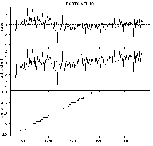
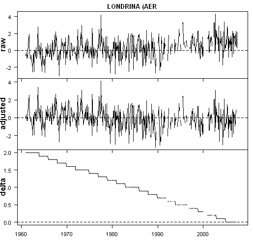
Porto Velho and Londrina are two somewhat similar sized Brazilian cities (populations 335,000 and 500,000 respectively) which have remarkably different Hansen adjustments. One is adjusted up by 2 deg C and one is adjusted down by 2 deg C. It’s pretty strange to see.
One of the advantages of having gone to the considerable effort of collating raw and adjusted Hansen versions is that some statistical comparisons can be carried out. In this case, I was intrigued by the following Hansen et al 2001 claim:
Indeed, in the global analysis we find that the homogeneity adjustment changes the urban record to a cooler trend in only 58% of the cases, while it yields a warmer trend in the other 42% of the urban stations. This implies that even though a few stations, such as Tokyo and Phoenix, have large urban warming, in the typical case, the urban effect is less than the combination of regional variability of temperature trends, measurement errors, and inhomogeneity of station records.
For all GHCN-“urban” sites (not claiming that GHCN-“urban” is coextensive with any rational definition of “urban”) that had adjusted versions, I calculated the adjustment by site and then the trend in the adjustment. I then looked at Brazil which we posted on before and picked two similar cities with strong opposite adjustment trends for spot checking.
Porto Velho
According to Wikipedia, “Porto Velho (-8.77 -63.92) is the capital of the Brazilian state of Rondônia, in the upper Amazon River basin. The population is about 334,661 people. …Porto Velho’s modern history begins with the discovery of cassiterite around the city, and of gold on the Madeira River, by the end of the fifties. Also, the government’s decision to allow large cattle farms in the territory began a trend of migration into the city. Almost one million people moved to Rondônia, and Porto Velho’s population increased to three hundred thousand. This intense migration caused much trouble for the city. For example, the suburban boroughs are nothing but shanty towns, among many other problems.”

Here is a plot of the GISS raw, GISS adjusted and net adjustment for Porto Velho. In this case, Hansen’s adjustment has the effect of lowering reported temperatures in the 1960s by up to 2 deg C.
Londrina
Again, according to Wikipedia, “Londrina (-23.33 -51.13) is a city located in the northern region of the state of the Paraná, Brazil, and is the 369 km away from the capital, Curitiba. Londrina exerts great influence on Paraná and south region. Londrina has approximately 500 thousand inhabitants, being the second largest city of Paraná and the fourth largest city of the South Region of Brazil.”

Once again, here is a plot of the GISS raw, GISS adjusted and net adjustment for Porto Velho. In this case, Hansen’s adjustment has the effect of increasing reported temperatures in the 1960s by up to 2 deg C.
Returning now to Hansen’s argument that urbanization did not “matter”:
Indeed, in the global analysis we find that the homogeneity adjustment changes the urban record to a cooler trend in only 58% of the cases, while it yields a warmer trend in the other 42% of the urban stations. This implies that even though a few stations, such as Tokyo and Phoenix, have large urban warming, in the typical case, the urban effect is less than the combination of regional variability of temperature trends, measurement errors, and inhomogeneity of station records.
In this case, Hansen does not appear to have made any concerted effort to ensure that the Brazilian “rural” stations are actually “rural stations; any more than he attempted to ensure that U.S. stations met even gross quality control specifications. Hansen’s methodological description says that their adjustments coerce trends at individual stations to the trends of “rural” stations within 1000 km. The Brazilian “rural” stations are not really rural stations and, in some cases, appear to be urbanizing just as fast as “urban” stations. So if the non-climatic contamination at the reference stations is changing at approximately the same rate as the non-reference stations (which is a very obvious possibility), then trivially one would find that the adjustment of non-reference stations would be more or less evenly distributed about the trend.
,


59 Comments
Steve – good post. One nit, looks like you have an extra zero typo in the first paragraph. I think Londrina should be 500,000, not 5 million. It’s correct further down the page.
population history here
http://www.populstat.info/Americas/brazilt.htm
Kudos to Jan Lahmeyer for collating.
Since Hansen uses 1980 population it might be intersting t look at which
locations on his list have the bigest varience frm 1980 figures
Are the charts the wrong way around? That is, is the Porto Velho triple-chart actually the Londrina triple-chart, and vice versa?
(Or am I out of my depth again?)
Do I misunderstand, or are you (Steven Mosher) saying that Hansen uses 1980 population data, and extrapolates corrections to the present time ? On what basis ? If the population growth is roughly the same, shouldn’t the corrections be roughly the same ? I am reminded of Joe D’Aleo’s (ICECAP) data for NYC (Central Park) showing no trend in the raw data, but a steadily increasing growth in the GISS corrected data. What ever happened in NYC ?
#5. I figure out the NYC thing. It was a total fiasco even by climate science standards. The NOAA “urban adjustment” in effect de-populated NYC between 1990 and 2006 to 1870 levels and then “corrected” the urban-adjusted number for the de-population.
I’ve been working through the Brazil thing some more – what a joke. There are 8 Brazil stations that are “GISS-rural”, have values that begin for 1960 and end after 1990 (so that there is a 1960-1990 “normal”). For all 8 stations, there are no adjustments. I presume that HAnsen is more or less coercing all of Brazil to these 8 stations or some variation. The 8 qualifying stations are:
“SAO GABRIEL D[a Coheira]”
“BENJAMIN CONS[tant]”
“BARRA DO CORD[a]”
“QUIXERAMOBIM”
“CRUZEIRO DO S[ul]”
Conceição d[o Araguaia]
CARAVELAS” ”
Santa Vitória d[o Palmar]
If you look at Bernie’s population growths, these are among the most explosive population growth areas. Cruzeiro do Sul has a population of over 85,000. These are Hansen’s “rural” stations ??? What a Gong Show.
Steve, I don’t have the bandwidth to download it, but I was wondering whether there is any evidence in the raw GISS data suggesting any significant rise in the contiguous US temperature ? Or is the purported rise due primarily to adjustments ?
Well, the only reason to apply those kinf of adjustments would be if one wanted to show a small gradual increase in the southern hemisphere temperatures.
Homogeneity adjustments should not come anywhere near 2.0C and Hansen is not using a 2.0C urban warming adjustment so this would be nothing but chart/data trend selection adjustments.
(X-axis starts at 1960?)
(Steve McIntyre says:
August 26th, 2007 at 4:42 pm)
“I figure out the NYC thing. It was a total fiasco even by climate science standards. The NOAA urban adjustment in effect de-populated NYC between 1990 and 2006 to 1870 levels and then corrected the urban-adjusted number for the de-population.”
Steve: Does NOAA agree that they did this?
Thanks,
Dan Blachly
Steve McIntyre says:
August 26th, 2007 at 4:42 pm
“If you look at Bernies population growths, these are among the most explosive population growth areas. Cruzeiro do Sul has a population of over 85,000. These are Hansens rural stations ??? What a Gong Show.”
Seeing you as the gold standard for the skeptics, it pains me to see you use insults. Understand your frustration, though.
Dan Blachly
I have to say that this whole issue of the adjustments has me perplexed. From what I can tell, the adjustment process serves no meaningful purpose. I believe we would do just as well to ignore the urban stations entirely and simply base our computations on a fewer number of “high quality” stations (if they indeed exist, which I’m beginning to wonder).
To explain my concern, consider a single station located in the center of a city surrounded by 4 rural stations. Our goal is to determine a trend of the aggregate data. The trend data is reflective of the low frequency components in the data where the frequencies of interest have periods of many months to many years. We really have little interest in the higher frequency data (periods of hours, day, or weeks). Each station will have some mean temperature and the actual temperature will have a variance about that mean. It seems to me, the reason we want to integrate the results from multiple stations is to reduce the variance of our measurements to eliminate spurious or localized trends. So far, I don’t think I’ve said anything controversial.
BUT, it seems that our adjustment process wants to replace the trend found at the urban location with the aggregate trend of the 4 surrounding rural stations. This is in essence, replacing its low frequency content with that of the other stations. Therefore, the urban station is no longer statistically independent. (Think of having 1 station and using it’s data twice, you don’t get half the variance). Including it in the composite measurement has no effect on the resulting variance. We would do just as well by ignoring the urban sensor and just using the 4 rural sensors. In other words, the urban station measurements no longer have any meaningful information content.
It seems as though the only reason to use these adjusted stations is it provides for a far more impressive station count. Can someone straighten me out here?
I agree. Surely this has been done (at least on a small scale).
Forgive me for being such a novice, but are there not atmospheric temperature references from which to compare to? I am beginning to get beaten down by all of the adjustments, urban heat islands, and poor HCN monitoring stations.
Hansen is looking more and more like a incompetent buffoon rather than a respected climate scientist.
A bit of a side note, but has anyone figured out why GISS uses that strange stairstep correction? The correction looks basically linear over time, why not apply a smooth correction instead of the step function?
The fact that the correction does appear somewhat linear over time is also difficult to explain. If my memory is correct, the Karl UHI correction was an exponetial function of population growth, not linear. A station move should have a single step correction. The only reason I can think of for a linear correction is that you want to force two points spaced in time to specific values and spread the correction evenly between them.
#11. It’s not relevant whether NOAA “agrees” or not – here’s the evidence http://www.climateaudit.org/?p=1798 .
#15. The KArl UHI correction is not used in the USHCN or GHCN “adjusted” data. It only uses the TOB and station history adjustments, with the latter one looking particularly pernicious.
Jeff at 7.28:
I suspect steps are used so that every reading in an interval will get the same adjustment. Otherwise a calculation would be needed for each event.
Using steps can also make it appear you know what you are doing. Just vary the steps slightly and people will think you really put some deep thought into each increment.
But your last sentence is probably right; a linear adjustment may be the best you can do in a given circumstance. Unless or until the method is explained we can’t know.
re #11
Steve is not directly insulting the individuals, he’s saying that if these individuals were performing on the GONG SHOW with their ‘science show’, they would be GONGED and rightly so! Ad hom’s are not Steve’s style, unlike Hansen and his ‘Jester’ quote amongst others.
LOL, another clusterf–k. I don’t see how anyone can have any faith in the “global average surface temperature,” anymore. It’s hillarious, in a weird way.
Re 17
Now I’m really puzzled. It the adjusted data only includes TOBS and station move/history changes, aren’t these events that happen at a discrete point in time? The correction should only be a couple of steps corresponding to the date of the change. The adjustment shouldn’t take place in 20 0.1 degree steps spread over decades. (BTW, the stairstep appears to be single decimal place rounding.)
The only reason I can think of for smearing the correction over time is to hide an obvious discontinuity the correction adds to the data. Since the step correction is intended to remove discontinuities introduced from instantaneous location/methodology changes, something seems very odd.
After my last comment, I went back and re-read the data description at the GISS website. It speaks of the three data sets:
1) Raw GHCN – I assume this means no adjustments whatsoever (except maybe TOBS?)
2) After combining sources at the same location – I take this to mean that mutliple sites are strung together over time to make one continuous data record over the last 100 years or so. I assume this is where station move adjustments would take place. I assume this correction is determined based on the overlapping data.
3) After Homogenity adjustment – this seems to be where urban sites are coerced toward rural trends
Can anyone confirm my interpretation? Do the plots above speaking of raw vs. adjusted compare #1 vs. #2 or #1 vs. #3? If its #1 vs. #3 the the phased-in correction makes more sense. However, if the “rural” site has a bias (i.e. it’s not rural or has microsite issues) the correction is questionable.
Any clarifications would be greatly appreciated.
Agree with #12 why not just use “real rural” from 1880 to 2007. Even though they may be few are far between, the stations seem to be well distributed worldwide. VG
1) For USHCN, they do not use raw GHCN, they use adjusted USHCN other than post 2000 when they use raw GHCN and fudge a year 2000 step (they should have just used USHCN adjusted but seem to be too stubborn)
2) Not necessarily. There are two things going on: many times their are different scribal sources so that there are overlapping versions often with identical values. I think that the major thing here is combining scribal sources, but it does get intermingled with stations as well as witness 20 year hiatuses.
3) GISS-“rural” is not necessarily rural. The Brazilian “rural” sites seem to be rapidly growing small towns and cities.
#23. Makes sense to me as well. Same in the U.S. Some of the USHCN stations are obviously decent and the composite of these sites is the next stage on this.
Re 24,
Thanks for clearing that up. With all the different dataset versions between GISS and NCDC, I don’t know how you keep them straight.
Here is the Porto Velho in terms of annual data:
a) Raw GHCN + USHCN corrections (showing individual stations)
http://data.giss.nasa.gov/cgi-bin/gistemp/gistemp_station.py?id=303828250005&data_set=0&num_neighbors=1
b) After Homogeneity adjustment
http://data.giss.nasa.gov/cgi-bin/gistemp/gistemp_station.py?id=303828250005&data_set=2&num_neighbors=1
c) Superimposing b) (in red) on a)
(Repeat of 27 – apologize for not putting in correct image display coding)
Here is the Porto Velho in terms of annual data:
a) Raw GHCN + USHCN corrections (showing individual stations)
http://data.giss.nasa.gov/cgi-bin/gistemp/gistemp_station.py?id=303828250005&data_set=0&num_neighbors=1
b) After Homogeneity adjustment
http://data.giss.nasa.gov/cgi-bin/gistemp/gistemp_station.py?id=303828250005&data_set=2&num_neighbors=1
c) Superimposing b) (in red) on a)
Hansen is looking more and more like a incompetent buffoon rather than a respected climate scientist.
There doesn’t seem to be much of a distinction at this point!!!!
SteveM
The graphs start at 1960. Am I misunderstanding?
Steve: My bad. Corrected.
#12 Schlew
I agree. In most instances in the US there are reasonable rural stations within a 100 KM of most defintively urban locations and these could form the basis of a more homogeneous dataset yet still ensure adequate coverage of regional climates. If Urban station data is included it should be weighted by the land area covered. Even in Brazil where only three genuinely rural sites out of 57 GHCN sites exist, there are over 300 weather stations not covered by GHCN. This suggests that while presumably there would be less historical coverage there would be a cleaner data set. At the moment the data set seems to have been constructed by the drunk who lost his car keys and was looking for them under the street light, because that is where he could see!! While this may be necessary in some scientific enterprises, i.e., we can only measure what we can measure, it hardly fits the bill here.
I still have a major concern about simply defining rural sites by population as opposed to visual inspection – hats of to Pielke and Watts – is that I think that local microsite changes caused by new buildings/heat sources in the immediate vicinity may be equivalent trend wise to UHI effects. If anyone has extracted the Canadian Arctic stations I suggest matching them up with dwelling counts, e.g., that can be obtained especially from Provincial and Canadian census data, e.g., Northwest Territory data is here. I was going to do it this weekend but had house guests.
Dwelling counts may make less sense for non-rural stations because the UHI trend effects may simply swamp micro-site trend effects. Although now that I write this, it is probably an open question.
Hans Erren:
Jan’s data is excellent and certainly shows the explosive growth of towns in Brazil. The notion that anyone is using 1980 figures to define rural stations is disturbing to say the least. Here is the source I used for the 2006 estimates for most municipalities. You click on the link on that page and get an Excel file.
#2 Hans:
Jan’s data is excellent and certainly shows the explosive growth of towns in Brazil. The notion that anyone is using 1980 figures to define rural stations is disturbing to say the least. Here is the source I used for the 2006 estimates for most municipalities. You click on the link on that page and get an Excel file.
Here is an alternative approach to the UHIE problem. For an analogy, consider measuring the temperature of a piece of heated metal where the heating is not uniform. You would take measurements over the surface at various points. Would you “adjust” hot spots relative to colder before averaging? No you would probably estimate the relative size of the area each temperature represented and weight them accordingly. Why are city temperatures adjusted? They are just as valid a measure as a rural temperature, the question is what area are they representative of? So my thought is instead of adjusting the temps based upon a guestimate of the affect of UHIE the temps are weighted based on the terrain they represent before averaging. The issue then becomes one of estimating the size of the area they represent. Any thoughts?
BarryW August 27th, 2007 at 7:22 am,
I don’t know if that would work well in places where the elevation changes rapidly. Sounds good for “flat” country.
BarryW, I’m pretty sure the assumption is that cities make up a tiny proportion of the total surface area of the planet (including oceans, etc), so UHI needs to be removed from the picture via some mechanism.
Barry, Simon and Pete
In a sense the 5X5 grid process Hansen and others use is meant to weight these urban stations, but it fails to do so if there are insufficient truly representative stations in a given grid cell. For example, if you wanted to measure the temperature of NYC, positioning the station in Central Park is not a good idea. If you wanted to measure the temperature of Southern NY State, it would be better, but not as good as West Point. So the issue is not urban or rural but the representativeness of where the stations are compared to the region that you want to measure. One should start with a map that plots out different climate areas, define grid sizes that across the globe minimize the amount of variability within these cells and then use the best stations in that cell that reflect the climate that the cell represents. NYC could in fact be a single cell given it geographic extent but then it would be avaraged with many more cells. It is akin to structured random sampling techniques that are pretty typical for household surveys run by the Bureau of Labor Statistics or well constructed opinion polls. The approach taken for the GISS is problematic because of the non-random distribution of weather stations and the lack of high quality stations.
Someone may know why they settled on 5 X 5 grids or other cell sizes – I suspect it is to do with the availability of data rather than the variabilty of climate.
#34 through 37,
I though the attempt to remove the UHIE was intended to distinguish the effects of global warming, purportedly from greenhouse gases, from the local urban effects, e.g., expanses of pavement. The areal adjustment approach would not seem to accomplish that.
Re #35, #36, #37 & #39
bernie I think your description is pretty much what I’m trying to say. The non uniform spacing of the sites is an issue. How do you characterize an area when you have no measurement that is representative of that area? Trying to define uniform climate areas seems like a good approach.
The problem I see with the way they are doing it is to try to determine an adjustment to account for the UHIE. Well my point is to stop trying to remove the local effect, at least with respect to the UHIE. The UHIE isn not really a bias, it’s still a valid measure of the temperature at that spot and the city still contributes heat to the system, but only on a local scale. The question is how big an area does that represent and how much should it be counted in the averaging? Consider the 5X5 grid. If the city where the measurement was taken comprises a .5X.5 area thats 10% of the total area and it’s contibution to the temperature of the 5X5 grid would be weighted accordingly. I would think it would be much more accurate to determine an area measurement than to estimate population based on lights, then adjust based on an estimate of the effect of population on heat generated (which would vary considerably based on the type of urban enviornment and the population density as opposed to size). The question of non uniform terrain is interesting. Does the present method account for terrain/climate variation? A measurement in the valley would not translate to the adjacent mountain in any case.
Barry:
My math says .5*.5 is 1% of 5*5 not 10%- otherwise I think we are in agreement. The issue remains that too many of the current
stations are “urban”. Correcting for this urban trend is only necessary because the urban trend is unrepresentative of the trends in the rest of the region as a whole, that is, the trend due to the immediate anthropogenic effects of asphalt, concrete, and
heat sources is confounded with trend dues to climate change. Ideally these sites should be disgarded in favor of regionally more representative sites, which in most grids will be non-urban sites.
#38
DeWitt
The UHI adjustment does in fact try to correct for this effect, the question is how can you do this. Currently they try to use rural stations to do this, but the question becomes why adjust rather than discard? The Brazil data provides part of the explanation – there are too many urban stations and we would be left measuring the temperature trend for Brazil using one station on an island in the South Atlantic. Since that is palpably foolish, they have no alternative than to try and adjust the data they do have. However, this is problematic because they need rural stations to do so. The “within a 1000 km” rule is a sign of how desperate they are to draw conclusions from seriously flawed datasets. The alternative is too claim that while there maybe an UHI effect there is no discernible UHI trend that is co-mingled with the climate trend. This allows for the preservation of the existing data set. The open questions are: (a) what is the UHI trend? (b) how many high quality rural stations exist? The battle for a clear view of the data and the adjustment methodologies is to answer these very simple questions. The building of a high quality climate network suggests, IMO, that these very smart guys actually know the answers to these questions, namely the current data and adjustments are seriously flawed. Unfortunately they are in a box where obstructionism appears to be an attractive alternative to coming clean with the limitations of their data-sets.
#7,
Steve Mc, if I read correctly, the urban stations are being co-erced to the rural station trends. My questions are:
1. Do the rural stations show any trend?
2. How many locations in the southern hemisphere would it take to determine if the same type of logic is being applied throughout.
3. Is it possible that the southern hemisphere not showing the same warming as the northern hemisphere is due to these types of adjustments (or lack thereof).
Adjusted data is a phrase incompatible with science.
You use the raw, “real”, data and scratch your heads over the results. Then, perhaps, you can explain them.
But, sorry, adjusting your “data” prior to the experiment in accordance with some belief concerning those data is wrong, wrong WRONG!
#41 Bernie, the satellite data is obviously the most global in scope and the most unaffected by UHI. Why is the GISS and IPCC not relying soley on these?
And BIM (Before It’s Mentioned), there is a 30 year record. We can correlate that 30 year record with the truly rural stations and extrapolate backwards – now there’s an awkwardism 🙂
If you have raw data and you can append meta-data reliably to each record it should be relatively easy to construct an alternative class of model to generate trends for comparison.
For instance, I would recommend starting with a pair naive model such as:
m1 = rawTemp ~ sitePopulation + microSiteClassCode + TOBSCode + …
and
m2 = rawTemp ~ year + sitePopulation + microSiteClassCode + TOBSCode + …
then diff the two models to get the trend (influence of year)
The idea here is to skip entirely the correlation and adjustment phase of the normal analysis and simply attempt to explain the raw temp as is using whatever meta-data you can reliably get your hands on. This could include current and historical micro site classification and any other kind of reliable globally consistent factor that can be attached to the data.
If the goal is to extract a temperature trend from a broad cross-section of data, I think it is somewhat misguided to even attempt to piece together a consistent long term data stream for each specific location prior to doing broad cross-section analysis. It is not necessary and it’s not obvious that it is adding to the accuracy of overall result.
On the other hand, if the goal is to accurately establish a temp history for a (large number) of specific locals then I agree that the current approach of correlating/adjusting individual streams makes sense.
(I would recommend doing the modeling with GBM in R for several reasons including that it will not then be necessary to actually have data for every factor or input in every record. Is is perfectly reasonable to plug in NA values where you don’t have a value and proceed. It will not bias the results one way or the other as long as you are fair with inclusion/exclusion of data)
Now, I may be completely missing the fact that this is routinely done but if so, feel free to ignore as needed.
#45, Gavin
Sorry but I am a little confused.
You said:
I beg to differ. You are assuming that one can accurately establish a temperature profile by adjusting data from different sites, and this is done, of course, to juxtapose apples to apples. It seems to me, the more we learn about apples, the less accurately we can say much about its core. There is too much error in the data such that any adjustment establishes reality. I for one do not trust that a temperature profile created by adjusts and splines is any better than the raw data.
Ian
Re # 12 schlew
Historically, we have only maximum and minimum temperatures in the main, when the physical factor of real interest is heat, or if possible, a representation of heat (watt per sq m) that can be approximated by working over many temperature measurements each day. We don’t have these until recently, so we are stuck with max and min. The average of these has not been shown in any of my reading to correlate well with watt per sq m. There are some days when it is briefly 40 deg C and other days where it is 40 deg C for several hours. The shape of the daily temperature curve is of interest but usually unavailable.
If you take a station that today is heavily urban, then take a group of stations surrounding that centre, it is possible to get some idea under ideal conditions of the UHI effect. The trouble is, you have to be able to work out when the UHI started, not only in the central station but also in those surrounding it. The reason is that one has to go back perhaps to the start of the 1900s to locate the start of UHI for cities that are large now. The reference stations need to have existed for a long time also, so their relativity over time can be calculated. There is thus a fair chance that the outlying stations have been grown over and have their own UHIs to correct. It is hard to find outlying stations that have had thermometers since 1900 but no nearby temperature growth. Why would one site a weather station in a wilderness for 100 years? Maybe some old mining sites will qualify, but these are an exception, not to be relied upon.
This is precisely the situation in my home town of Melbourne Australia, population about 3 million, where the city centre has records back to 1855, first settled about 1840. There are about 10 other stations from (say) 5 to 20 km out, with data from the 1950s typically, when some were paddocks and some were lightly settled.
Subtraction of the aggregate of these from the central station gives roughly a 1.5-2 degree C estimate of the central UHI magnitude. But, the raw data for Melb Central suggest that UHI could have started in the 1920s and the full extent might be another degree more.
There is very little good science that can be done with data like these. There are too many confounding variables of unknown extent. For example, one cannot simply take the population around a site as an estimator, when (unknown) population density might be a better measure. There is really no accuracy that I have seen in estimating how far apart two stations can be before they lose connectivity. I have proposed geostatistics to try to estimate the range, but have seen no results.
Further, nobody seems to know the significance of an average daily air temperature 1.5 m above the ground, in terms of extrapolating this to GLOBAL heat flow balance. It does not correlate well with sea temperatures, which can be measured at various depths and which are disturbed by currents. The corrections in both seem noisier than the real data movement and the situation is worsening under each new inspection.
The two solutions that appeal to me for existing surface land data are to scrap all readings where perturbations are suggested; and to correct nothing.
Those who retire in some years from now will not find it comforting to tell their grandchildren “I spent my careeer working out ways to correct temperature data that are not really capable of correction.” That’s work for losers.
Geoff:
I too think the satellite measures would make more sense, but I have much less of a feel for the issues surrounding those measures. Yet another subject to add to my already long list. The issue remains that many of the protagonists still push the station records. One either addresses them in their own terms or relinquish the field, even though their basic assumptions and logic may be seriously flawed.
Geoff Sherrington August 28th, 2007 at 4:30 am ,
At the risk of another deletion, I wish to point out that the best way to measure heat would be to measure temps at different levels in the ocean and the ground. With local velocity numbers for the ocean. Let the actual integrator tell you what the numbers are instead of estimating the heat capacity of the integrator.
Climate Science Needs To Go Underground
The heat capacity of the air is small and thus you can have large delta Ts from small changes in heat flow or air flow.
A more reliable measure of climate would be the actual temperature of the Earth. Not just the air (which is the least useful for climate).
M. Simon
Roger Pielke, Sr., of the soon to be defunct Climate Science web log, has proposed ocean heat content as the gold standard for years. Unfortunately, it isn’t very easy to measure and significant problems have been identified with past records. OTOH, a good measurement gives a relatively instantaneous measure of the overall radiative balance of the system.
Re: #37…”Someone may know why they settled on 5 X 5 grids or other cell sizes – I suspect it is to do with the availability of data rather than the variabilty of climate.”
Bernie,
Marsden squares have long been used by maritime/nautical organizations as a mapping system, and nautical meteorolgy has customarily used the Marsden square numerical designation systems (there are multiple variations) as a basis for reporting weather conditions. Marsden squares are quadrangles measuring 10 degrees of latitude by 10 degrees of longitude, and each Marsden square is allocated a numerical identifier. The WMO (World Meteorological Organization) further developed another system for numbering Marsden Squares and designated this 10 degree by 10 degree geocode system as World Meteorological Organization Squares. More recently, the C-Squares system of hierarchal geocodes was introduced by Tony Rees, CSIRO Marine Research, which further defines the Marsden Squares and WMO Squares in 5 degree, 1 degree, 0.5 degree, and smaller resolutions. Meterological satellite sensing systems have based much of their sensing data reports on these types of customary meterological geocodes to facilitate data management.
See:
Rees, Tony, CSIRO Marine Research, Hobart, Tasmania Australia. C-Squares, a New Spatial Indexing System and its Applicability to the Description of Oceanographic Datasets.
Click to access csq-article-Mar03-lowres.pdf
Re 40
Yeah, it’s 1%, moved a decimal point in my head. Been using a calculator too long. My contention is a compromise between thowing the urban sites away, and “adjusting” the temperature data. I think the urban data is still valid data, if treated properly, i.e., if it is representative of the area it represents and weighted properly. It’s the use of this data to represent areas that are not consistent with the area the temperature was taken in that I think is wrong. Also trying to adjust the data makes no sense since there is no accurate calibration for that adjustment, just rule of thumb. But on the other hand those sites are still representative of some of the earths surface and shouldn’t be ignored, just as a cold site shouldn’t.
D. Patterson (first name would make this less formal)
Excellent information. I am really intrigued that there may be satellite data out there that has the resolution needed to map urban centers (0.5 * 0.5) against their non-urban surrounding areas. One would have thought some bright (and fearless) PhD student would have nailed that one before now and we could have resolved this UHI issue with actual data.
RE: #14
“Hansen is looking more and more like a incompetent buffoon rather than a respected climate scientist.”
I don’t understand your comment. It sounds like you think those are mutally exclusive terms, when in practice the first term serves as a definition for the second term. 🙂
Re: #53
Note the application of C-Squares to “Oceanographic Datasets”…. Marsden Squares, WMO Squares, C-Squares and like meteorological geocodes are reported in the fields of some datasets and not in many others: often not in Surface and more often in some Marine, Upper Air, Satellite or Other datasets.
Try browsing the datasets:
Dataset Documentation
Click to access datasets.html
6380 – Worldwide Aircraft Reports, for one example, reports Marsden Squares.
Also note that Marsden Squares are sometimes reported in smaller divisions than 10 by 10 degrees by using Mesh Codes.
See for example:
Position Code Table
Marsden Square Chart (World)
Marsden Square Subdivisions
5 Degree Mesh Code
1 Degree Mesh Code
30 Minute Mesh Code
15 Minute Mesh Code
6 Minute Mesh Code
http://www.jodc.go.jp/data_format/position-code.html
While browsing and reading the dataset descriptions, note the presence and absence of data quality statements. See for example the comments about ASOS and issues with Platinum sensors having a range of inaccuracy and aspiration requirements.
Just a point to add. There is no reason why more rural stations could not be set up now as it is not as if the average temperature in a region is going to suddenly drop by 0.8 degrees. If there is a real warming trend and it has been increasing since 1987 then its hardly going to stop overnight. Measure at more rural sites for the next year with proper documented method and then see where we are.
If the ‘rural’ only data set matches the trend of previous observations then there is an increasing likelihood that there is real warming. If not then there is an increasing likelihood that there was no trend in the first place.
Why not call it the McIntyre criterion?
Perhaps they can have Anthony look at the new CDN sites before they go live? I am assuming that these new sites will be free from UHI effects.
Re #56
My understanding is that the USCRN (Climate Reference Network) is supposed to provide something of that nature.
RE 57.
The CRN has guidelines for site selection and guidelines for taking photos. I shared
these all a while back and I’m too damn lazy to do it again. So, google
NOAA CRN..
(Sorry bad mood flag is set positive.)
All the the CRN sites I have seen pictures of are pristine. From the sensor standpoint you
get 3 real time traces from 3 seperate sensors.
From a SPEC perspective I think the CRN addresses known issues. IMPLEMENTATION is the key.
Now, the papers supporting the CRN have been a little slow in coming out.
Anthony had a chance to talk with Baker ( at UCAR ) who is a key guy on CRN
THE BIG FIGHT will be this. How is the historcial network adjusted to the REFERENCE network.
And will changes get propegated to the past? for the US of course, 2% skim milk.