I’ve been trying for nearly a year to get a digital version of the Tornetrask reconstruction of Grudd (2008), also referred to in his thesis.
Last week, Hakan Grudd sent me a digital version of the MXD series – hooray! Previously I’ve previewed this new version using clips from the articles or thesis e.g here.
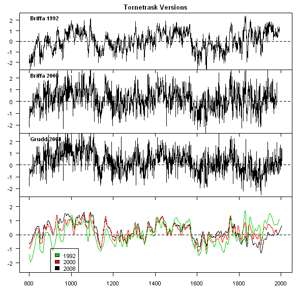
Because Tornetrask is used in every recon, I needed this new version to test the overall impact of the newer versions of key series. In the first figure below, I’ve plotted the three successive versions of Tornetrask – top, from Briffa et al 1992, the scene of what Per referred to as a “gobsmacking” adjustment, discussed here; middle from Briffa 2000, a version used in some later studies (though Juckes et al 2007 used the 1992 version on the pretext that “scientific” procedure mandated the use of older data) ; bottom – from Grudd 2008.
The three versions are overlaid in a smooth version in the 4th panel showing that the Grudd version has an elevated MWP relative to the modern period, that is not present in the Briffa versions.

Figure 1. Three versions of Tornetrask.
Next here is a figure showing the differences between the two earlier versions and the current Grudd 2008 version. Some people might even notice a little HS-ness in the difference between the two series.

Figure 2. Differences between Briffa versions and Grudd version.
In one of my earliest posts (before the Grudd version became available), I had noted that Briffa had “adjusted” his reconstruction and, as it happens, the amount of his adjustment is more or less equivalent to the difference between the Briffa 1992 version (used in many studies) and the present version. Thus some portion of the reconstructions using the Briffa 1992 version are an artifact.
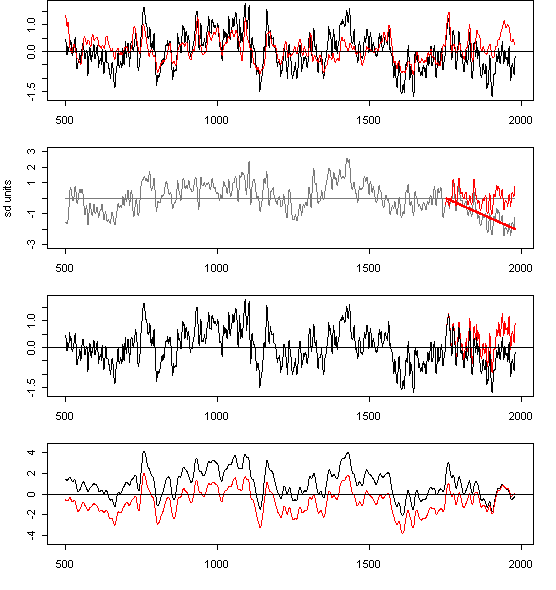
Here is the diagram that I presented in the earlier post.

Figure 3. Top panel: Tornetrask. RW (red) and MXD (black) chronologies. Second panel (compare to CD92 Figure 7): Black – residuals after regressing MXD against RW based on 500-1750; red line – “trend” of residuals after 1750; red – “adjusted” residuals. Third panel – “adjusted” MXD chronology after adding back “adjusted” residuals. Bottom panel – MXD chronologies with 1902-1980 zero (additional 25-year smooth). Black – unadjusted; red – “adjusted”. Note the change in 20th century relative to other periods.
In a recent post, I discussed Briffa et al 2008 (hot off the press), which included Tornetrask, mixed in some proportion with Finnish Lapland. As noted in my discussion of this post, no data was archived. I have just heard back from the journal and will profile this separately.
Here’s the figure from Briffa et al 2008. Squinting at it, it looks more like one of the earlier versions than the Grudd 2008 version. This could reflect the impact of blending Finnish Lapland data or it could be the use of an older Briffa version. Time will tell.

Original Caption: Briffa et al 2007 Figure 3. Regional curve standardized (RCS) chronologies (thin lines) and smoothed chronologies, the sum of the first three components of singular spectrum analysis of each RCS chronology (thick lines), for the regions: (a) Fennoscandia, … The grey shading represents the changing number of samples that go to make up the chronology through time.


19 Comments
Here’s an interesting aside:
Hooray comes from the Mongolian Hurree, used by Mongol armies and spread throughout the world during the Mongol Empire of the Thirteenth Century. In Mongolian Hurree is a sacred praise much like amen or hallelujah. (From Jack Weatherford. Genghis Khan and the Making of the Modern World. 2004)
THis is not turnkey as it uses info on my internal directories. But it shows the calculation and could be made turnkey at some point.
##TORNETRASK VERSIONS
url.Briffa< -"http://www.cru.uea.ac.uk/cru/people/briffa/qsr1999/qsrfig1.csv"
g<-read.csv(url.Briffa,fill=TRUE,skip=10,header=TRUE)#dim 1999×30
dimnames(g)[[2]]
range(g[,1])# 1 2000
id<-dimnames(g)[[2]]
id=800)
source(“d:/climate/scripts/treeconfig.functions.txt”)
#for smoothing function
torns=torn
for(i in 1:3) torns[,i]=filter.combine.pad(torn[,i],truncated.gauss.weights(21))[,2]
#PANEL PLOT SHOWING VERSIONS
nf=layout(array(1:4,dim=c(4,1)),heights=c(1.1,1,1,1.5))
ylim0=c(-2.5,2.5)
par(mar=c(0,3,2,1))
plot(c(time(torn))[temp],torn[temp,”1992″],type=”l”,xlab=””,ylab=””,axes=FALSE,ylim=ylim0)
axis(side=1,labels=FALSE);axis(side=2,las=1);box();abline(h=0,lty=2)
title (“Tornetrask Versions”)
text(790,2.2,”Briffa 1992″,font=2,pos=4)
par(mar=c(0,3,0,1))
plot(c(time(torn))[temp],torn[temp,”2000″],type=”l”,xlab=””,ylab=””,axes=FALSE,ylim=ylim0)
axis(side=1,labels=FALSE);axis(side=2,las=1);box();abline(h=0,lty=2)
text(790,2.2,”Briffa 2000″,font=2,pos=4)
par(mar=c(0,3,0,1))
plot(c(time(torn))[temp],torn[temp,”2008″],type=”l”,xlab=””,ylab=””,axes=FALSE,ylim=ylim0)
axis(side=1,labels=FALSE);axis(side=2,las=1);box();abline(h=0,lty=2)
text(790,2.2,”Grudd 2008″,font=2,pos=4)
par(mar=c(3,3,0,1))
plot(c(time(torn))[temp],torns[temp,”2008″],type=”l”,xlab=””,ylab=””,axes=FALSE,ylim=ylim0)
axis(side=1);axis(side=2,las=1);box();abline(h=0,lty=2)
lines( c(time(torn))[temp],torns[temp,”2000″],col=2)
lines( c(time(torn))[temp],torns[temp,”1992″],col=3)
legend(900,-1,fill=3:1,legend=c(“1992″,”2000″,”2008″),cex=1)
##PANEL PLOT SHOWING DIFFERENCES
nf=layout(array(1:2,dim=c(2,1)),heights=c(1.1,1.3))
ylim0=c(-2.5,2.5)
par(mar=c(0,3,2,1))
plot(c(time(torn))[temp],-torn[temp,”2008″]+torn[temp,”1992″],type=”l”,xlab=””,ylab=””,axes=FALSE,ylim=ylim0)
axis(side=1,labels=FALSE);axis(side=2,las=1);box();abline(h=0,lty=2)
title (“Tornetrask Differences”)
text(790,2.2,”Briffa 1992 less Grudd 2008″,font=2,pos=4)
par(mar=c(3,3,0,1))
plot(c(time(torn))[temp],-torn[temp,”2008″]+torn[temp,”2000″],type=”l”,xlab=””,ylab=””,axes=FALSE,ylim=ylim0)
axis(side=1);axis(side=2,las=1);box();abline(h=0,lty=2)
text(790,2.2,”Briffa 2000 less Grudd 2008″,font=2,pos=4)
Finnish Lapland tree-ring info is available from here:
Click to access MTP_231007.pdf
Click to access gt_trace2008h.pdf
Click to access gt_trace2008_cyclic.pdf
Click to access Cost725-2007.pdf
Click to access IsClimateChanging_MTP.pdf
Click to access holocene_trends.pdf
Click to access 7641pisyfi3G_MTP.pdf
Steve: The issue is not whether Finnish tree ring information is used. You’ve given a bunch of pdf’s; what is relevant is the rwl data set for the tree ring sites used in Briffa et al. Do you have a url for that data? One of the practices that academics really need to improve on is providing accurate data citations to the data, in addition to the print medium.
I’d forgotten how far back this particular proxy was discussed. Per was correct – if there’s any scientific justification for that procedure, then we should all give up now.
Actually this is a very interesting series. I am quite familiar with the Torne Träsk area and the scots pine is at the very edge of its distribution in this area and very sensitive to summer temperatures. The area is close to the Atlantic and has high rainfall, water stress is probably not much of a factor (which it probably is in the Finnish Lapland series, which are from a much drier area). Also there is a weather station nearby (guarenteed non-UHI) with an uninterrupted series from c. 1900 (which was the climax of the LIA in this area), so it is possible to correlate tree-ring and instrumental records over almost the whole temperature range of the tree-ring record.
In short, if there are any tree-ring records that are reasonable temperature proxies, this is one of them.
1) I am baffled by the Briffa adjustment explanation included in the previous related post. What exactly was it that justified alteration of only the most recent portion of the data? Was there some parallel table of historical measures of nitrogen availability?
2) Thanks to Sean for that very interesting bit about “Hooray.” I believe the Mongols were also among the first to use the word “Consensus” to mean “agree with me or you deserve to die” so it all kinda ties in with the climate thing.
This could be beginning of the end of NASA GISSTEMP?
http://www.telegraph.co.uk/opinion/main.jhtml?xml=/opinion/2008/07/27/do2708.xml
a pretty major story in the telegraph. Mentions (prominently) Anthony Watts and Steve
and CSIRO climate division as well?
http://blogs.news.com.au/heraldsun/andrewbolt/index.php/heraldsun/comments/csiro_heavy_says_dont_trust_csiros_scares/
what a coincidence! (re recent blogs here)
it would be so cool if you could add a monthly updated graph with the latest month’s data included. it would probably highly boost your hits too (if you even care about that!) because it would be the only place i know about that kept such a thing. i would love to be able to show the latest global warming graph with july’s temperatures included for instance.
just a suggestion!
mark
ps i made the same suggestion to anthony watts…..just now.
But this can’t be right. MWP > CWP. CWP is not uuuuuuuunprecedented.
tty writes
“In short, if there are any tree-ring records that are reasonable temperature proxies, this is one of them.”
hmm, that may be so from a theoretical dendro perspective. But science is empirical.
So why did Briffa have to resort to a post-hoc data manipulation to “show” that these trees are a temperature proxy ?
per
per:
Probably because the revised and un-fudged version shows both the MWP and the warm period in the 1730’s-1740’s significantly warmer than the present.
Yes, the theory is great, and indeed beautiful. However, the NAS/NRC panel agreed that the error associated with these reconstructions was unquantifiable; which is pretty severe. Our host has written more eloquently than I could on some of the tree-ring studies.
As to Briffa’s motivations, it is a pretty shocking thought to imagine that a scientist would manipulate data to get rid of a result that they didn’t like.
bring in GLP for environmental science…
per
Glad to know that you have succeeded in obtaining the Tornetrask data in a digital form, and I have enjoyed looking at your analyses.
Is there a chance of you providing a link to it? I realise that it may have been sent /privately/ to you. If so, please disregard my question!
Robin
per,
Actually a scientist wouldn’t manipulate data to get rid of a result that they didn’t like. This unfortunately leads to only one conclusion.
Re: (#3) Akseli:
July 25th, 2008 at 9:51 pm
I’ve yet to see this tree-ring-data from J.Meriläinen and M.Timonen on CA: SAIMA. They’ve archived data from 42 sites, but I’m not sure if data used in Briffa et al. is included.
The Tornetrask series seems to show a significant temperature maximum 1400-1500. This is the time of the deep Spoerer Minimum in solar activity. Stuiver and Quay (1980) point out that the cosmic ray flux during the Spoerer minimum was even higher than during the Maunder minimum. This puts to rest the argument that the low-temperature LIA was caused by low solar activity and high cosmic ray flux, if we adopt accept Tornetrask as being representative of global conditions…
Re: Leif Svalgaard (#17),
Leif: Don’t tell me you are now reading the tree rings!
(#17) Leif
According to wikipedia the Spoerer Minimum was between 1420 to 1570 or 1450 to 1550. This appears to corresponds with a rather rapid drop in temperature and a stabilization at a new level.