t-Statistics and the “Hockey Stick Index”

In MM05,  we quantified the “hockeystick-ness” of a series as the difference between the 1902-1980 mean (the “short centering” period of Mannian principal components) and the overall mean (1400-1980), divided by the standard deviation – a measure that we termed its “Hockey Stick Index (HSI)”.  The histograms of its distribution for 10,000 simulated networks (shown in MM05 Figure 2) were the primary diagnostic in MM05 for the bias in Mannian principal components.  In our opinion, these histograms established the defectiveness of Mannian principal components beyond any cavil and our attention therefore turned to its impact, where we observed that Mannian principal components misled Mann into thinking that the Graybill stripbark chronologies were the “dominant pattern of variance”, when they were actually a quirky and controversial set of proxies.

Nick Stokes recently challenged this measure as merely an “MM05 creation” as follows:

The HS index isn’t a natural law. It’s a M&M creation, and if I did re-orient, it would then fall to me to explain the index and what I was doing.

While we would be more than happy to be credited for the simple concept of dividing the difference of means by a standard deviation, such techniques have been used in the calculation of t-statistics for many years, as, for example, in the calculation of the t-statistic for the difference of means.   As soon as I wrote down this rebuttal, I realized that there was a blindingly obvious re-statement of what we were measuring through the MM05 “Hockey Stick Index” as the t-statistic for the difference in mean between the blade and the shaft.  It turned out that there was a monotonic relationship between the Hockey Stick Index and the t-statistic and that MM05 histogram results could be re-stated in terms of the t-statistic for the difference in means.

In particular, we could show that Mannian principal components produced series which had a “statistically significant” difference between the blade (1902-1980) and the shaft (1400-1901) “nearly always” (97% in 10% tails and 85% in 5% tails).  Perhaps I ought to have thought of this interpretation earlier, but, in my defence, many experienced and competent people have examined this material without thinking of the point either. So the time spent on ClimateBallers has not been totally wasted.


t-Statistic for the Difference of Means 

The t-statistic for the difference in means between the blade (1902-1980) and the shaft (1400-1901) is also calculated as the difference in means divided by a standard error: a common formula computes the standard error as the weighted average of the standard deviations of the two subperiods, weighted by the length of each subperiod.  An expression tailored for the specific case is shown below:

se= sqrt( (78* sd( window(x,start=1902) )^2 + 501* sd( window(x,end=1901))^2 )/(581-2) )

For the purposes of today’s analysis, I haven’t allowed for autocorrelation in the calculation of the t-statistic (allowing for autocorrelation will reduce the effective degrees of freedom and accentuate results, rather than mitigate them.)

Figure 1 below shows t-statistic histograms corresponding to the MM05 Figure 2 HSI histograms, but in  a somewhat modified graphical style:  I’ve overlaid the two histograms, showing centered PC1s in light grey and Mannian PC1s in medium grey. (Note that I’ve provided a larger version for easier reading – interested readers can click on the figure to embiggen.)   The histograms are from a 1000-member subset of the MM05 networks and a little more ragged.   I’ve also plotted a curve showing the t-distribution for df=180, which was calculated from one of the realizations. This curve is very insensitive to changes in degrees of freedom in this range and I therefore haven’t experimented further.

The separation of the distributions for Mannian and centered PC1s is equivalent to the separation shown in MM05 Figure 1, but re-statement using t-statistics permits more precise conclusions.

tstat_histogram

Figure 1. Histograms of t-statistic for difference of 1902-1980 mean and 1400-1901 means showing centered PC1s (light grey) and Mannian PC1s (medium grey). The curve is a t-distribution (df=180).   The red lines at +- 1.65 and +-1.96 correspond to 90% and 95% two-sided t-tests. 

The distribution of the simulated t-statistic for centered PC1s is similar to a high-df t-distribution, though it appears to be somewhat  overweighted to values near zero and underweighted on the tails: there are approximately half the values in the 5% and 10% tails that one would expect from the t-distribution.  At present, I haven’t thought through potential implications.

The distribution of the simulated t-statistic for Mannian PC1s bears no relationship to the expected t-distribution.  Values are concentrated in the tails: 85% of t-statistics for Mannian PC1s are in the 5% tails ( nearly 97% in the 10% tails.)  This is what was shown in MM05 and it’s hard to understand why ClimateBallers contest this.

What This Means

The result is that Mannian PC1s “nearly always” (97% in 10% tails and 85% in 5% tails) produce series which have a “statistically significant” difference between the blade (1902-1980) and the shaft (1400-1901).   If you are trying to do a meaningful analysis of whether there actually is a statistically meaningful difference between the 20th century and prior periods, it is impossible to contemplate a worse method and you have to go about it a different way.   Fabrications by ClimateBallers, such as false claims that MM05 Figure 2 histograms were calculated from only 100 cherrypicked series, do not change this fact.

The comparison of the Mannian PC histogram to a conventional t-distribution curve also reinforces the degree to which the Mannian PCs are in the extreme tails of the t-dstribution.   As noted above (and see Appendix), the t-stat is monotonically related to the HSI:  rather than discussing the median HSI of 1.62, we can observe that the median t-stat for Mannian PC1s is 2.44, a value which is at the 99.2 percentile of the t-distribution.  Even median Mannian PC1s are far into the right tail.  The top-percentile Mannian PC1s illustrated in Wegman’s Figure 4.4 correspond to a t-statistic of approximately 3.49, which is at the 99.97 percentile of the t-distribution.  While there is some difference in visual HS-ness, contrary to Stokes, both median and top-percentile Mannian PC1s have very strong HS appearance.

Stokes is presently attempting to argue that representation of a network through a biased Mannian PC1 is mitigated in the representation of the network, by accommodation in lower order PCs. However, Stokes has a poor grasp on the method as a whole and almost zero grasp of the properties of the proxies.  When the biased PC method is combined with regression against 20th century trends, the spurious Mannian PC1s will be highly weighted.  In our 2005 simulations of RE statistics (MM05-GRL, amended in MM05 (Reply to Huybers – the Reply containing new material), we showed that Mannian PC1s combined with networks of white noise yielded RE distributions that were completely different than those used in MBH98 and WA benchmarking.  (WA acknowledged the problem, but shut their eyes.)

Nor, as I’ve repeatedly stated, did we argue that the MBH hockeystick arose from red noise: we observed that the powerful HS-data mining algorithm (Mannian principal components) placed the Graybill stripbark chronologies into the PC1 and misled Mann into thinking that they were the “dominant pattern of variance”.  If they are not the “dominant pattern of variance” and merely a problematic lower order PC, then the premise of MBH98 no longer holds.


Appendix

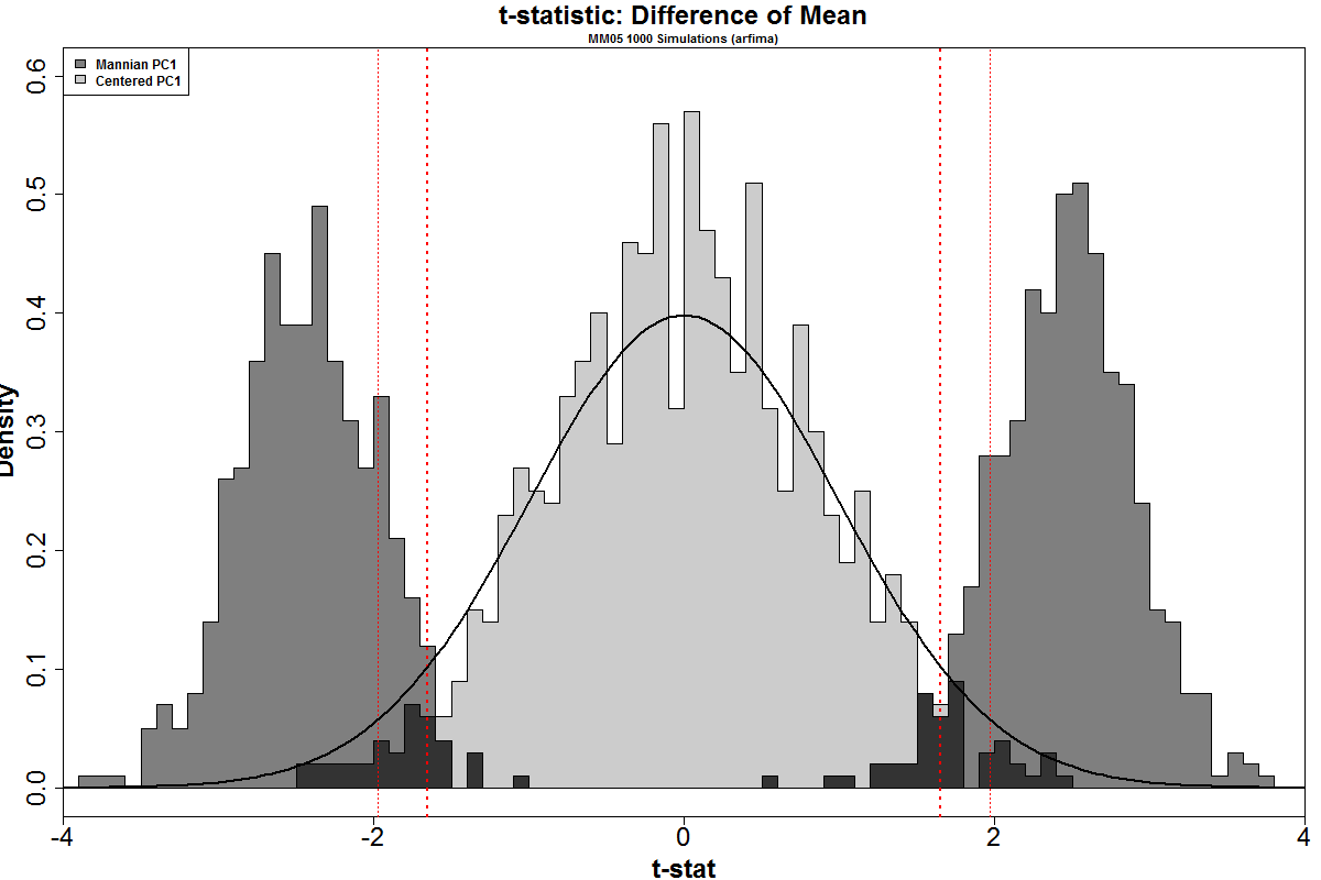
Figure 2 below compares the t-statistic for the difference between the means of the blade (1902-1980) and the shaft (1400-1901) against the HSI as defined in MM05-GRL: it shows a monotonic, non-linear relationship.  It is immediately seen that there is a monotonic relationship between HSI and t-statistic, with the value of the t-statistic being closely approximated by a simple quadratic expression in HSI.  The diagonal lines show where both values are equal.  The HSI and t-statistic are approximately equal for HSI with absolute values less than ~0.7.  Values in this range are very common for centered PC1s but non-existent for Mannian PC1s, a point made in MM05.

The vertical red lines show 1 and 1.5 values of HSI (both signs); the horizontal dotted lines show 1.65 and 1.96 t-values,  both common benchmarks in statistical testing (95% percentile one-sided and 95% two-sided, 97.5% one-sided respectively.)  HSI values exceeding 1.5 have t-values well in excess of 2.


tstat_vs_HSI

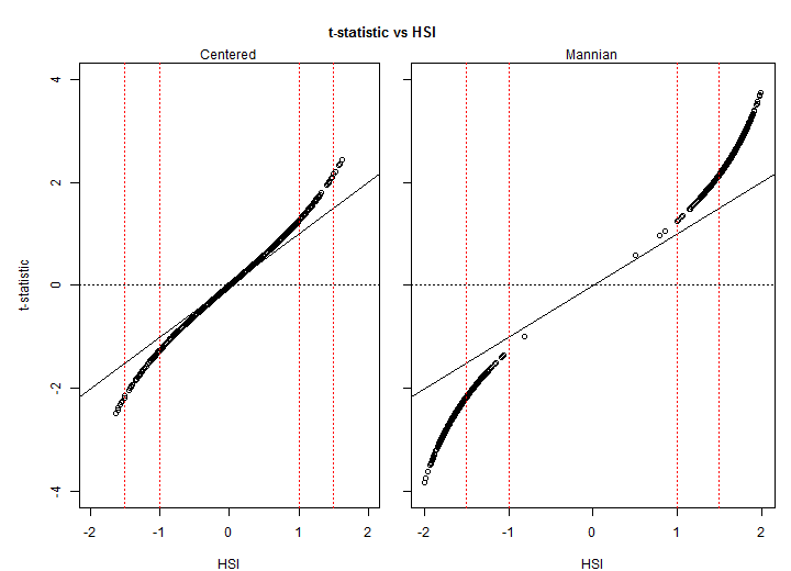
Figure 2.  Plot of t-statistic for the difference in means of the blade (1902-1980) and the shaft (1400-1901) against the HSI as defined in MM05-GRL for centered PC1s (left) and Mannian PC1s (right). It shows a monotonic, non-linear relationship.  The two curves have exactly the same trajectories when overplotted, though values for the centered PCs are typically (absolute value) less than about 0.7 HSI, whereas values for Mannian PCs are bounded away from zero.


193 Comments

  1. Posted Sep 28, 2014 at 3:47 PM | Permalink

    Wow. That’s impressive, Steve. I don’t know of a way to state your point more clearly and cleanly than what your plots show.

  2. TAG
    Posted Sep 28, 2014 at 4:29 PM | Permalink

    For very good reasons, I hesitate to comment on any technical posts here. Howver, even I see how conclusive this argument is and if someone like me can see it then that is very bad news for advocates of Mann’s methods

  3. Posted Sep 28, 2014 at 5:15 PM | Permalink

    I like this formulation of the problem. I think using t-statistics instead of your HSI makes things more accessible and intuitive.

    Plus you used the word “embiggen.” I love that word.

    • bill_c
      Posted Sep 29, 2014 at 11:53 AM | Permalink

      Brandon,

      How’s your Spanish?

      http://es.wikiquote.org/wiki/Jebediah_Springfield

      • Posted Sep 29, 2014 at 12:17 PM | Permalink

        I’m okay with the grammar and syntax in Spanish, but my vocabulary is terrible. I happen to know the reference though. That article is about a historical character in The Simpsons, quoted as having said, “A noble spirit embiggens the smallest man.” The word was made up for an episode of the show (as was “cromulent”), though it turns out it had been used at least once over a hundred years before.

        That’s a large part of why I love the word. What other word was jokingly created for a television show then accepted into the lexicon only to have people discover it may have been there all along?

        • bill_c
          Posted Sep 29, 2014 at 12:44 PM | Permalink

          And translated into Spanish as a new word (“agrandece”) which may also be an unofficial real word in some parts.

          It just sounds better when the Mexican guy with the deep voice says it.

        • Gary
          Posted Sep 29, 2014 at 5:01 PM | Permalink

          Anvilicious?

  4. Spence_UK
    Posted Sep 28, 2014 at 5:17 PM | Permalink

    I really just don’t understand why people try to defend Mann’s work and methods. And it isn’t just racehorse Nick – I’ve come across people trying to resurrect Mann’s work across the interwebs.

    How anyone can see a method that takes in data with a population mean of zero, and ends up with a bimodal distribution in the histogram where the sample mean appears allergic to zero, and think that this is an acceptable method, is just beyond me.

    Well known individuals who have some respect within this debate, e.g. Ian Jolliffe and Michael Liebreich, have expressed frustration at those who try to defend Mann’s work. Defending such obviously flawed methods surely does more harm than good to those who want to claim the support of objective scientific research.

    Steve: it really defies credulity. It really is hard to imagine a worse method for what they were trying to do. If someone used a similarly flawed method in (say) a chemistry paper, it’s hard to imagine other specialists rallying behind the offender or the journal not requiring major corrections, if not retraction, by the author.

    • MikeN
      Posted Sep 28, 2014 at 5:44 PM | Permalink

      I suspect it is two things interacting, as to why Mann is being defended.

      1) ClimateBall, the point is to win and not concede anything.
      2) Models are too complicated for most people to audit. I could point out upside down usage in Kaufman with Excel and Acrobat.

  5. stevefitzpatrick
    Posted Sep 28, 2014 at 5:34 PM | Permalink

    Steve:
    “Nor, as I’ve repeatedly stated, did we argue that the MBH hockeystick arose from red noise”

    But if the Mannian method is fed red (pink) noise synthetic series, statistically similar to real proxies, would they also generate Mann-like hockey sticks, as Jeff Id has said?

    I can see that the methods are problematic, but I just can’t judge how much the presence of red (pink) noise in the proxy series potentially compromises the results.

    Put as clearly as I can: is the entire approach doomed to generate hockey sticks, no matter the input data?

    • Posted Sep 28, 2014 at 6:14 PM | Permalink

      No. MBH’s methodology cannot create hockey sticks out of nothing. There has to be a hockey stick somewhere in its data. What MBH does is mine for any hockey stick, anywhere in its data, and turn that into a hockey stick reconstruction.

      The NOAMER network has 70 series which go back to 1400 AD. About 15 of them contribute to the hockey stick shape in MBH’s NOAMER PC1. The other 55 are irrelevant.

      NOAMER PC1 is then combined with 21 other proxies, 20 of which do not have a hockey stick shape. One (known as Gaspe) has a hockey stick shape, though it is smaller than NOAMER PC1’s. Because MBH regresses proxies against the modern temperature record, these two proxies with hockey stick shapes cause the final result to be a hockey stick. The other 20 proxies are irrelevant.

      Put simply, the PCA process cherry-picks any hockey stick shapes in its data to create proxies with hockey stick shapes. A later step applied to all proxies cherry-picks hockey stick shapes within those proxies. If none of the data has a hockey stick shape, neither of these steps can cherry-pick a hockey stick signal. But if any of the data has a hockey stick shape, these steps will find it and create a reconstruction out of it.

      For a visual demonstration, look at this post. It shows all 22 proxies in the MBH network which extend back to 1400 AD. Only two of the 22 have a hockey stick shape, meaning MBH’s final results back to 1400 depend entirely upon less than 5% of their data.

      • k scott denison
        Posted Sep 28, 2014 at 6:22 PM | Permalink

        Thanks Brandon for the explanation and link. Remarkable is the kindest thing I can say.

        • Posted Sep 28, 2014 at 7:30 PM | Permalink

          No prob. I think the fact MBH regresses proxies against the instrumental temperature record deserves more attention than it gets. The PCA issue has drawn most of the focus in the debates I’ve seen, but I think it is a more minor problem.

          MBH’s faulty implementation of PCA trys to give you proxies with a hockey stick shape. Regressing proxies against the modern temperature record ensures if you have any proxy with a hockey stick shape, you’ll get a hockey stick reconstruction. They’re both forms of cherry-picking. They just mainfest differently.

          But a point that often gets missed is PCA is just used to create biased proxies. You can create a biased proxy set just by cherry-picking what data you use. Find a series with a hockey stick shape (e.g. Gaspe), decide to use it as a proxy, and MBH’s methodology will produce a hockey stick reconstruction. You don’t need PCA to do that. In other words:

          1) PCA produces hockey-stick shaped biased proxies.
          2) Rescaling proxies by regressing them against the modern temperature record creates a reconstruction biased toward having a hockey stick shape.

          You don’t need Step 1 for Step 2 to work. Step 1 just helps ensure you have a properly biased proxy for Step 2. There are other ways to get similarly biased proxies.

      • stevefitzpatrick
        Posted Sep 28, 2014 at 6:28 PM | Permalink

        Brandon,
        But red(pink) noise will always yield odd shaped series due to persistence, and some of these will mimic the target temps. Are you saying that Jeff Id is mistaken?

        • Posted Sep 28, 2014 at 7:23 PM | Permalink

          Not at all. I should have been clear my comment was answering your last question (which says “no matter the input data”), not your first question (which deals with red noise series). The point I was making is the MBH methodology cannot create a hockey stick out of nothing. It cherry-picks data with a hockey stick shape, but that requires there be data with a hockey stick shape.

          Now then, given enough red noise samples, you will find hockey stick shapes. The degree of persistence determines what proportion of the series will have such shapes. It could be 1 in 10 or 1 in 10,000 depending upon the amount (and type) of persistence you build into your noise. Its important to realize you won’t get a hockey stick in every red noise series.

          But it’s also important to remember the NOAMER network had 70 series in it (for 1400, there were more series for more recent periods). If your red noise series have a 1 in 10 chance of having a hockey stick shape, 70 draws is enough to have a very high probability of getting at least one hockey stick shape. If you have one, MBH’s methodology will cherry-pick it as the “dominant signal” for the 70 series.

          In other words, it’s not as simple as saying “red noise fed into MBH’s methodology will produce hockey sticks.” Red noise certainly can do that, but there are details and nuances that point misses. The most important point is at least some of your red noise series must have a hockey stick shape. If they do, MBH will cherry-pick them. If they somehow don’t, MBH will have nothing to cherry-pick.

        • j ferguson
          Posted Sep 29, 2014 at 5:57 AM | Permalink

          Brandon, thanks for a very clear explanation of what has, for me, been a bit murky.

          MBH finds hockey sticks – it is a hockey stick signal detector. If there is no hockey stick in the data it won’t invent one. But what about other shapes?

          Assuming that a hockey stick with an upright blade at the beginning could exist in the tree-data, will MBH miss it? With the blade turned down beginning or end? I suspect this isn’t possible in red or pink noise, or if possible extremely unlikely. Or is it? If unlikely wouldn’t that make red noise a bit weak as a comparison. Or maybe our red noise generating algorithms? You certainly could have a temperature series with blade up or down and at either beginning or end even if we ‘know’ we didn’t.

          I also assume that white noise is extremely unlikely to contain hockey sticks and that for some reason, red noise because of its expression of history is more analogous to tree rings and so is used for these comparisons. I’m sure this is obvious to the rest of you, but not to me.

          I apologize for burdening you with these questions which likely have been well-hashed already, but so far the topic has lacked the junior-high school level treatment which I could comprehend.

          Steve: You ask: “Assuming that a hockey stick with an upright blade at the beginning could exist in the tree-data, will MBH miss it? With the blade turned down beginning or end?” If one adds an artificial series to the NOAMER network with elevated 1400-1450 and includes it in the Mannian PC calculation in the actual network with stripbark bristlecones, the series will be flipped over in the PC1. I noted this property in MM05-EE, calling it “perverse”. I recall corresponding with Ritson about this. Ritson didn’t understand it and thought that that we were deceiving him on the point and grew very belligerent.

        • Posted Sep 29, 2014 at 8:52 AM | Permalink

          Steve:

          I noted this property in MM05-EE, calling it “perverse”. I recall corresponding with Ritson about this. Ritson didn’t understand it and thought that that we were deceiving him on the point and grew very belligerent.

          The anger had carried over to ‘Chris’ who I sat next to last Tuesday. Righteous anger at the deceptions of McIntyre and Wegman, no answer on why Mann didn’t mention these names and focused on Sarah Palin.

          Steve: The antagonism towards Wegman among Mann’s ClimateBallers is visceral. For example, in Mann’s Hockey Stick Wars, Wegman is mentioned more often than I am.

        • Posted Sep 29, 2014 at 10:15 AM | Permalink

          j ferguson, no prob. Red noise series can have a blade at the beginning about as easily as they can at the end (there’s a difference due to the wind up period). A blade at the beginning of the series will tend to have little effect on the results as the noise from other series will (partially) drown it out. A blade at the beginning will have a huge effect. And if the blade is turned down, it’ll just get flipped over.

          White noise has no persistence so we don’t expect to see curves like in a hockey stick. A purely random sample will rarely look like a hockey stick. The reason red noise produces hockey sticks is its persistence. Persistence basically means one data point will help determine the next data point. In nature, we expect many physical processes to create persistence. Tree growth of this year is not unrelated to tree growth of next year.

          There’s a question of how much persistence one should have in these series (and the exact nature of that persistence), but the effects described in the post will hold true for any amount (or type) of persistence. That question just determines how strongly they’ll show up. A small amount of persistence would mean a small tendency for your red noise series to produce hockey stick shapes, affecting how often you can successfully cherry-pick hockey sticks.

          But no matter the details of the red noise series one uses to test MBH’s methodology, the conclusion will always be the methodology is biased toward cherry-picking hockey stick shapes.

        • Follow the Money
          Posted Sep 29, 2014 at 5:23 PM | Permalink

          Brandon writes,

          It cherry-picks data with a hockey stick shape, but that requires there be data with a hockey stick shape.

          What 1000 year data set looks like a hockey stick? One could weight proxies which look like it to emulate it, or use the very data from that set to effectively replicate its HS shape and name it ‘temperature.” It could be just an amazing coincidence.. but I kinda think not.

      • Nick Stokes
        Posted Sep 28, 2014 at 7:13 PM | Permalink

        “What MBH does is mine for any hockey stick, anywhere in its data, and turn that into a hockey stick reconstruction.”
        No, it doesn’t. It aligns PC1 with a hockey stick pattern. That has virtually no effect on the reconstruction.

        You can see this in the MM05EE Fig 1, which does the recon with and without decentering. There is virtually no additional HS effect. There is a little difference at the other end, mainly due to the deletion of Gaspe cedars from 1400-1450.

        • Jean S
          Posted Sep 29, 2014 at 7:41 AM | Permalink

          You are just amazing. The whole dynamic range of the smoothed curve is about 0.5 degrees. Now there is about 0.3 degrees difference in the early 15th century, and you claim that there is “virtually no effect”! And no Nick, Gaspe cedars were not “deleted” they should have never been there. I think that has been gone through step by step with you at least a couple of times. Yet, you come up with the same old lie once again. Shame on you.

        • Steve McIntyre
          Posted Sep 29, 2014 at 8:59 AM | Permalink

          Below is Mann’s own original calculation of the effect of bristlecones and Gaspe on the MBH reconstruction. One of the contemporary shocks in discovering the CENSORED file was the discovery that Mann clearly knew the effect of stripbark bristlecones on his results, but instead of discussing this plainly in his response to MM03, submerged this in a discussion of North American dendro as a group. In addition, Mann had made large and false claims about the supposed robustness of his results to presence/absence of tree rings – an issue that Brandon is persistent in pointing to whenever discussion turns to fraud. And yet Mann baldfacedly accused us of a flawed calculation because our 2003 principal components had not known about Mann’s idiosyncratic “stepwise principal components” and inadvertently done a sensitivity test on exclusion of stripbark chronologies on early MBH steps.
          mann_2003_ee-problem_figure1

          This is a little more than the effect of centered PCs plus Gaspe, since the stripbark bristlecones still have an impact (though reduced) in centered PCs.

        • Jean S
          Posted Sep 29, 2014 at 9:12 AM | Permalink

          Steve, where is that figure from? And of course, all sharp-eyed ClimateBallers noticed that Mann did not use the trick in the smooth (40 years smoothing as in MBH99).

          Steve: Mann’s contemporary reply to MM03:
          http://www.climateaudit.info/pdf/mann/EandEPaperProblem.pdf

        • Steve McIntyre
          Posted Sep 29, 2014 at 9:43 AM | Permalink

          Jean S,
          here’s another version that you probably haven’t seen and which deserves more discussion. In this version, Mann shows the separate effects of the stripbark PC1 and the Gaspe series, both of which are problematic. The scale of the early 15th century is reduced from the version that he placed online at the time.

          2003 mann submission to climchg figure 2

          This is from an article by Mann et al submitted to Stephen Schneider at Climatic Change in late 2003 and extensively discussed in CG1 emails in early 2004. I was asked to review it and, as a reviewer, asked Mann to provide the data that he had refused to provide me previously. This caused consternation among the Climatic Change editorial board, which included Phil Jones and Peter Gleick. Indeed, Gleick’s first appearance in Climategate is as a supporter of data obstruction, even to reviewers.

          Mann eventually refused to provide the data and appears to have abandoned the submission. By that time, he had done a check-kited citation in Jones and Mann 2004, which cited the submission as authority for trashing us. I’ll send you a copy.

        • Nick Stokes
          Posted Sep 29, 2014 at 7:48 AM | Permalink

          There’s some difference pre-1700. But since then, barely 0.1°C anywhere. Where are all those 20th Cen hockeysticks that were mined?

        • Nick Stokes
          Posted Sep 29, 2014 at 8:26 AM | Permalink

          Here is a version of Fig 1 from MM05EE with the centered and decentered superimposed. Since 1800, the differences are tiny. Mined hockey sticks?

          Steve: Nick, Mannian inverse regression is another chapter in the laboratory of horrors that is MBH. It hugely overfits the networks in the calibration period, resulting in highly inflated calibration r2 and calibration RE statistics – a point that I’ve made in the past.

        • Sven
          Posted Sep 29, 2014 at 8:28 AM | Permalink

          Correct me if I’m wrong, but my understanding has been that the whole “point” of the hockey stick was not the blade but the handle. So pre-1700 IS relevant!

        • Nick Stokes
          Posted Sep 29, 2014 at 8:51 AM | Permalink

          Yes, but the effect of the decentering is to cause PC1 to tend to have a jump at the start of the calibration period. We’ve been shown many pictures of that. But it’s just aligning one PC with that effect. The others are pushed orthogonal. So when you compare the recons, that jump is very hard to see.

        • Posted Sep 29, 2014 at 10:21 AM | Permalink

          Nick Stokes, you boldly claim:

          “What MBH does is mine for any hockey stick, anywhere in its data, and turn that into a hockey stick reconstruction.”
          No, it doesn’t. It aligns PC1 with a hockey stick pattern. That has virtually no effect on the reconstruction.

          While flat-out ignoring the fact I discussed more than MBH’s faulty implementation of PCA. I discussed how MBH regressing proxies against the modern temperature period gives enormous weight to hockey stick shaped proxies while treating the rest as noise.

          Most people can understand the concept there are multiple steps in MBH’s methodology. Most people can understand a person who spends quite a bit of time clearly discussing two different steps feels both steps are important. Most people can understand when I specifically say the PCA step isn’t necessary for MBH to cherry-pick a hockey stick shape for its reconstruction, I mean there are problem beyond the PCA step.

          I suspect that’s because the point is simple. The only way I can see not to understand it is to try very hard not to.

        • Posted Sep 29, 2014 at 12:10 PM | Permalink

          Is anyone else amused by Nick Stokes’s attempted defense:
          [Jean S: It would be hilarious if it were not so sad. This has been going on for years with no end in sight.]

          Here is a version of Fig 1 from MM05EE with the centered and decentered superimposed. Since 1800, the differences are tiny. Mined hockey sticks?

          Think about that. The infamous hockey stick reconstruction went from 1000 to 1980 AD. The 1902-1980 period was used as a calibration period, meaning it was fixed to match the instrumental record. That means the period of interest in the reconstruction is 1000-1902. And Nick Stokes wants to focus on whether or not the 1800+ period is robust.

          Lets assume there are no problems in the 1800-1980 period. That’d mean we have a useful reconstruction from 1800-1902. That’s roughly 100 years. Stokes is effectively saying criticisms of MBH don’t matter because if we scrap the millenial reconstruction, we can still get a good, 100 year reconstruction.

          In what world does saying 10% of one’s results are robust count as an acceptable defense?

        • Nick Stokes
          Posted Sep 29, 2014 at 2:04 PM | Permalink

          “Lets assume there are no problems in the 1800-1980 period.”
          But what this and recent posts have focussed on is a specific issue which would, if real, affect exactly this period. In the Kevin O’Neill thread, Steve shows Fig 9.2 from the NAS report. That has the theoretical curve of what to expect for PC1 from decentering. It is a jump at the start of the calibration period, a decline at the end, but otherwise nothing. And that’s also what these simulated profiles show, to varying degree.

          Yet MM05EE confirm that when you put it all together, all you have done is shift HS behaviour around in the intermediate structures. The end effect in 1800-1980 is nothing.

          There is a discrepancy in the earlier period. You call it MBH non-robustness, but all it is is a discrepancy. It could be problems with MBH or MM05. Wahl and Ammann noted that MM05 did some things that made a difference. Correcting those, and working on the MBH99 millenium, they got good agreement with centered PCA in the whole range.

          Steve: You say the difference in earlier periods: “It could be problems with MBH or MM05.” Nick, as you ought to know, it arises from Mannian PCs and his inclusion of a problematic Gaspe cedar series. There is no actual issue on this as between Ammann and ourselves. It’s too bad that Ammann refused our offer to write a joint paper reconciling everything on the grounds that such would be “bad for his career”. Had this been done eight years ago, your present trifling would have been forestalled.

          You say: “But what this and recent posts have focussed on is a specific issue which would, if real, affect exactly this period.” No. The issues with Mannian PCs affect earlier periods of the reconstruction as has been shown on many occasions. To a considerable extent, Wahl and Ammann plagiarized earlier commentary by Mann in the exchange with Nature. The comments that you attribute to them were not new. We discussed the permutations and combinations in MM05_EE. We observed that you can “get” attenuated HS under various assumptions, all of which rely on the validity of stripbark bristlecones. If the NAS panel recommendation on bristlecones were adopted by Wahl and Ammann and Mann et al 2008, they would look different.

        • Spence_UK
          Posted Sep 29, 2014 at 2:09 PM | Permalink

          The MM05EE graph is the complete stepwise reconstruction, right? So the 1800-1900 portion will be based on steps which have many instrumental records. Would I be right in guessing that regressing temperature against temperature records plus a whole load of crud might just end up with the temperature records being fairly heavily weighted in this portion of the reconstruction?

          I’m guessing that the verification r^2 isn’t quite so bad here, either.

        • Posted Sep 29, 2014 at 2:28 PM | Permalink

          Nick Stokes, first, I want to congratulate you on once again ignoring most of what I say in favor of discussing a more minor point. It’s fascinating how you adamantly refuse to try to engage in a productive fashion.

          That said, please try not to say things everyone (but maybe you) know not to be true:

          “Lets assume there are no problems in the 1800-1980 period.”
          But what this and recent posts have focussed on is a specific issue which would, if real, affect exactly this period. In the Kevin O’Neill thread, Steve shows Fig 9.2 from the NAS report. That has the theoretical curve of what to expect for PC1 from decentering. It is a jump at the start of the calibration period, a decline at the end, but otherwise nothing. And that’s also what these simulated profiles show, to varying degree.

          Anyone who understands MBH’s methodology knows we wouldn’t expect to see the effects of MBH’s biases in “the start of the calibration period” as you claim. The calibration period, as indicated by the word “calibration,” is fixed by the instrumental record. The shape in the calibration period is guaranteed regardless of the proxies used.

          This is like claiming the screening fallacy isn’t a real issue because it doens’t bias results in the calibration period. It’s stupid. If you fix a period by calibrating your results to it, any change in variance in your results will show up outside the calibration period.

          There is a discrepancy in the earlier period. You call it MBH non-robustness, but all it is is a discrepancy. It could be problems with MBH or MM05. Wahl and Ammann noted that MM05 did some things that made a difference. Correcting those, and working on the MBH99 millenium, they got good agreement with centered PCA in the whole range.

          Since you so favor the, “Pretend anything I don’t like was never said” approach, let me just say you’re wrong. In fact, at least one portion of this remark is nonsensical.

          Now please, focus on that remark rather than addressing the substantive remarks which precede it. Or the substantive remarks in my previous comment you simply pretend didn’t exist (or somehow weren’t topical).

        • Nick Stokes
          Posted Sep 29, 2014 at 2:53 PM | Permalink

          Brandon
          “Or the substantive remarks in my previous comment”

          I started out with one pretty substantive remark:
          “What MBH does is mine for any hockey stick, anywhere in its data, and turn that into a hockey stick reconstruction.”

          and showed what the recon actually does (MM05EE). And I invite you to point to where decentering is turning mined HS into a hockey stick reconstruction. That can hardly be more central or topical.

        • Posted Sep 29, 2014 at 3:08 PM | Permalink

          Nick Stokes:

          and showed what the recon actually does (MM05EE). And I invite you to point to where decentering is turning mined HS into a hockey stick reconstruction. That can hardly be more central or topical.

          *snorts*

          I specifically explained MBH weighted proxies according to their correlation to the instrumental temperature record, a process which is inherently biased toward creating hockey sticks (it is basically the screening fallacy on steroids). You ignored that, insisting I explain how the PCA process is creating a hockey stick reconstruction. You repeat this expectation again here.

          Let me be clear for the dozenth time. The PCA process does not create biased reconstructions. It tends to create biased proxies. Those biased proxies are then used in further calculations where they are given weight according to their correlation to the temperature record. If they have a hockey stick shape, such as that caused by the faulty PCA implementation, they will be given a great deal of weight, biasing the reconstruction to have a hockey stick shape.

          If my count is correct, this is the fifth time I’ve explained this in a direct response to you. You’ve ignored it every other time, pretending the only step that matters is the PCA step.

          If you consider ignoring and/or misrepresenting what people say to “hardly be more central or topical,” you have more issues than I thought.

        • Nick Stokes
          Posted Sep 29, 2014 at 4:25 PM | Permalink

          Steve,
          “The issues with Mannian PCs affect earlier periods of the reconstruction as has been shown on many occasions.”
          I’m trying to focus on the topic of this thread and the last few, which is decentering. That is what is different between the first and third panels of your Fig 1. That and the Gaspe cedars, but that really only affects 1400-1450. You’ve shown that decentering has an effect (of disputed size) related to the short-centered mean period. I can see no evidence of that effect in the difference between the actual reconstructions done both ways.

          Since I now seem to be able to comment without moderation, I’ll say something about your bi-modal histogram. With random data and centered means, there are a large number of equal eigenvalues constituting the max. The basis vectors have no preferred direction, and you get a Gaussian as you’ve shown. All directions have equivalent effect.

          As soon as you provide a preferred direction, as with decentering, one eigenvalue is larger than the others, and there is a strongly preferred direction for PC1. Hence your sudden plot change. But fixing on one of what had been a class of equivalent choices has very little practical effect, as your recon shows.


          Steve: Nick, before moving the goalposts, (1) will you concede that the t-stat for the difference in mean between the blade (1902-1980) and the shaft (1400-1901) is a meaningful statistic for the temperature reconstructions of 1400-1980? (2) that Mannian principal components are a defective algorithm for this purpose? If you are not prepared to agree on these points, it’s hard to discuss things with you. Whether stripbark bristlecone chronologies are magic thermometers is a different topic.

        • Nick Stokes
          Posted Sep 29, 2014 at 5:23 PM | Permalink

          Steve,
          “(1) will you concede that the t-stat for the difference in mean between the blade (1902-1980) and the shaft (1400-1901) is a meaningful statistic for the temperature reconstructions of 1400-1980?”
          No way. Not for the reconstruction. As I explained above, in the first case you have a large number of equal eigenvalues, and basis vectors with no preferred direction. Any one of those basis sets will have the same effect for the reconstruction.

          When you perturb this with short centering, one of those basis sets gets strongly preferred, as your plot indicates (actually only one direction; the others are free). But they all had equivalent effect, so this preference does not, in itself, change the recon at all.

          I have a recent post with a simplified demonstration of this with the case of Fig 9.2 from the NAS report. And as I’ve been saying, the evidence is in your Fig 1. No sign of this basis alignment can be seen in the results.

          (2). I’ve long agreed that short centering does not add anything beneficial, and was probably a mistake. But, yet again, it makes very little difference to the result. No harm. Wegman intoned “Right result, wrong method = Bad Science”. I think he undervalued the benefit of a right result. It’s worth having.


          Steve: Nick, have you actually read our 2005 articles, including our Reply to Huybers and Reply to von Storch and Zorita? If you haven’t, would you mind reading them.

        • thisisnotgoodtogo
          Posted Sep 29, 2014 at 6:24 PM | Permalink

          Nick said:

          “No harm. Wegman intoned “Right result, wrong method = Bad Science”. I think he undervalued the benefit of a right result. It’s worth having.”

          The benefit you imagine is only a possible fortunate accidental occurrence.

          The possible detriment is:
          a. Wrong attribution of carefulness and accuracy and inventiveness to the scientist, an encouragement to other scientists or teachers to make the same mistakes and not discover a right way to do it, as they are convinced that the wrong way is “the way to go”.
          b. Wrong policy/prescription formulated based on results from wrong method.

          In other words, there is NO BENEFIT at all of the kind you would have us accede to, any more than is possibly gotten accidentally by some member(s) of the public when a scamming psychic predicts something correctly.

        • Posted Sep 29, 2014 at 7:23 PM | Permalink

          Steve, you ask Nick Stokes:

          (1) will you concede that the t-stat for the difference in mean between the blade (1902-1980) and the shaft (1400-1901) is a meaningful statistic for the temperature reconstructions of 1400-1980? (2) that Mannian principal components are a defective algorithm for this purpose?

          Calling PCs “temperature reconstructions” is probably not wise. It makes me think of how Tom Curtis has an entire blog post based upon mixing up pseudoproxies with psuedoreconstructions. He repeatedly claims your tests involved making the latter, criticizing you for not comparing your HSI results to the HSI of the MBH reconstruction.

          Steve: I’ve noticed Curtis’ comments. The MBH98 AD1400 HSI was 1.62, exactly at the median for Mannian PCs. It’s not like it was embarrassing, as Curtis alleges. (Curtis’ calculation is wrong.) As to why we didn’t do the comparison: we were not trying to prove that the MBH PC1 came from red noise, but only that the algorithm was biasd and we thought we had done so overwhelmingly. Having shown that it was biasd, our interest was in what the defective algorithm – searched for and overweighted stripbark chronologies – and whether these proxies were valid.

        • Nick Stokes
          Posted Sep 29, 2014 at 7:35 PM | Permalink

          Let me extend the geometric analogy here. Suppose you live on a non-rotating spherical earth. You want a coordinate system to calc average temperature, say. You want that system to have a principal axis along the longest radius. You send out teams to measure. There results have no preferred direction. There is a Pole star, so you histogram a Northness Index. It looks like the first one here. A sort of cos.

          Now suppose the Earth is very slightly prolate, N-S, but the limit of measurement. Your teams will return results with a N-S bias. Your histogram of Northness will lbe bimodal like the second above. The spread will depend on how good the measuring is relative to the prolateness. If measurement is good, there will be rare small values, and the two peaks will be sharp.

          The definiteness of the histogram has nothing to do with whether misidentification of the axis matters.

        • Spence_UK
          Posted Sep 30, 2014 at 8:46 AM | Permalink

          Nick, I guess everyone has given up answering your asinine questions and ridiculous analogies. But I’ll bite by making your analogy relevant.

          Yes, if your globe has a cosine characteristic present, and you change the geometry, you will get a split. That isn’t the issue.

          The issue here is that Steve tested the algorithm by creating a planet with completely uniform temperature in it, plus representative unbiased noise of the measuring equipment. And the split still appeared, even though it absolutely did not exist on the planet.

          So you cannot tell if the split is a real variation of temperature, or whether it is a ridiculous algorithm creating a split just from the noise, because the algorithm is utterly flawed.

          Anyone with half a clue would not choose to use that algorithm to assess that feature of planetary temperature.

          Which leads us to the separate issue; is the hockey stick in stripbark bristlecone pines “signal” or “noise”? Mann’s algorithm clearly cannot tell us, since we know it will interpret them as “signal” whether they are or not. So we rely on other approaches – such as temperature correlations and understanding the biology of the tree. And the result doesn’t look good for the idea this is “signal”.

      • Frank
        Posted Sep 29, 2014 at 2:31 PM | Permalink

        Brandon wrote above: “MBH’s methodology cannot create hockey sticks out of nothing. There has to be a hockey stick somewhere in its data. What MBH does is mine for any hockey stick, anywhere in its data, and turn that into a hockey stick reconstruction.”

        I think what Steve has shown here is simply that off-centered PCA methodology selects hockey stick shaped output for PC1 (the most important component of variance in the data). A number of additional steps are required to calibrate (which flips over some PCs) and create complete the reconstruction. The method also presumably miscalculates the relative importance of this signal, something Steve hasn’t illustrated here.

        • Steve McIntyre
          Posted Sep 29, 2014 at 2:40 PM | Permalink

          See discussion of weights here and under tag “weights”.


          Figure 1. Each dot shows weights of AD1400 MBH98 proxies with area proportional to weight. Major weights are assigned to the NOAMER PC1 (bristlecones), Gaspe, Tornetrask and Tasmania. Issues have arisen in updating each of the first three sites.

          Also see here https://climateaudit.org/2011/06/09/mcshane-and-wyner-weights/
          https://climateaudit.org/2007/11/24/another-eas8100-assignment/ showing weights for MBH98 no-PC case,

        • Posted Sep 29, 2014 at 2:41 PM | Permalink

          Frank, aye. I’ve just been trying to explain the context of the point being discussed in this post. The PCA issue has gotten so much attention a lot of people have come to believe it’s all that matters, that it’ll create a hockey stick reconstruction out of pure noise.

          I think it’d help if more people realized PCA can only cherry-pick something which exists, not create it out of nothing. I also think it’d help if more people realized PCA isn’t necessary for MBH’s results if you include a hockey stick via a different way (like manually cherry-picking the Gaspe series).

          Personally, I think (effectively) weighting proxies by their correlation to the temperature record is far more troubling than the PCA issue. PCA may create a biased proxy, but one biased proxy out of 20+ shouldn’t have a significant effect. It does because weighting by correlation to the temperature record is every bit as biased.

        • Frank
          Posted Sep 29, 2014 at 5:26 PM | Permalink

          Steve: Thanks for the reply. I’ve previously seen the graph you linked showing proxy weighting, but even upon re-reading the source post don’t fully understand it. If I took the proxy data (some of which are PC1s of regional data?) and weighted them according to the area of your circles, would I get Mann’s reconstruction? (Somewhere in this process, I presume the proxy data is converted into standard deviations and then converted to temperature via a calibration from the instrumental period.)

          What does Mann do to create these weights? Is it created by the off-centered PC process that produces PC1? If so, a graph of the weights assigned by proper PCA would be interesting. Brandon mentions weighting proxies by their correlation with instrumental temperature.

          Steve: in some old CA posts, I showed the linear algebra of MBH. Mann does a series of operations which can be expressed as right matrix multiplications of the proxy matrix. However, matrix algebra is associative, so you do the right matrix operations and extract of a vector of weights, which can be applied to the proxy matrix to get the reconstruction. when one has both principal components and regression, the algebra takes a little care, but its still undergraduate level work.

  6. Kenneth Fritsch
    Posted Sep 28, 2014 at 7:27 PM | Permalink

    “No. MBH’s methodology cannot create hockey sticks out of nothing. There has to be a hockey stick somewhere in its data. What MBH does is mine for any hockey stick, anywhere in its data, and turn that into a hockey stick reconstruction.”

    SteveF, MBH mining for a hockey stick would have to include the spurious hockey stick (shapes) that occur by chance and without a deterministic trend – as I would assume the mining does not know the difference between the two. The Mannian PC simulations that are shown in the post here are very similar to those I would expect to see from a series with long term persistence and that would produce more spurious trends than series with even high autocorrelation coefficients.

  7. Kenneth Fritsch
    Posted Sep 28, 2014 at 7:31 PM | Permalink

    Brandon Shollenberger, do you have a link to the NOAMER proxies?

    • Posted Sep 28, 2014 at 7:49 PM | Permalink

      Your question is a bit unclear. MBH applies their faulty implementation of PCA to the NOAMER network to create what they call temperature proxies. One could easily interpret you saying “NOAMER proxies” as referring to the calculated PCs (which are available for each step via this directory).

      I’m guessing that’s not what you had in mind though. I’m guessing what you want are the series which go into the PCA calculations. You can find those in this file. Be warned, that file has all of the series, including many which don’t extend back to 1400 AD. You’ll have to apply a filter to extract the 70 series which were used to calculate PCs for the 1400 step of MBH’s reconstruction.

      Since series in the NOAMER network extended to different points back in time, you have to redo the PCA calculations for different periods. It’s not clear (to me, at least) what determines when they’re recalculated. I know the PCA calculations aren’t redone each time new series are available, but they are redone for a number of different periods.

    • Steve McIntyre
      Posted Sep 28, 2014 at 9:32 PM | Permalink

      Mann’s original version from now deleted UVA website is here:
      http://www.climateaudit.info/data/mbh98/UVA/TREE/ITRDB/

      • Kenneth Fritsch
        Posted Sep 29, 2014 at 10:46 AM | Permalink

        Brandon and Steve thanks for the links. I knew the identity of the proxies used in Mann 1998 and where I could obtain the data. I was hoping that someone else had collated the data for convenient downloading. I want to do my own analysis of the data in order to obtain a general view of the overall validity of the reconstruction (knowing full well that the concept used is flawed from the start). While I well appreciate and learn from the efforts of those at these sites whose analyses delve into the various aspects and details of the methodologies used in these reconstructions, I like something more general that I can readily understand and that is more like a slap in the face.

        I reread an early post at CA by SteveM who asked what a Bob Hansen or Phil Jones would do with proxy data such as that garnered for the Mann 1998 or 2008 reconstruction. He answered his own question by suggesting that they would use a gridded network and like with their temperature data sets use that concept to obtain estimations of regional temperature anomalies. As I recall he prefaced this suggestion with a disclaimer on the validity of the proxy selections. He was, I think, suggesting that a simple approach makes it more difficult to subjectively influence the results.

        • Posted Sep 29, 2014 at 2:00 PM | Permalink

          Kenneth Fritsch, I’m not sure what you’re asking for. The second link I provided has all the series in the NOAMER network in a single file, easily downloadable and loaded into something like R. The first link I provided has a list of data files with the PCs calculated off the NOAMER network for each step of the MBH reconstruction. Whether you want the underlying NOAMER data or the proxies MBH created from the NOAMER network, you’ve got it. What else could you want?

        • Kenneth Fritsch
          Posted Sep 29, 2014 at 7:47 PM | Permalink

          “Whether you want the underlying NOAMER data or the proxies MBH created from the NOAMER network, you’ve got it. What else could you want?”

          Cool it, Brandon. You gave me what I want and I am well into my analysis. And thanks again. I most appreciate your efforts.

          I have the 70 proxies series starting in 1400 and the other 142 North America TR proxies that start later. I noticed after graphing all these series that on a casual look I find the number of series with an ending upward trend matched or exceeded by those with an ending downward trend. It appears there are on net more ending upward trends in the 1400 starting series and on net more downward ending trends in the 142 series starting later than 1400. I want to do something simple like a composite of the standardized series and a singular spectrum analysis over time only – at least initially. I woulds also like to see how ARMA and ARFIMA models fit these data.

        • Posted Sep 29, 2014 at 8:57 PM | Permalink

          Kenneth Fritsch, I know it isn’t always to read tone in comments, but I wasn’t angry or upset. I was just confused. If you have all the data in a single file, I’m not sure what more you might want.

          I have the 70 proxies series starting in 1400 and the other 142 North America TR proxies that start later. I noticed after graphing all these series that on a casual look I find the number of series with an ending upward trend matched or exceeded by those with an ending downward trend.

          I think it’s funny how much controversy there was over Mann 2008 using the Tiljander series upside down (which wasn’t even the major problem with them) when the same sort of flipping happened in MBH as well. It’s actually hard for me to think of problems in Mann 2008 which don’t have parallels in MBH. You’d think in ten years these guys could at least learn more tricks.

  8. Don B
    Posted Sep 28, 2014 at 7:49 PM | Permalink

    Lucia’s haiku:

    Screening falacy:
    If you sieve for hockeysticks
    that’s just what you get

    http://bishophill.squarespace.com/blog/2012/6/12/science-by-lucia-cartoon-by-josh-173.html

  9. DEEBEE
    Posted Sep 28, 2014 at 8:23 PM | Permalink

    Yeah but Steve if that is what you really meant, why did you not say so. Now you are just giving excuses for your creation the HSI.
    Thought I’d help Nick save the typing.

  10. Posted Sep 29, 2014 at 12:19 AM | Permalink

    Perhaps I ought to have thought of this interpretation earlier, but, in my defence, many experienced and competent people have examined this material without thinking of the point either. So the time spent on ClimateBallers has not been totally wasted.

    Bonus Ball.

  11. Salamano
    Posted Sep 29, 2014 at 6:11 AM | Permalink

    “MBH mining for a hockey stick would have to include the spurious hockey stick (shapes) that occur by chance and without a deterministic trend – as I would assume the mining does not know the difference between the two. The Mannian PC simulations that are shown in the post here are very similar to those I would expect to see from a series with long term persistence and that would produce more spurious trends than series with even high autocorrelation coefficients.”

    Did not “the literature” already say something to the effect of — “any tree proxy that has a HS shape is automatically by-definition a valid temperature-sensitive tree proxy? Ergo, there’s “nothing wrong” with doing it that way……according to the literature. Doesn’t this process by Mann merely ‘identify valid proxies’ (regardless of whether it’s synonymous with ferreting out HS signals-only)?

    • Kenneth Fritsch
      Posted Sep 29, 2014 at 10:16 AM | Permalink

      “Did not “the literature” already say something to the effect of — “any tree proxy that has a HS shape is automatically by-definition a valid temperature-sensitive tree proxy? Ergo, there’s “nothing wrong” with doing it that way……according to the literature. Doesn’t this process by Mann merely ‘identify valid proxies’ (regardless of whether it’s synonymous with ferreting out HS signals-only)?”

      Well, of course, Salamano, if the “literature” is always correct on these matters then Mann is only identifying valid proxies. Even better would be using a proxy series like Gaspe exclusively for temperature reconstructions, or only those proxies that fit the modern instrumental warming best. You might end up with poor coverage for regional or global mean temperature changes, but since the “literature” supports teleconnections there should be no issue there. Or perhaps, better, one could use the spatial distribution of instrumental temperatures to infill the missing grids going back in time.

      Thanks for getting me back on the Mannian thought process wagon. I am only human and skeptical at that so I do tend to slip off into rational thought now and then.

    • Salamano
      Posted Sep 29, 2014 at 5:48 PM | Permalink

      I’m just saying… It’s kind of also like the ice cores situation (where what appear to be valid ice-cores are dismissed as bad proxies for temperatures by those who originally published them, and others are declared good proxies and-just-so-happen to also have an upward spike in the recent times similar to the temperature record from 1850-present)…

      If the literature “says” one thing is valid and the other isn’t, then what are scientists to do? I don’t think skipping the step of publishing alternatives or counters to that step of the evidence trail is advisable. Wouldn’t it be akin to dismissing a political poll without even conducting your own?

      It seems like it’s nearly-impossible to refute though, seeing that somewhere along the line it got en-stoned that proxies that all reflect the modern temperature record trend-line (colder at 1850, warmer at present) will be declared valid, and the rest not. That means that the past would more-or-less even out, unless there’s quite the consistency between proxies. It makes all proxies that by-definition don’t show modern warming as dismissed– how could you possibly come to other conclusions than what is prevailing..?

      • Kenneth Fritsch
        Posted Sep 29, 2014 at 8:19 PM | Permalink

        Salamano, obviously selecting proxies based on matching the instrumental record is going to bias the reconstructions to match the modern warming. If proxies were like thermometers for which we have an excellent understanding of the physical workings and how to calibrate, no one would need to select proxies. We could use those proxies that we understand are reasonably good thermometers and select those proxies prior to any measurements.

        It is also obvious for anyone who has studied investment schemes based on in-sample data (like the proxy selected after knowing how it performs against the instrumental record) is often going to be very rudely surprised when they experience out-of-sample data, i.e. from actual investing.

        If we judge that these proxies are very imperfect thermometers with a temperature signal buried in lots of noise, we would only be able to estimate that signal by using all the data such that the noise would average out. It is rather obvious that in such an approach one would be remiss in discarding a proxy result simply because it was a poor match for the instrumental record – since we know a weak signal is going to have some underestimates, some over and some reasonably on target. This approach requires the assumption that the other variables that create noise in the proxy response are reasonably constant over time.

        In my mind a lot of the basic concepts going into temperature reconstructions are based either on the wishful thinking of advocates or those who are nearly certain they know what the final result should be and they are merely working backwards to show it and thus tend to be lazy about the science/statistics involved.

  12. Jean S
    Posted Sep 29, 2014 at 6:22 AM | Permalink

    Hopefully I got this right…

    Since Steve resorted to heavy math, let me also try to explain why Mannian PCA is mining for the hockey sticks. For the background and some notation, see the Wikipedia article on PCA.

    First, it is important to understand that the SVD approach to PCA (which Mann is using) does not depend at all from the assumption that the data matrix X is columnwise zero mean apart from the connection that the singular values \sigma_{(k)} are empirical standard deviations. Taking singular values to be just arbritary numbers, math is the same in the sense that whatever data matrix X you plug in, you always get an orthogonal projection.

    Now, going back to the derivation. Here the normal PCA is defined to be the orthogonal transformation maximizing (empirical) variance. This is given as an optimization problem for the first PC here. This optimization remains the same even if X is not columnwise zero mean (as in Mann’s case). The difference is that this maximization target of the sum of squared values values of t_1 is not anymore the (empirical) variance (as needed by the normal definition of PCA). Let me now try to give an idea what the target represents in Mann’s case.

    Let N stand for the length of the vector (581 in MBH98) and M be the index for the last value in the pre-calibration interval (corresponding to year 1901 in MBH98). Now maximizing \sum_{i=1}^N t_i^2 is equivalent to maximizing \frac{1}{M(N-M)}\sum_{i=1}^N t_i^2=\frac{1}{M(N-M)}\sum_{i=1}^M t_i^2+\frac{1}{M(N-M)}\sum_{i=M+1}^N t_i^2 . Since t_i ‘s are orthogonal projections from X and the sum of all columns of X in the calibration interval is zero, it follows that the mean of t_i ‘s over the calibration period is always zero. Hence \frac{1}{M(N-M)}\sum_{i=M+1}^N t_i^2=\frac1M\sigma_C^2, where \sigma_C denotes the empirical std over the calibration interval. Using the standard identity for the empirical variance
    \frac1N\sum_{i=1}^N(t_i-\frac1N\sum_{i=1}^N t_i)^2=\frac1N\sum_{i=1}^N t_i^2-(\frac1N\sum_{i=1}^N t_i)^2
    we also get
    \frac{1}{M(N-M)}\sum_{i=1}^M t_i^2=\frac1{N-M}(\sigma_P^2+\mu_P^2) , where \sigma_P and \mu_P denote the empirical std and mean, respectively, over the pre-calibration interval. Hence the maximization target for the Mannian PCs can be written as \frac1{N-M}(\sigma_P^2+\mu_P^2)+\frac1M\sigma_C^2 .

    Steve and Ross defined the HSI as the difference between pre-calibration and calibration means divided by the std, i.e., HSI=\frac{\mu_P-\mu_C}{\sigma} . Since the calibration mean is here zero, we can write \mu_P^2=HSI^2\sigma^2 and the Mannian PC target becomes \frac1{N-M}(\sigma_P^2+HSI^2\sigma^2)+\frac1M\sigma_C^2 . Now \sigma_C\approx 1 due to the division of the proxies by the calibration std, and when M is large (i.e., N-M is small; consider e.g. the extreme case where the calibration period is just few samples), then \frac1M\sigma_C^2 can be neglegted and \sigma_P\approx\sigma . Hence the Mannian PC target becomes just \frac{1+HSI^2}{N-M}\sigma^2 . In other words, Mannian PCA is trying to maximize the square of the Hockey Stick Index inflated variance!

    Steve: there is also a discussion of this in an appendix to the Wegman Report, but the ClimateBallers are uninterested in this.

  13. Jean S
    Posted Sep 29, 2014 at 7:23 AM | Permalink

    we observed that the powerful HS-data mining algorithm (Mannian principal components) placed the Graybill stripbark chronologies into the PC1 and misled Mann into thinking that they were the “dominant pattern of variance”. If they are not the “dominant pattern of variance” and merely a problematic lower order PC, then the premise of MBH98 no longer holds.

    And what is IMO even more important, the idea in MBH99 of associating this “dominant pattern of variance” with supposed CO2 induced spurious growth of the certain bristlecone pines, and then “fixing” it to adjust the “Milankovitch trend” to be what Mann thought it should be is totally absurd beyond the imagination to say the least.

    • Karl Kruse
      Posted Sep 29, 2014 at 7:47 AM | Permalink

      Jean S., Wow! Really nice work.

      It is a shame that this sort of rigorous exposition of Mann’s PCA wasn’t available at the beginning of this controversy. It would have, or should have, muffled Mann’s defenders.

      Are you going to post this at Nick Stokes’ blog?

      • Steve McIntyre
        Posted Sep 29, 2014 at 9:15 AM | Permalink

        Karl writes:

        It is a shame that this sort of rigorous exposition of Mann’s PCA wasn’t available at the beginning of this controversy. It would have, or should have, muffled Mann’s defenders.

        A very similar exposition to Jean S’ lucid explanation is in the Appendix to the Wegman Report – see here (pages 61-64) and has been completely ignored by Stokes and the other ClimateBallers.

      • Jeff Norman
        Posted Oct 1, 2014 at 10:35 AM | Permalink

        Karl Kruse,

        It is more of a shame that the author of Mann’s PCA refused to cooperate with anyone attempting a rigorous replication of his methodology and to a large part interfered with attempts to view data and code.

  14. Posted Sep 29, 2014 at 7:32 AM | Permalink

    Mann’s lowpassmin.m must rarely select ‘minimum norm’ for the blade then.

  15. EdeF
    Posted Sep 29, 2014 at 9:03 AM | Permalink

    The Mannian PC1 graph above, with the bi-modal distribution looks like something you
    would see if you were graphing WWI allied shipping losses before and
    after submarine countermeasures. The bi-modal nature is a giant red flag saying something is really wrong here. Thanks to MM05, now we know what it was.

  16. pauldd
    Posted Sep 29, 2014 at 9:10 AM | Permalink

    This is a very helpful post for those who attempt to argue about Mann’s methodology in other forums. I would first like to summarize the context of this post in somewhat less technical language just to make certain that I understand it and correctly explain it. Second I would like to ask for help to address the most common rejoinder I eventually encounter–even if Mann’s particular methods are flawed, there are many other hockey stick graphs that confirm the accuracy of his hockey-stick shaped reconstruction. Perhaps this rejoinder could someday be the subject of its own post.

    [Steve: Mann’s reconstructions are a laboratory of statistical horrors. For people interested in practical statistics, one could make an entire year’s seminar on the topics. Other specialists also use poor practices, not necessarily the same. BTW such poor practices do not prove the medieval warm period was warmer than the modern warm period – an opposite conclusion that many “skeptics” too quickly assert.]

    First my summary of context: Mann makes two fundamental, somewhat distinct mistakes:

    1) Mann uses an ex-post screening method that identifies which proxies to include in the reconstruction based on how well the proxy correlates with the modern temperature record. This may identify valid proxies the are responsive to temperatures, but it fails to screen out proxies that are spuriously correlated with temperature (e.g. stripped bark bristle cone pines and Tiljander varves) This screening method by itself will tend to create a bias towards hockey stick graphs (see Jeff id, Lubus Motl , and Lucia).

    [Steve: ex post screening is used in Mann et al 2008 CPS and many other non-Mann reconstructions. MBH98 uses correlation weighting (net of irrelevancies) which also creates a bias to HS graphs, but with a slightly different technique. Mannian principal components exacerbates this effect. Hegerl et al 2007 also used correlation weighting, without knowing that Mann et al 1998 had previously (in effect) done this. Some other studies do this as well.
    ].

    2) I believe that this post is addressed to a second flaw–Mann’s off centered PCA method further aggravate this bias by assigning proportionally greater weight to those proxies that are the most highly correlated with the modern temperature record, even if the correlation may be spurious. (Bristle cone pines or randomly created noise)

    [Steve: Mannian PCA gives greater weight to proxies for which there is a string difference between 20th century values and shaft values. In practice, most such proxies tend to have 20th century trends, but whether they are “highly correlated” to the temperature record is a separate calculation. Graybill’s stripbark chronologies do not have a significant correlation to local temperature.
    ]

    Please feel free to nitpick this explanation because I want to make certain I have it correct. Also, I believe that the results displayed in this post relate primarily to the second flaw rather than the first flaw, but it is not clear to me whether the separate effect of the type 2 flaw can be teased out of the data. Perhaps Steve could clarify this.

    When I have discussed these issues with Mann’s defenders, I usually have great trouble explaining the two flaws to laymen who find them to be counterintuitive on the surface. (i.e. shouldn’t better proxies that more closely correlate with the temperature record be screened in and given greater weight?) I am baffled, however, by the difficulty in explaining these problems to scientists who have a background time-series analysis. Eventually, I usually meet the rejoinder that these mistakes do not matter because other reconstructions have confirmed Mann’s work concerning the hockey stick shape of the past temperature record. I generally make the following points in response to this rejoinder:

    A) The scientific literature should be corrected rather than defended when flaws are identified. AMAC has made this point repeatedly, but without much success with Mann’s defenders. Just the other day he was accused of being fixated on Tiljander varves to a degree that he is living in a past time-warp.

    B) Although the off-centered PCA analysis is a flaw that has not to my knowledge been repeated, the problem with ex-post screening has been carried forward in many of the hockey stick studies. That is one reason for point (A);

    C) Many of the subsequent hockey stick studies use highly controversial proxies such as the bristlecone pine and Tiljander Varves. Given the widely disseminated criticisms of these proxies one should reasonably ask, “why”. I think it is a reasonable inference that they are used because they enhance the hockey stick appearance of the graphs and/or are necessary to enhance tests of statistical significance. Again, another reason for point (A)

    D) Even the less controversial proxies are noisy and difficult to analyze. It seems doubtful to me that we have sufficient high-quality proxies to allow one to place much confidence world-wide temperature reconstruction at this point. The inherent uncertainty of such reconstructions is not properly bolstered by saying that other reconstructions (that rely upon similar noisy, low-quality proxies) have reached the same result.

    I am sure that there are other points that could be made and maybe someone here would care to add to this list. It would be helpful at some point to catalogue the weaknesses of the body of hockey sticks graphs by the weaknesses they evidence. I do understand, however, that everyone is busy and perhaps, weary.

    • Matt Skaggs
      Posted Sep 29, 2014 at 10:59 AM | Permalink

      Steve wrote:
      “BTW such poor practices do not prove the medieval warm period was warmer than the modern warm period…”

      But fortunately we need not rely upon proxy reconstructions with complex statistical manipulations to address such questions. We have glacial retreat lines and subfossil trees above timberline for that. Primary observational evidence, the kind you get by looking at the ground. Climate science has largely succeeded in flipping the evidence hierarchy, putting models and proxy reconstructions at the top of the heap.

    • Posted Sep 29, 2014 at 12:39 PM | Permalink

      The first thing I do when someone says subsequent work confirms Michael Mann’s original hockey stick is to laugh. More recent temperature reconstructions do not look like hockey sticks. They show far greater variability than his iconic graph did. The only “confirmation” they give is they generally agree modern temperatures are unprecedented in the last 1000 years.

      The next point I’d make is if incredibly shoddy (and dishonest) work gets elevated to the highest pinnacle in the field, there is no reasonable expectation subsequent work will show much quality (or intellectual integrity). If doing bad work in a field can make you famous, there’s no particular reason to believe people will do good work. That’s especially true if the original shoddy (and dishonest) work is still being promoted. You can’t promote shoddy (and dishonest) work and expect people to believe your work is good!

      The third point I’d make is MBH’s influence has a direct impact on many subsequent reconstructions. I’d make a passing comment about how the authors of MBH frequently collaborate with the authors of many of the reconstructions, but that’s not what I’d focus on. What I’d focus on is MBH’s NOAMER PC1 was used in multiple, subsequent reconstructions. You can’t sensibly argue MBH’s faulty implementation of PCA doesn’t matter because reconstructions which used output from MBH’s faulty implementation of PCA confirm MBH’s results. You can’t sensibly say the IPCC confirms MBH’s results with its spaghetti graphs when the IPCC plots output of MBH’s faulty implementation of PCA in such graphs. Your (A) would come up during each of these points, and I’d probably segue into your (B) about here. Then I’d move onto the rest of your points.

      By the way, I’ve suggested it would be helpful if a web resource discussing each of the various reconstructions was made. Ideally, each reconstruction would have a page discussing its methodology and listing the data it uses. The various proxies would be listed with links to their data files in a repository hosted on the site. There’d probably also be a page for each reconstruction for visually showing the data which went into the reconstruction.

      But that’d be a ton of work. Yesterday I posted a list of the temperature reconstructions I could think of. I’m sure I missed a number, but even so, there’s over 20. Creating a website with detailed discussions of each of those would be a huge chore. Unless Big Oil decides to fund someone to do it, I doubt it’ll happen.

      • MikeN
        Posted Sep 29, 2014 at 2:02 PM | Permalink

        Hasn’t this site covered most of those reconstructions? You basically just need an index of links.

        Steve: you can find CA posts on many of these recons by looking at tags or categories or googling climateaudit+ moberg, for example.

        • Posted Sep 29, 2014 at 2:16 PM | Permalink

          MikeN, unfortunately, it’s not that simple. This site has discussed many of those reconstructions, but only as topics involving them struck our host as interesting enough. There’s no formal analysis of all of them. I don’t think there’s even full data lists for each of them (though there is for a few).

          Besides which, most of the posts on this site are not friendly to people unfamiliar with the hockey stick debate. An average person picking a random post on a reconstruction would find it very difficult to follow. If we are wanting to provide an informative source for the average person, we need to have good summaries and overviews for each paper.

          To see what I mean, look in the Moberg category. Read a couple random posts on it. Tell me if you feel you can explain what process Moberg used. What about the proxies? I know there’s discussion and even graphs of the low-frequency proxies (if you read the right posts), but can you tell me what high frequency proxies were used?

          Creating a summary/overview of a field is rarely as simple as just providing a list of references/links.

          Steve: Caspar AMmann was funded to do precisely this sort of compilation on a couple of occasions, but neither financing resulted in replicable information on the various studies. Later studies often involve quite complicated methods, typically without code. But whenever I see studies using Graybill stripbark chronologies, or China-Yang composite, you know that it will have a Stick. There is surprisingly little “new” proxy data in the newer multiproxy studies, other than the sediment series of Kaufman et al 2009. I’ve talked about the mud data from time to time. Obviously there are the glaring problems of the contaminated portion of the Tiljander series, but other mud series are no better: Igaliku. And used upside down – or with controversial orientation. Or they exclude series that go the wrong way (Mount Logan).
          .

        • Posted Sep 30, 2014 at 2:08 PM | Permalink

          Yup. A view I’ve expressed a few times over the years is I’m surprised at how uninterested climate science, as a field, is in educating people. If global warming is as serious a problem as people say, people should be encouraged to understand it the best they can. That’s not the case. As it stands, if a person wants anything more than basic talking points, they have very little recourse. With lots of effort they can search through many sites and documents and piece things together, but that’s a huge obstacle for any layperson.

          Creating a good resource which fully details the global warming issues would be a huge task, but it’d also be one that improves the state of discussion a great deal. Imagine if people interested in a specific topic could go to a page and find a discussion of all the work done on it, including (non-paywalled) links to the scientific papers being used. Imagine if the data for these papers was readily accessible so anyone could check any work they’re interested in.

          If I ever thought the world was doomed, I wouldn’t tell people, “Just trust me.” I’d say, “Here’s my all my work. Check it so we know I’m right.”

      • Posted Feb 12, 2015 at 3:51 PM | Permalink

        Brandon: If you and others would be potentially interested in adding content, I can set up a wiki, probably on GitHub, as that could also manage dissemination and collaboration on R source code and data.

        Let me know. I’d like to help.

    • Beta Blocker
      Posted Sep 29, 2014 at 1:50 PM | Permalink

      Re: pauldd (Sep 29 09:10),

      Pauldd, I have had experiences similar to your own in conversing with persons who are absolutely convinced, based on the Hockey Stick, that the Medievel Warm Period was at most a localized regional phenomena, not something that was worldwide in its scope and extent. The argument that there exists much physical evidence for the existence of a worldwide MWP simply bounces off them.

      As I said over on the “What Nick Stokes Wouldn’t Show You” thread, there exists no Annotated Process Road Map for any of Mann’s temperature reconstructions which would allow one to start at the beginning of his methodology and to follow it all the way through to the end.

      For myself as a former QA auditor in a science/engineering organization, I do not see how Mann’s critics in the hard science communities and in the statistical mathematics communities can be effective in challenging the scientific validity of the Hockey Stick unless they themselves create an annotated process road map for The Stick which acts as a knowledge management framework for organizing their various criticisms into a coherent body of critical analysis.

      Actually, there perhaps needs to be two such annotated process road maps, one called “The Layman’s Guide to the Hockey Stick” and another more technically-oriented version called “The Scientist’s & Mathematician’s Guide to the Hockey Stick.”

      Given the extensive quantity of piecemeal critical analysis which currently exists out on the Internet, how much additional work is needed to organize all of that previously existing material into a knowledge-managed framework of critical analysis which, if it were done properly, might represent something much more than the simple sum of its parts?

      • Posted Sep 29, 2014 at 2:07 PM | Permalink

        How detailed are you hoping this would be? Are you wanting one with data and code included in a step-by-step guide for people which goes through every aspect of the MBH process? If so, that’d be a fair amount of work. It wouldn’t be hard to work through each step in the MBH methodology by using Steve McIntyre’s emulation (I’d post a link to it, but I can’t recall where the code is offhand), but explaining what each step does in a clear and simple manner would take quite a bit of effort. That’s especially true if you want to show how the data changes throughout the process.

        On the other hand, if you want to just give a basic overview of the main points, that is fairly easy to do. It can be condensed into a ten minute speech if you’d like.

        • Beta Blocker
          Posted Sep 29, 2014 at 2:46 PM | Permalink

          Re: Brandon Shollenberger (Sep 29 14:07),

          Brandon, if it was me, I would start out with a shorter version of the Annotated Hockey Stick Road Map intended for laymen, but which contains the basic outline of the longer scientist’s/mathematician’s version. The simpler layman’s explanations are used as the summary headers for each main subsection of the Annotated Road Map, and the more detailed sub-headings are added in as time allows.

          The annotated road map has a secondary function, and that is to provide a textbook to laymen and to prospective scientists alike in the proper application of statistical techniques to environmental science topics. Its various subheadings are also used as an Alternate Index for the listed reference materials, including references to whatever bodies of archived material that climate scientists may have provided.

          If that material is not accessible, or if it is known not to exist, then in place of the reference, there is a statement that the material is either being withheld by the organizations or persons which own it; or that it may be in existence but cannot be located; or that it is known with certainty that the foundational research needed to support some facet of the Hockey Stick methodology has not been pursued, with the result that no research material appropriate to the methodological requirements currently exists.

        • Posted Sep 29, 2014 at 3:00 PM | Permalink

          Beta Blocker, you might be interested in a couple recordings I did. I was curious to see if one could simplify issues in the hockey stick debate enough to fully explain them to the average person in accessible YouTube videos. I added one recording to a video track with a few basic visuals to give an idea of what the desired displays would be (I posted about it here).

          Unfortunately life has gotten in the way so I haven’t had the time/motivation to work on creating an actual video for that one. I did, however, write a quick script for a follow-up video which tries to explain the various steps of the MBH methodology. I’m not very happy with it, but I did a recording of it and uploaded it.

          I don’t know if this is something worth pursuing, but I think the recordings show these matters can be explained in a simple manner that lets people understand the MBH methodology as a whole.

        • Frank
          Posted Sep 29, 2014 at 2:52 PM | Permalink

          Brandon: ScienceofDoom eventually made a post linking more detailed posts for people who were confused about the existence of the greenhouse effect. I thought this was very effective for people with an open mind.

        • Frank
          Posted Sep 29, 2014 at 2:56 PM | Permalink

          The “Greenhouse” Effect Explained in Simple Terms

      • miker613
        Posted Sep 30, 2014 at 2:17 PM | Permalink

        Speaking as someone who’s been following climateaudit for a long time, this speaks to an issue that I find very confusion: where is this field at right now? Don’t just point me to PAGES2K, and don’t just point me to M&M05. What is the skeptical summary, in your opinion (whomever you are)? Are there reliable studies? Do they show a hockey stick and/or a Medieval Warm Period? Or, can nothing be trusted because of ___ and ___.
        One can follow climateaudit, this flaw with this and that with that, and still not know how to recognize the forest for the tree rings.

    • Tom Yoke
      Posted Sep 29, 2014 at 10:23 PM | Permalink

      Paul, I found your list useful. You included as a quote a typical response from Hockey Stick defenders: “Shouldn’t better proxies that more closely correlate with the temperature record be screened in and given greater weight?”. This point goes to the root of the whole hockey stick mining question, I think. There is a good retort available.

      The problem with up-weighting series with a modern blade is that if you put enough, appropriately persistent series through that screener, you will ALWAYS get a hockey stick, even from RANDOM input data. The up-weighted blades reinforce one another and the random behaviors of the rest of the sticks eventually average to a straight line shaft. Since random input data will produce a hockey stick by that method every single time, something is obviously seriously wrong with the method. The deep problem is that the method selects for that behavior by the dependent variable, which it was instead supposed to prove.

      Now, here is the response to the retort to the retort which I have never seen addressed. (I could easily have missed it.) Even though it is indisputable that the HS mining technique described above will produce Hockey Sticks from random input, there is still the question of the NUMBER of random series required to produce a hockey stick. How many random series does is take? 20? 100? 1000? 10,000? Then the question is: How many series did the authors use? 20? 100? 1000? If the authors used a much smaller number than would be required to get a HS from random input, then MAYBE there is a temperature signal there. Has this question been addressed?

      Even then of course, cherry picking will produce Hockey Sticks. Hiding the decline will produce a Hockey Sticks, etc. The PCA method which was the subject of this post will help to produce a Hockey Stick. I get that, but I would still like to know if the number of series used by the authors is much less than the number of random series which would be required.

      Steve: once again, we did not argue that the MBH reconstruction arose simply from red noise. This is a straw man presented by Mann and defenders. We observed that the technique was defective and that the HS was not the “dominant pattern of variance”, then a live issue. we observed that the actual MBH HS came from stripbark bristlecones – a point that Mann was well aware of before us, as he had studied this in his CENSORED directories which showed the dependence of the HS on stripbark chronologies. Nonetheless, Mann falsely claimed that his reconstruction was “robust” to presence/absence of dendro series, a warranty that was widely believed at the time.

      • MikeN
        Posted Sep 29, 2014 at 10:54 PM | Permalink

        Tom Yoke, that has been addressed. With regards to Mann 2008, about 400 proxies out of 1200 passed screening, at a very low correlation level in my opinion. Of these, about 75 were Luterbacher proxies, which pass by default because they have temperature included.

      • Tom T
        Posted Sep 30, 2014 at 10:13 AM | Permalink

        Steve, as Stockwell showed when dont perform any type of PCA selection on the dependent variable will always yield a hockey stock from enough red noise.

  17. miker613
    Posted Sep 29, 2014 at 9:37 AM | Permalink

    I thought this comment at ATTP was very intersting:

    The Ghost of Present ClimateBall ™


    “Ahh, that’s not what people are saying. People are pointing out that most figures that have ever been presented from the MM05 analysis are from a sample of 100 chosen on the basis of having the 100 highest positive HSI values. Hence, suggesting that this sample is typical is not correct.”
    ATTP says that we are discussing apples and oranges, talking past each other. You are providing proof that Mann’s work is wrong. I don’t know if he accepts that or not, but he claims that the whole point of the other side’s recent interest is that your paper over-egged the pudding, by cherry-picking examples that work better than the normal ones. In other words, accusing M&M of misconduct, not defending Mann.

    Steve: when he says “most figures” are based on high-HSI values, I presume that he means Wegman Figure 4.4, a figure that was produced long after our articles had received considerable publicity and which attracted negligible contemporary attention. The relevant MM05 figure, Figure 2, is based on all 10,000 simulations. I haven’t gotten to a discussion of Wegman Figure 4.4 yet, as I wanted to first clear up issues about orientation and the “hockey stick index”, which ClimateBallers use to move the pea, but I do plan to discuss it.

  18. PhilH
    Posted Sep 29, 2014 at 10:26 AM | Permalink

    “The scientific literature should be corrected rather than defended when flaws are identified. AMAC has made this point repeatedly, but without much success with Mann’s defenders. Just the other day he was accused of being fixated on Tiljander varves to a degree that he is living in a past time-warp”

    This reminds me of the comment to a question from a reporter about Bengazi, when the administration spokesman responded, “Dude, that was two years ago.” If AMAC’s complaint is that it was clearly wrong then, by golly, then it’s still wrong! Imagine a medical paper that had said some years ago that a certain cancer treatment method did not work, and it had been found that the result had been achieved by an patently faulty method, should that paper not be retracted because it’s “in the past?” Absurd!

  19. RuhRoh
    Posted Sep 29, 2014 at 11:17 AM | Permalink

    I work in an industry regulated by a US 3-letter agency, (3 of the five letters in noun that launched Mann vs. Steyn et aliam).
    That agency has ‘Field Auditors’ who show up unannounced and inspect our statistical practices. If unsatisfied, they have the authority to shut down our production.
    They do this in the name of protecting the public.

    Sometimes we acquire innovative groups whose innovation extends to their statistical practices. In one such situation, the Auditor uncovered the use of ‘novel’ statistical treatment of data and issued the following edict;

    ~’Unless you can provide an acceptable reference paper for your method
    (i.e. a validation article published in a refereed Statistics Journal),
    we will be sending a cease-and-desist letter.
    You have one hour to provide it.’

    Fortuitously, the ‘statistical innovation’ turned out,
    to be a ‘reinvention’ of a classical technique known by another name.

    Clearly some branches of the US Government have expertise in statistics,
    and are unwilling to allow their ‘clients’ to just make things up.
    The ‘abstruse’ nature of the math doesn’t hinder their regulation and intervention.

    RR

  20. MikeN
    Posted Sep 29, 2014 at 6:18 PM | Permalink

    >it makes very little difference to the result. No harm. Wegman intoned “Right result, wrong method = Bad Science”. I think he undervalued the benefit of a right result.

    That’s not even the right meaning of that statement. You are saying that short centering makes little difference to the end result of MBH. Wegman is saying something that does make a difference but gets the right answer with wrong method, is bad science. You are disputing that the results are different.

  21. MikeN
    Posted Sep 30, 2014 at 8:52 AM | Permalink

    Brandon, you keep saying that PCA won’t produce hockey sticks from random data. I think this is too quick a summary. If there is enough random data, there will be hockey sticks within that can be mined.

    • Posted Sep 30, 2014 at 10:21 AM | Permalink

      MikeN, PCA requires a certain degree of commonality within series to extract a “signal.” It’s unlikely you’ll get a hockey stick from white noise because of the odds of having multiple white noise series with a hockey stick shape. It’s not impossible, but it generally won’t happen. For all practical purposes, white noise will not lead to hockey stick shaped proxies via PCA, whether it’s proper PCA or MBH’s screwed up version. Red noise, where there is some persistence, will.

      That said, I believe simulations were done which show MBH’s process is biased enough you can see it with white noise if you run at least 10,000 or so simulations. If I’m remembering right, that shows it can produce hockey sticks out of white noise, just at an incredibly low rate.

    • Tom T
      Posted Sep 30, 2014 at 10:22 AM | Permalink

      A centered PCA should weed out hockey sticks. However, as Wahl, Amman were able to do if you just keep including PCs you will eventually include enough PCs for your hockey stick to make its way back into the series. I believe for W&A this was PC4. After that the rescaling process will make the hockey stick the most significant of the reconstruction despite the fact that PCA says its rather insignificant. The rescaling step in effect undoes the PCA.

      • Posted Sep 30, 2014 at 11:18 AM | Permalink

        Tom T, it’s not that “centered PCA should weed out hockey sticks.” If a hockey stick shape is the dominant signal in a group of data series, centered PCA will extract it as the dominant signal. In this case, the hockey stick shape was a minor signal, but there could be other cases where it truly would be dominant.

        It is a real signal in the NOAMER network. Any form of PCA will extract it. MBH’s form just portrays it as a far more important signal than it is. The defense you refer to, that one can still “get” a hockey stick by including PC4 (a point was argued many times long before W&A got involved), is true but misleading. Nobody disputes the hockey stick shape was present in some of the data. The question is, how significant does a signal need to be to be included? MBH calculated 15(?) PCs for the NOAMER network. They could have included all 15 if they wanted. They didn’t. They only included two because those two were the ones they considered significant.

        There’s no objective way to say it was right to use two PCs in their case but four or more in centered PCA. That is arbitrary, done entirely to ensure they get the signal they want. That arbitrary decision is what undoes the PCA, not the rescaling step.

        The rescaling step just means once you make your arbitrary decisions which get you a hockey stick shaped proxy, you’ll get a hockey stick reconstruction.

        • Tom T
          Posted Sep 30, 2014 at 12:16 PM | Permalink

          IMHO the correct method would be to weight the PCs in the reconstruction to some combination of their eigenvalue and correlation to temperature. That the rescaling step weights the reconstruction due to the PCs correlation to temperature and throws away the significance of the eigenvalue is why I say the rescaling step undoes PCA.

          Steve: figuring out the “right” way of doing PCA on tree ring networks is surely something that Nature and IPCC should have published on first. What do you do, for example, if you have a high density of nearby sites? These distort the overall picture. Why not just use gridded means or something like that?

        • Tom T
          Posted Sep 30, 2014 at 12:20 PM | Permalink

          A strong correlation and but low eigenvalue suggest a spurious correlation. A high eigenvalue but low correlation suggest that the significance is some other signal. The weighting of the PCs should reflect this.

        • Tom T
          Posted Sep 30, 2014 at 1:26 PM | Permalink

          Steve is think the simple answer is that the more and more one uses a sound methodology the harder and harder it becomes to produce a global or hemispheric reconstruction. There simply isn’t enough good data. There is an inherent desire to produce something regardless of how sound it is over saying that it cant be done. Who would want to falsify their chosen field of research?

        • Posted Sep 30, 2014 at 1:57 PM | Permalink

          Tom T, this has long been my impression. There’s a great example of this in MBH99 for anyone who has read Michael Mann’s book. For a brief summary, Mann says when MBH98 was published, they only extended their reconstruction back to 1400 AD because they felt they didn’t have the data to go any further back. Not long after, other researchers published a reconstruction back to 1000 AD. Mann was surprised by this, so they revisited their data and found a way to produce a reconstruction back to 1000 AD.

          I’m sure Mann et al believed MBH99 was genuine. However, the only reason they published it was to someone else beat them to the results. If nobody had done that, it’s unlikely the MBH results would have been extended to 1000 AD.

          That’s not a healthy attitude. Scientists shouldn’t publish results just because they want to be at the forefront of a field. Once that starts, quality goes out the window.

          Steve: Brandon, Jean S reminded me the other day of Mann and Bradley, 1998 here which applies MBH98 methodology to a considerably smaller network. Its Temperature principal component (target) series are the same as MBH98. It cites Mann, Bradley and Hughes, 1997 (under review) at Nature. At some point, Hughes appears to have sent Mann a zipfile of chronologies from the ITRDB data bank (including the bristlecones), which Mann then incorporated into his results. It doesn’t look like Hughes did much other than send the ITRDB data to Mann. The former UVA FTP site contained various directories referring to OLD runs. It also contains a number of lists of proxies to look for: a number of these lists do not include PC series.

        • MikeN
          Posted Oct 1, 2014 at 1:47 PM | Permalink

          Hughes probably did more than that. He tried to get another person in his department interested in it, but he said he thought it was stupid.

        • Posted Oct 1, 2014 at 2:15 PM | Permalink

          Interesting. I’ve paid less attention to what came before MBH98 than I ought to have. I think I’ll need to reread MBH97 to see if it sheds any light on how things came about.

        • MikeN
          Posted Oct 1, 2014 at 9:25 PM | Permalink

          It’s the same paper that got revised and pushed back. What I noticed was the PCs look different.

        • Follow the Money
          Posted Oct 3, 2014 at 4:16 PM | Permalink

          Brandon,

          FYI, AR2 WG1 (1995) Fig. 3.20, that publication’s NH “temperature index,” goes back to 1400, citing Bradley and Jones (1993) [‘Little Ice Age’ summer temperature variations…]. All the latter’s graphs begin at 1400. FYI.

  22. Posted Oct 1, 2014 at 8:41 PM | Permalink

    Reblogged this on I Didn't Ask To Be a Blog.

  23. ehac
    Posted Oct 3, 2014 at 7:56 AM | Permalink

    Tom Curtis has pointed out that the HSI has not been validated. How good is the index? Fig1 in MM05 is a comparison between a cherrypicked simulation and the MHH98 reconstruction and is supposed to show a striking similarity.

    Well, is the similarity striking? The simulation example in Fig1 has actually a NEGATIVE trend 1910 – 1980. The trend in the reconstruction is of course positive over that period. Among the cherrypicked 100 in the SI 44 of those simulations have a negative trend for the same period.

    HSI is a crappy index. Short and simple. And the validity for Fig2 depends on the validity of HSI.

    Steve: the difference in mean divided by a standard deviation is a very common technique in statistics. The difference between 20th century average (blade) and prior average (shaft) is of interest in thousand-year paleoclimate and was considered for example in the recent PAGES2K study as a difference in estimated reconstructed temperature (a related statistic). It is not a magic statistic but useful. If you have a technique that yields an extraordinarily high percentage of high-tstat or high-HSI statistics, there’s something wrong with the methodology. There is no possibility that this statement is wrong.

    No single statistic can capture the nuances of various possible curves, nor have I claimed or attempted to do so with this statistic. However, if a methodology performs as poorly on this metric as Mannian PCs does, it points to a defect in the methodology. The existence of this defect was widely discussed at the time and conceded by pretty much everyone except Mann.

    We did not say that this “proved” that the MWP was warmer than the modern warm period and went to some pains to limit such speculation. Our criticism was limited to defects in one study and pointed to other important defects as well, from which we concluded that that study failed to prove its point.

    • ehac
      Posted Oct 3, 2014 at 11:40 AM | Permalink

      Series with negative trend over the last 70 years are “hockeysticks” and similar to MBH98 according to your index. 44 of 100 in your cherrypicked sample.

      Is that defensible? Never. Your index will pick false hockeysticks. False positives. Your index is not valid. Simple as that. And your Fig2 crumbles because of your nonvalid index.Your methodology is flawed.

      Your remark about Mannian PC’s and MWP makes no sense in this context. Smokescreen?

      Steve: from the MM05 red networks (which are trendless by construction, Mannian PCs will yield PC1s with a “significant” difference between the blade and the shaft with absurd frequency. This is an unacceptable attribute for a statistical procedure which purports to locate a “significant” difference between the mean of the blade and the shaft. You/Tom observe that a trend also has this property and thus this statistic can encompass trends as well as hockeysticks. However, producing trends from trendless data would be no more acceptable a result and would not save the defects of Mannian principal components. And while, as you (and Tom) observe, a trend would theoretically have an elevated HSI, this sort of series didn’t tend to be produced in the actual situation.

      Given Tom’s observation, one could presumably make a revised definition to classify between trending series with high HSI and more jump-like series with HSI if it were relevant to better classify the visual impression, but for the purposes of showing the defectiveness of Mannian principal components, I can’t see that this distinction is relevant. It’s an interesting point, but your conclusions don’t follow.

      • RomanM
        Posted Oct 3, 2014 at 1:40 PM | Permalink

        Your index will pick false hockeysticks.

        What is a “false” hockeystick?

        • Posted Oct 3, 2014 at 2:21 PM | Permalink

          A hockey stick whose blade is in the past?

        • ehac
          Posted Oct 3, 2014 at 3:35 PM | Permalink

          I’d say a “hockeystick” with no upward trend 1910-1980 is not like the MBH98-reconstruction. Ref Fig1

        • RomanM
          Posted Oct 3, 2014 at 3:52 PM | Permalink

          So what would happen if you flipped some of these faux hockeysticks upside down to show an upward trend before you ran the principal components procedure? Would PC1 (or some of the later PCs) become even more hockeystick shaped or what?

      • ehac
        Posted Oct 3, 2014 at 3:39 PM | Permalink

        Your purpose was to show the similarity between your simulations and MHH98. Fig1. Your index is incapable of picking similar series. You have an invalid index.

        • TerryMN
          Posted Oct 3, 2014 at 4:30 PM | Permalink

          ehac, you seem pretty sure of yourself. Can you point me to any papers you’ve published on the subject? Thanks!

  24. Posted Oct 3, 2014 at 9:01 AM | Permalink

    Steve, upthread you respond to my comment about Tom Curtis’s post by saying (in part):

    Steve: I’ve noticed Curtis’ comments. The MBH98 AD1400 HSI was 1.62, exactly at the median for Mannian PCs. It’s not like it was embarrassing, as Curtis alleges. (Curtis’ calculation is wrong.)

    I just got the same results he got. Am I messing something up? I loaded the MBH98 results from the first column of this file then ran this code:

    N = 581
    M = 79
    ( mean(test[(N-M+1):N],na.rm=TRUE)- mean(test[1:N],na.rm=TRUE) )/sd(test[1:N],na.rm=TRUE)

    The result was 1.129068, the same 1.13 Curtis reports. I believe that code is the same as you used in your scripts for MM05GRL. It certainly seems to match the description given in the paper.

    Am I missing something?

    Steve: yes. I reported the HSI of the MBH98 AD1400 PC1, which corresponds to the PC1s. Curtis here reported HSI of 0.94 for the “the MBH98 580 year PC”.

    Here’s my code:


    hockeystat= function(x,N=581,M=79) {
    hockeystat<- ( mean(x[(N-M+1):N],na.rm=TRUE)- mean(x[1:N],na.rm=TRUE) )/sd(x[1:N],na.rm=TRUE);
    hockeystat
    }

    loc="http://www.climateaudit.info/data/mbh98/UVA/TREE/ITRDB/NOAMER/BACKTO_1400/PC01.OUT"
    pc1m=read.table(loc)[,2]
    hockeystat(pc1m)
    #1.62

    The actual MBH reconstruction is blended down with white-noise-equivalent proxies. Without the blending down, it overshoots on RE using the rescaling procedure of MBH. This came up in our Reply to HUybers. Huybers pointed out that the procedures for RE simulation in MM05-GRL missed a rescaling step in MBH98 that came to light in 2005. In our Reply to HUybers, we re-did the simulations blending the simulated PC1s with white noise and showing high REs. I tried to get Huybers to agree on a joint statement, something that ought to have been possible, but academics seem to prefer disputes.

    • Posted Oct 3, 2014 at 9:49 AM | Permalink

      An answer just occurred to me. Since MBH was done in steps, you may have been referring to the reconstruction calculated for the 1400 AD step rather than the MBH98 reconstruction (which splices reconstructions for nearly a dozen steps together). I don’t think that’d make Tom Curtis’s calculation wrong, but it would mean his results are dependent upon conflating proxies and reconstructions.

      That individual proxies might have a different distribution of HSI values than a reconstruction made up of dozens of proxies is hardly a surprising result.

      Steve: Curtis here reported HSI of 0.94 for the “the MBH98 580 year PC” – a case where he wasn’t conflating PCs and reconstructions. This isn’t right.

      You might be interested in an early post showing how “white noise” networks combine with supersticks in Mannian regression to make reconstructions – another example of the analysis that Nick Stokes claims that I was hiding. It was a good post.

      • Posted Oct 3, 2014 at 2:05 PM | Permalink

        Ugh. I lost a comment because I’m on a library computer and forgot to set my name/e-mail. Long version short, I think Tom Curtis may be referring to something else when he says “MBH PC1.” Look at this comment of his from today:

        I should note, with regard to my preceding post, that ideally I should perform this analysis with PC1 of the NOAMER tree rings, which will certainly not perform as well as the full reconstructions as regards to the time of the inflection point, but may do so with regard to the criteria above. Unfortunately I cannot find a copy of the data to perform that analysis.

        If he doesn’t have the data series for NOAMER PC1, it’s difficult to understand how his comment posted immediately before this one could have newly created graphs, one of which includes results for “MBH PC1.” Is it possible he’s referring to RPC1? I’d check myself but I can’t run any programs on this machine.

        As for that post, I actually read it when it was first published, and I read it again a couple months ago when I decided to refresh myself on what MBH’s inverse regression step involved. I like it. I think it’s a shame so many people talk about the PCA step but most people wouldn’t be able to tell you anything about what that post shows.

      • ehac
        Posted Oct 3, 2014 at 3:45 PM | Permalink

        Conflating proxies and reconstructions? Fig1 MM05.

    • Layman Lurker
      Posted Oct 3, 2014 at 11:13 AM | Permalink

      Brandon or Steve, maybe I’m missing something. Do you understand what Tom is trying to do by showing that a linear trend plus white noise generates an HSI greater then 1? What is the point of comparing the HSI of a series with a *trend* with a demonstration of PC1 artefacts of *trendless* simulations?

      Steve: it’s an interesting observation, but, on reflection, it would be just as bad if Mannian principal components produced trends from data without trends.

      • ehac
        Posted Oct 3, 2014 at 12:09 PM | Permalink

        It shows that the HSI is an invalid measure of “hockeystickness”.

        Steve: it is direct measure of the difference in mean between the blade and the shaft. This is an attribute of a HS, though as you observe not the only one. However, bias in this statistic is sufficient in itself to show the defectiveness of Mannian principal components. Using the t-stat terminology of this post – and, as I observed, this places the statistic into conventional terms, the point pertains to the “t-statistic for the difference in mean between the blade and the shaft”. Call it whatever you want – it doesn’t remove the bias from Mannian principal components.

        • ehac
          Posted Oct 3, 2014 at 3:49 PM | Permalink

          Negative trend 1910-1980. Attribute of a HS.

          Strange hockeysticks indeed.

        • Jean S
          Posted Oct 3, 2014 at 5:00 PM | Permalink

          It doesn’t matter if a HS PC (proxy) is upside down. It gets flipped in the next stage of the Mannomatic.

        • RomanM
          Posted Oct 3, 2014 at 6:07 PM | Permalink

          Aw, I wanted to see if ehack knew that and you ruined it for me, Jean. 😉

          Yes, the singular value decomposition gives the exact same equivalent output no matter how many of the proxy series get flipped, either one or all of them. In fact I recall Mr. Mann proudly proclaiming that his methodology would put every proxy in the “correct” orientation regardless of whether it was positively or negatively correlated with the target temperature. One can only shake their head that the climate community appeared to buy that argument.

        • Steve McIntyre
          Posted Oct 3, 2014 at 5:53 PM | Permalink

          In the regression step, Mann does an inverse regression of temperature against a large network o nearly orthogonal proxies. This trivially gets very fit (overfit) in the calibration period, tailoring to the trend.

          If Mann’s recon was a true model, then it would have high verification r2 stats. It fails this statistic miserably, which is why Mann concealed the adverse results. A high RE statistic can be obtained from the difference in mean.

        • Nic Stokes
          Posted Oct 4, 2014 at 3:23 AM | Permalink

          “Aw, I wanted to see if ehack knew that and you ruined it for me, Jean.”
          ehac referred to the trend 1910-1980. And I believe he’s referring to plots already HSI-oriented. So flipping invariance is irrelevant.

        • ehac
          Posted Oct 4, 2014 at 3:24 AM | Permalink

          Roman, Jean, Steve:

          I am using the “sample” from SI. None of those are upside-down. 44 of those have negative trend 1910-1980.

          Are you suggesting there is something wrong with the sample in SI?

        • Jean S
          Posted Oct 4, 2014 at 4:10 AM | Permalink

          Are you saying that you just confirmed validity of the sample in SI or what’s your point? Statistically about 50% of them should have negative trend, now 44% has.

      • Steve McIntyre
        Posted Oct 3, 2014 at 12:30 PM | Permalink

        Thinking about Tom’s point some more, the high HSI of trends would mean that Mannian principal components would also mine for trending series as well as HS-shaped series: the salient point is that it’s mining for series with a difference in mean between the blade and the shaft.

        In the actual MBH98 network, that sort of situation didn’t arise because nearly all the AD1400 network proxies were indistinguishable from white-to-very-low-order red noise or HS-shaped Graybill stripbark chronologies. If there had been some series with steady trends over the period, then distinguishing between them and stripbark chronologies would have caught our attention.

        • kim
          Posted Oct 3, 2014 at 1:42 PM | Permalink

          “Like one, that on a lonesome road
          Doth walk in fear and dread,
          And having once turned round walks on,
          And turns no more his head;
          Because he knows, a frightful fiend
          Doth close behind him tread.”

          H/t S. T. Coleridge.
          ===========

        • Posted Oct 3, 2014 at 2:09 PM | Permalink

          I’m curious what would happen if you ran a couple series with constant (but different) linear trends through MBH’s meat grinder. It’s hard for me to envision what would happen at each step.

        • Steve McIntyre
          Posted Oct 3, 2014 at 3:13 PM | Permalink

          Here’s a Mannian reconstruction that you’ll like ( from here)
          The NAS panel had observed:

          Huybers (2005) and Bürger and Cubasch (2005) raise an additional concern that must be considered carefully in future research: There are many choices to be made in the statistical analysis of proxy data, and these choices influence the conclusions. Huybers (2005) recommends that to avoid ambiguity, simple averages should be used rather than principal components when estimating spatial means.

          Certainly an obvious alternative to Mannian principal components. Here’s what I got trying this:

          The total methodology is stupid beyond belief.

        • Beta Blocker
          Posted Oct 3, 2014 at 3:29 PM | Permalink

          Re: Steve McIntyre (Oct 3 12:30),

          Certainly an obvious alternative to Mannian principal components. Here’s what I got trying this:

          There is a clear correlation there with the onset of the American Revolution.

        • Jean S
          Posted Oct 3, 2014 at 4:45 PM | Permalink

          Steve, something caught my eye in the post your linked:

          The Wegman Report did not discuss Wahl and Ammann; Jay Gulledge of the Pew Center, who was one of the panelists with me at the second House E&C hearing, strongly criticized them for that, believing that Wahl and Ammann had somehow bailed out MBH – by arguing that the PC error didn’t “matter”. Of course, he didn’t criticize the NAS panel for not trying to replicate Wahl and Ammann.

          Little you knew at the time that

          [I’ve also been a lot involved with helping to get a person from the Pew Center for Global Climate Change ready to testify in front of the House Energy and Environment Committee tomorrow. That is why I couldn’t get this done and sent to you earlier today. Send Mike Mann and Jay Gulledge (Pew Center) all good thoughts for strength and clarity.]

          BTW, have you revisited the Briffa-Wahl exchange in the light of CG2? I recall that after CG1 you tried (unsuccesfully) get the attachments to certain letters. Would these additional CG2 emails do the same trick?

  25. Layman Lurker
    Posted Oct 3, 2014 at 6:02 PM | Permalink

    ehac, the validity of the HSI does not depend on matching the slope of the blade of the MBH hockey stick. I doubt that you really understand the application of the math of short centering using trendless red noise as input. Short centering would select *any* random series where the mean of the calibration period is sufficiently different from 0. Since these are random series there would still be varying trends of both signs *within* calibration range which would share a similar mean. That is all that M&M have ever claimed.

    • ehac
      Posted Oct 4, 2014 at 3:32 AM | Permalink

      Series with negative trend 1910-1980 are hockeysticks.

      I don’t mind you saying that. Makes the invalidity of the HSI clearer.

      • Ed Snack
        Posted Oct 4, 2014 at 3:50 AM | Permalink

        Ehac, you really do need to read and understand, your utter ignorance of of the subject is simply embarrassing. Yes, upside down hockey sticks are “auto-magically” flipped by the method used by Mann.

        You see, it doesn’t matter if (for example) a tree ring gets wider (or denser) because of the temperature increase or thinner (or less dense) because of temperature increase, as long as the change correlates to temperature (either positive or negative) it is used. This may be less obvious for tree-rings where the normal postulation is that higher temperatures make trees grow better/faster (simplifying the matter) than it is for, say, lake sediments where a higher or lower component of the sediment can easily be ascribed to some temperature affected process. For example one might postulate that more snow equals colder temperatures and as snow produces sediment in proportion to its mass, more sediment = lower temperatures; so thicker is colder. Whereas the proportion of some mineral remains constant on an annual basis, so the percentage of that mineral is lower when there’s more sediment, so the percentage increases with higher temperatures. What you cannot legitimately do however (contra Mann in his 2008 paper) is to take a sediment thickness where greater = colder and claim that that actually thicker is warmer because the plot of thickness increases markedly after the early 18th century or so.

        So do try to keep up, the troll act is becoming a bit farcical, though it is no doubt earning you “climate awareness” brownie points somewhere.

        • ehac
          Posted Oct 4, 2014 at 7:00 AM | Permalink

          Repeat: The negative trends 1910-1980 are from the SI-“sample”. The are already pointing up. They will not be flipped in a regression.

          You know who to adress if you think that “sample” is biased.

        • RomanM
          Posted Oct 4, 2014 at 9:08 AM | Permalink

          Repeat: The negative trends 1910-1980 are from the SI-“sample”. The are already pointing up. They will not be flipped in a regression.

          You are not making any sense here. If “the” are “pointing up”, then how can the trends be “negative”. What are you trying to say?

          Variables can be “flipped” in a regression by negative coefficients.

        • ehac
          Posted Oct 4, 2014 at 9:30 AM | Permalink

          Roman: Have you ever checked the “sample” in SI?

          They are pointing up. The warming starts earlier. Not difficult.

        • Nic Stokes
          Posted Oct 5, 2014 at 3:00 PM | Permalink

          “If “the” are “pointing up”, then how can the trends be “negative”.”
          Roman, as I said above, you are just not reading it. ehac has said many times that he is talking about trends 1910-1980. He’s saying that many of Steve’s crochets are quavers.

          Whether that matters, I don’t know. But it makes sense.

        • RomanM
          Posted Oct 5, 2014 at 3:59 PM | Permalink

          I figured out what ehac meant and it doesn’t matter.

          I have no idea why he chose the 71-year interval 1910-1980 for his nonsense although somehow I guess he tried to maximize the number of “negative” trend hockey sticks at 46%. The README from MM05 states:

          2004GL021750-NOAMER.1400.txt. Collation of the 70 tree ring series used to define persistence properties in the simulations. The tree ring series were downloaded from Mann’s FTP site at ftp://holocene.evsc.virginia.edu in November 2003. The data is tab-separated and covers 1400-1980. Dimension 581×72. Header.

          I haven’t gone in detail through the methodology for producing the hockeysticks, but it seems like more than a coincidence that 33 of those 70 Mann proxies (47.1%) also exhibit negative trends in the same time period. Reading anything further from someone who is a few values short of a statistic and who writes things such as the following is a waste of time:

          An index that is supposed to pick MBH-hockeysticks is invalid when it picks flat or negative trends 1910-1980 as a MBH-hockeystick. It fails.

          You might of course deny the positive trend 1910-1980 in MBH98. Feel free.

          and

          Jean S: You still don’t understand the purpose of the HSI: To pick series that are similar to the reconstructions where a very important characteristic is the increase in the 20th century. The stepwise procedure is irrelevant in that context.

        • Posted Oct 5, 2014 at 3:39 PM | Permalink

          Nick:

          Whether that matters, I don’t know.

          Yes you do. But since you won’t say I will. It doesn’t matter. It doesn’t matter because it is only the short centered calibration mean relative to the non-calibration mean that “matters” in establishing the bias of short centered PCA.

          But it makes sense.

          No it doesn’t make sense. It would only make sense to a person (like ehac) who was confusing the whole point of displaying PC1’s from random noise with high HSI’s as somehow an attempt to emulate or replicate all features of MBH, rather than to establish the bias of the MBH method.

      • Jean S
        Posted Oct 4, 2014 at 4:13 AM | Permalink

        Why would that “invalidiate” HSI?

        • ehac
          Posted Oct 4, 2014 at 7:05 AM | Permalink

          An index that is supposed to pick MBH-hockeysticks is invalid when it picks flat or negative trends 1910-1980 as a MBH-hockeystick. It fails.

          You might of course deny the positive trend 1910-1980 in MBH98. Feel free.

        • Jean S
          Posted Oct 4, 2014 at 7:10 AM | Permalink

          No, that’s nothing but your own straw man. The first order approximation to “hockey stickness” is the departure of the calibration mean from the pre-calibration mean, exactly the quantity HSI is measuring. Other “features” come much, much later.

        • ehac
          Posted Oct 4, 2014 at 9:28 AM | Permalink

          That first order approximation will pick many hockeysticks with no or negative trend 1910 – 1980. Hockeystick are hockeysticks even if there is no warming in the 20th century.

          That is good enough for you. Nice.

        • Jean S
          Posted Oct 4, 2014 at 10:18 AM | Permalink

          So? You still don’t understand the stepwise procedure of MBH9X. Whatever is showing in the 1910-1980 (why that interval???; the calibration interval is 1902-1980) interval for, say, AD1400 step is not shown in the final reconstruction.

    • ehac
      Posted Oct 4, 2014 at 12:13 PM | Permalink

      Jean S: You still don’t understand the purpose of the HSI: To pick series that are similar to the reconstructions where a very important characteristic is the increase in the 20th century. The stepwise procedure is irrelevant in that context.

      • Carrick
        Posted Oct 4, 2014 at 12:48 PM | Permalink

        Science isn’t the same thing as rhetoric ehac.. You can make any rhetorical argument you’d like, but it doesn’t affect the mathematical outcome.

        The numerical experiment with the HSI showed that short-cenetered PSA created a measurable bias in the data. Typically this bias is associated with a feature one might call “hockey stick-ness”

        But that’s an interpretation. The mathematical outcome of this bias is what is more important, not the descriptors you want to assign to is.

        If it is the case (it is) that the short-centered PCA reduces the low-frequency variance, then observations such as yours might be part of the explanation.

        But what it doesn’t do is change the fact that the short-centering PCA reduces the low-frequency variance.

        • Steve McIntyre
          Posted Oct 4, 2014 at 1:03 PM | Permalink

          Carrick,
          it seems to me the t-stat bias also links directly to Mann’s exclusive reliance on the verification RE statistic. This statistic is driven almost entirely by the difference in mean between the blade and the shaft (or the closing portion of the shaft). Introducing severely biased components into the reconstruction mix necessarily biases the distribution of the RE statistic.

          The aspect of MM05 that perhaps interested me the most, but has attracted zero interest amongst academics (whose interest seems to be almost entirely policy-driven, rather than academic) was how one could get a seemingly “significant” RE statistic, with an insiginificant r2 statistic. This has been a topic of interest in econometrics in connection with spurious regresssion and Phillips 1985 proposed the idea that the distribution of t-statistics was inaccurately benchmarked under the circumstances of spurious regression. I tried to apply that concept to the r2 and RE statistics.

        • Carrick
          Posted Oct 4, 2014 at 1:46 PM | Permalink

          Thanks Steve, that’s a very interesting point.

        • Posted Oct 4, 2014 at 1:59 PM | Permalink

          I’m also learning here – starting from a lower base than others, no doubt, but learning.

  26. Posted Oct 4, 2014 at 9:53 PM | Permalink

    Steve:

    1) The data I refer to as MBH98 PC1 is the data graphed in the first panel if figure 5 (a) of MBH98, and identified there as RPC 1. It has a HSI of 0.954 by my calculation, which I apparently misread as 0.94 when I previously reported it.

    2) I have now downloaded the PC1 for the ITRB North American database (NOAMER PC1) and the first PC1 for based on data from Stahle et al (Stahle PC1). The former has a HSI by my calculation of 3.22, while the later has a HSI of 0.31. You appear to disagree with the calculation of the first of these above, reporting a value for (I presume) the same data half of mine. The discrepancy may be that I am using Mann’s values as estimated for the period 1980-1400 using only those tree rings that extent back to 1400 (or very close to 1400). Use of all tree rings without regard to their duration in performing a PCA is not Mann’s procedure, and will result in a different value.

    3) Lacking full statistics for your 10,000 pseudo-proxies, I have estimated the approximate statistics by assuming the absolute values of the HSI is normally distributed, with a median and hence mean of 1.62. Assuming further that the mean of the cherry picked top 100 HSI pseudo proxies you have published in supplementary data represents the 99% confidence limit, and hence 2.58 standard deviations above the mean, I estimate the HSI of NOAMER PC1 to be about 12 standard deviations above the mean of your 10,000 pseudo-proxies; and the Stahle PC1 to be about 10 standard deviations below the mean. Granted that this is a ballpark estimate only because the absolute values of the HSI is not normal (being left biased), still the result is emphatic enough to rule out either PC1 from have being generated by any preferential selection bias from short centered PCA. Do you have any comment on this?

    4) Why did you not report the HSI of any of Mann’s reconstructions or first principle components in M&M05? Surely it was germain data.

    5) Why did you not calculate the statistical significance of those reconstructions and first principal components relative to your monte carlo set?

    6) In the interests of accuracy, was your cherry picked set of 100 pseudo proxies the top 100 based on the absolute value of the HSI of all 10,000 pseudo-proxies (in effect, a random selection of 50% of the top 2% of pseudo-proxies), or was it in fact the top 1% as many (including me) have surmised?

    • Steve McIntyre
      Posted Oct 4, 2014 at 10:06 PM | Permalink

      It’s late here. I’ll pick this up tomorrow.

      1) The data I refer to as MBH98 PC1 is the data graphed in the first panel if figure 5 (a) of MBH98, and identified there as RPC 1. It has a HSI of 0.954 by my calculation, which I apparently misread as 0.94 when I previously reported it.

      Mann’s RPC1 comes from regression and is not a calculated principal components series calculated by Mannian principal components.

      2) I have now downloaded the PC1 for the ITRB North American database (NOAMER PC1) and the first PC1 for based on data from Stahle et al (Stahle PC1). The former has a HSI by my calculation of 3.22, while the later has a HSI of 0.31. You appear to disagree with the calculation of the first of these above, reporting a value for (I presume) the same data half of mine. The discrepancy may be that I am using Mann’s values as estimated for the period 1980-1400 using only those tree rings that extent back to 1400 (or very close to 1400). Use of all tree rings without regard to their duration in performing a PCA is not Mann’s procedure, and will result in a different value.

      Tom, I provided a precise URL for data and script showing my calculation. In order not to waste time, could you do the same. Can you give me the exact URL for the “the PC1 for the ITRB North American database (NOAMER PC1)” that you downloaded. I reported on the PC1 from the NOAMER BACKTO1400 dataset once archived at UVA. This is Mann’s version, not mine (though I can emulate using my script for Mannian principal components). Mann calculated it using the 70 sites going back to AD1400. But it’s his series, not mine.

      I’ll comment on other matters when I have time – probably tomorrow.

      • Posted Oct 5, 2014 at 2:31 AM | Permalink

        Steve McIntyre, it looks like I was right about what Tom Curtis plotted as “PC1.” I’m pleased I was able to guess that even though (as you point out) it wasn’t a proxy like Curtis pretends.

        For some amusement, you’ll note Curtis says:

        The discrepancy may be that I am using Mann’s values as estimated for the period 1980-1400 using only those tree rings that extent back to 1400 (or very close to 1400). Use of all tree rings without regard to their duration in performing a PCA is not Mann’s procedure, and will result in a different value.

        This is a less overt way of saying something I saw him say not long ago:

        Further, I am not convinced McIntyre has in fact emulated MBH98 on this point. In particular, MBH typically determine the principal components for 1980-1750, then separately for 1980-1700, and so on, using only those proxies that extend over the full period in each case. Thus proxies that do not extend past 1750 are not used in determining the principle components for periods earlier than 1750, etc. This is an important part of the MBH98 technique that McIntyre regularly neglects.

        And:

        That strongly suggests MBH used the stepwise analysis for thinning dense networks as well as in the temperature reconstructions. McIntyre, however, clearly did not. That being the case, his emulation is only an emulation for the period to AD1750, and in consequence that he may well have incorrectly determined the number of principal components to retain for earlier periods.

        And:

        Pekka, the increase in noise is entirely restricted to the pre-1600 AD period. It has no relevance to the “blade”, only to the length of the “shaft”. The reason is because of the step wise procedure in MBH98, and hence the very much larger number of proxies available. The network back to 1760 has 93 proxies (or PCs standing for dense proxy sets), to 1700 has 74, to 57, to 1450 it has 24, and to 1400 it has 22, of which just two are from NOAMER. It idea that reducing 22 to 20 proxies will have the same impact as reducing 93 to 91 is rather silly. But if it is to eliminate the blade, that is what it must do.

        Which deserves a far more detailed response than I care to write. I’ll just point out even if what Curtis said were true, it’s hilarious people would be criticized for failing to implement a procedure MBH didn’t disclose. MBH didn’t disclose it was created in a piecewise fashion.

        Apparently that’s okay with Curtis. Apparently, Curtis is okay with MBH not disclosing aspects of their methodology he considers important, but he’ll get upset with critics of MBH who fail to implement those aspects of the methodology…

        Steve: this is deranged. I don’t understand why they assert things that are wrong so confidently. For example, Curtis statement about stepwise principal components : “this is an important part of the MBH98 technique that McIntyre regularly neglects”. Stepwise principal components is not a statistical technique that is known outside Mann-world and in MM2003, we had indeed not implemented this technique. We had asked Mann to clarify methodology in 2003, but he refused. In any event, we had meticulously implemented this technique in our 2005 papers. The perspective on Mannian techniques in our two Reply papers improved on the first two MM05 papers, as additional information came out in 2005.

      • Posted Oct 5, 2014 at 2:32 AM | Permalink

        By the way, you have to laugh (or cry) at this remark by Curtis:

        It is very clear from this that PC1 of the NOAMER series is a super “hockey stick” for the very simple reason that the information in that PC was in the original data (a point made clear by McIntyre’s additional, and inconsistent line of argument that the NOAMER PC1 represents the data from the bristlecone pines) .

        When you check the link, you see this (from caerbannog666):

        Here’s a point about M&M that was raised several years ago by William Connolley.

        “Maybe this is a good place to ask some skeptics: As I understand it, M&M claim that (a) the MBH method mines for hockey sticks and (b) you won’t get a HS without the bristlecones (or whatever). These appear to be incompatible claims, to me.”

        M&M have, in effect, claimed that Mann’s procedure can create hockey-sticks from random noise, but it somehow can’t do the same with most tree-ring data.

        It’s mind-boggling. When you mine for something, you look for it so you can extract it. Curtis, caerbannog666 and Connolley all ignore this basic point and pretend “mining for hockey sticks” means “fabricates hockey sticks out of nothing.”

        They’re effectively saying, “Mann didn’t cherry-pick the NOAMER hockey stick, the NOAMER hockey stick was really there!” Uh… yeah, guys. A handful of series really did show a hockey stick. The other couple hundred didn’t. Mann only managed to select the series which had the hockey stick by, wait for it, mining for hockey sticks!

        • Jean S
          Posted Oct 5, 2014 at 3:02 AM | Permalink

          Brandon, I used to laugh and cry, but nowadays I find it very disturbing. There are people out there, who do not understand the questions under discussion, do not understand the technical methods involved, do not understand the previous “critiques”, and are hardly even capable of reproducing anything in the matter (see the end of Tom’s latest), but are still writing lots of comments and blog posts attacking Steve and his decade old results (which, had they been wrong, would have been completely trashed in Wahl&Ammann at latests). I find the mind set of these people very disturbing as it seems that ideology (or whatever it is) is going much, much before any rational reasoning.

        • Posted Oct 5, 2014 at 7:57 AM | Permalink

          Jean S (3:02 AM):

          I used to laugh and cry, but nowadays I find it very disturbing.

          There is a hardening of attitudes. It can’t lead anywhere good. But we can hope it’s the final death throes.

        • kim
          Posted Oct 5, 2014 at 9:53 AM | Permalink

          Racing around on the wrong track, punters awonder.
          ==========

    • Steve McIntyre
      Posted Oct 5, 2014 at 11:29 AM | Permalink

      Responding to Tom Curtis’ comments from yesterday:

      1) The data I refer to as MBH98 PC1 is the data graphed in the first panel if figure 5 (a) of MBH98, and identified there as RPC 1. It has a HSI of 0.954 by my calculation, which I apparently misread as 0.94 when I previously reported it.

      As I responded late last night and as Jean S confirmed, Mann’s “RPC1” is a reconstruction from regression. While Tom subsequently said that he wasnt “particularly concerned about the terminology”, this attitude is unhelpful as precise terminology is one of the ways that one can reduce misunderstanding.

      2) I have now downloaded the PC1 for the ITRB North American database (NOAMER PC1) and the first PC1 for based on data from Stahle et al (Stahle PC1). The former has a HSI by my calculation of 3.22, while the later has a HSI of 0.31. You appear to disagree with the calculation of the first of these above, reporting a value for (I presume) the same data half of mine. The discrepancy may be that I am using Mann’s values as estimated for the period 1980-1400 using only those tree rings that extent back to 1400 (or very close to 1400). Use of all tree rings without regard to their duration in performing a PCA is not Mann’s procedure, and will result in a different value.

      Tom has conceded that his calculation was in error and that mine was correct. To reconfirm, my calculation was down on Mann’s AD1400 NOAMER PC1 as archived at UVA. Its HSA was 1.62, almost exactly equal to the median HSI in the MM05 simulations of Mannian PC1s.

      3) Lacking full statistics for your 10,000 pseudo-proxies, I have estimated the approximate statistics by assuming the absolute values of the HSI is normally distributed, with a median and hence mean of 1.62. Assuming further that the mean of the cherry picked top 100 HSI pseudo proxies you have published in supplementary data represents the 99% confidence limit, and hence 2.58 standard deviations above the mean, I estimate the HSI of NOAMER PC1 to be about 12 standard deviations above the mean of your 10,000 pseudo-proxies; and the Stahle PC1 to be about 10 standard deviations below the mean. Granted that this is a ballpark estimate only because the absolute values of the HSI is not normal (being left biased), still the result is emphatic enough to rule out either PC1 from have being generated by any preferential selection bias from short centered PCA. Do you have any comment on this?

      There has been a sample set of 1000 PC1s online since 2004 (and presently at climateaudit.info) and the MM05 code readily enables people to calculate their own samples, as interested people have done on several occasions since 2005. As to your assertion that “the HSI of NOAMER PC1 to be about 12 standard deviations above the mean of your 10,000 pseudo-proxies”, this is incorrect. It is almost exactly at the median. I think that this takes most of the steam out of your position here.

      The Stahle SWM network has very different persistence properties than the NOAMER network: Stahle’s standardization+ proxies are different than Graybill or Jacoby standardization and result in series that are more “blue” than red. As we observed on many occasions e.g. here, Mann’s methodology “mined” for HS patterns, it did not “manufacture” them if there was no persistence in the underlying networks.

      4) Why did you not report the HSI of any of Mann’s reconstructions or first principle components in M&M05? Surely it was germain data.

      Once we learned that Mannian principal components mined the stripbark bristlecones into the PC1 (which Mann had claimed as the “dominant pattern of variance”, our interest was whether these were uniquely valid temperature proxies or even valid temperature proxies. In addition, from my perspective, perhaps the most important aspect of the article was how one could get “99% significant” RE statistics together with failed verification r2 statistics. This seemed to me to be an academically substantive question. Our approach was in keeping with econometric literature on spurious regression e.g. Phillips 1985, where efforts were made to show that benchmarks of significance were inappropriate. We argued that Mann’s RE benchmark of 0 was inappropriate since we could get high RE statistics from our random data. We re-visited and substantially improved our treatment of the topic in our 2005 Reply to Huybers. Given this line of reasoning that we were developing, it didn’t occur to me that it would be meaningful to calculate “significance” of the Mannian PC1 relative to a flawed methodology. Plus we were severely constrained by GRL word limits and opportunities for interesting digressions were limited. Now that you’ve pointed out the issue, I agree that it is interesting that the HSI of the NOAMER AD1400 MBH98 PC1 was 1.62, as compared to the median HSI of 1.62, but, as I think that you will admit upon reconsideration, this is not embarrassing to our analysis.

      5) Why did you not calculate the statistical significance of those reconstructions and first principal components relative to your monte carlo set?

      Again, I’m not sure what the meaning would have been: all it would have said is that stripbark bristlecones were more anomalous in the MBH98 dataset than one would expect in a tree ring network, but surely noone can criticize us for under-discussing bristlecones. Since the MBH result was median, there was nothing much to say anyway. As noted above, we used our Monte Carlo set to assess the statistical significance of the reconstruction.

      As I’ve said on a number of occasions, all calculations in MM05, including the MM05 Figure 2 histograms and the statistics pertaining to those histograms, were calculated from all 10000 realizations. The allegation that these results were based on “cherrypicked” subpopulations is as incorrect as your calculation of the HSI of the Mannian AD1400 NOAMER PC1. Since you’ve made some quite strident allegations against us based on your incorrect calculation, it would be nice if you issued corrections at those other blogs, supplementing your concession here.

  27. Posted Oct 4, 2014 at 11:03 PM | Permalink

    1) I am not particularly concerned with the terminology. Mann called them PCs in his paper, and that was sufficient for a label that would easily identify the data.

    2) http://www.meteo.psu.edu/holocene/public_html/shared/research/MANNETAL98/PROXY/
    Under data1400.dat, and identified as the data in column 17 by the data order given in datalist1400.dat. I further verified that it was the correct data series by visual comparison with your published version of the same data.

    Having said that, I have just identified an error on my spread sheet. Correcting it I find NOAMER PC1 has a HSI of 1.62, but Stahle PC1 has a HSI of 0.079, approximately 11 standard deviations below the mean. I therefore withdraw that part of the question relating to NOAMER PC1, but am still interested in how you explain the very low HSI of Stahle PC1, which was generated, SFAIK, by the same purportedly hockey stick mining method as NOAMER PC1.

    • Jean S
      Posted Oct 5, 2014 at 2:28 AM | Permalink

      1) It is not a question of terminology, but those “reconstructed PCs” (RPCs) have little to do with this. They are results after the regression step, and are combinations of different time steps in the algorithm, i.e., the 1820-1980 part in RPCs are coming from the AD1820 step, and 1400-1449 is coming from the AD1400 step. I find it disturbing that you (and other ClimateBallers) do not even bother to first study your hero’s methods before trying to dismiss Steve. Had Steve shown such a lack of understanding of the basic steps involved, you would have buried him alive.
      2) Once again, Mannian PCA is not “creating” hockey sticks, it’s “mining” for them. In other words, if HSI is low for all input, it will be low even for PC#1. On the other hand, if HSI is high even for very few series in the input, HSI will be high in PC#1. Is this finally clear now?

      Also I want to point out to you (as you were doing that mistake somewhere else), that Mannian eigenvalues (squared singular values) are not “explained variance”. So you can not compare eigenvalues of Mannian PCA and those of true PCA (which are in fact “explained variance”); it’s worse than comparing apples to oranges.

      • Carrick
        Posted Oct 5, 2014 at 8:56 PM | Permalink

        To be fair to Tom Curtis, the description of the regression step in the original MBH paper might be just as clear were it written in Egyptian hieroglyphics. At least I found it to be….

        As ehac says “Indeed interesting that this paper survived peer review”.

        Steve: one of the things that interested me in the paper was its absurdly pompous description of linear regression. I found it hard to believe that anyone would describe such simple procedures in such overblown language. Or that they understood what they were doing if that’s how they described it

    • Brandon Shollenberger
      Posted Oct 5, 2014 at 10:21 PM | Permalink

      I think Tom Curtis is “not particularly concerned with the terminology” because actually caring about what words mean would prevent him from making so many arguments he favors. Take a look at this recent comment of his and tell me I’m wrong. Tell me how anyone who actually cares about what words mean would say something like:

      The idea that the existence of the blade on the hockey stick (and hence a hockey stick shape) depends on just two groups of trees is without substance.

      It isn’t even just a passing remark one could pass off as a brain fart. He makes comment after comment saying things like this, even creating graphs to “prove” his point.

      • Brandon Shollenberger
        Posted Oct 6, 2014 at 1:04 AM | Permalink

        Another amusing remark from Tom Curtis:

        2) Actually short centered PCA was described in MBH98 as part of the main step of the reconstruction, but also used in the preliminary step without it being mentioned that that was done.

        I wonder how unconcerned with terminology one has to be to claim Michael Mann actually described his non-standard PCA methodology in MBH98.

  28. Pouncer
    Posted Oct 5, 2014 at 2:14 PM | Permalink

    I appreciate Tom Curtis coming by to participate. I’d rather have him defending Mann than Nick Stokes. I tend to believe, rightly or wrongly, that Curtis will pursue truth, accept apologies, and admit error more readily than many on either “side” of the dispute.

  29. ehac
    Posted Oct 5, 2014 at 3:17 PM | Permalink

    Quite a few thought the HSI would be salvaged by the flipping of the series in the regression.

    Well, is that so? Fig1 from MM05 has a negative trend 1902 – 1980:

    The regression would flip that series. This is a correct version:

    “The simulations nearly always yielded PC1s with a hockey stick shape, some of which bore a quite remarkable similarity to the actual MBH98 temperature reconstruction –
    as shown by the example in Figure 1”

    Remarkable indeed.

    Another glaring error in MM05 and in the Wegman report.

    Did the flipping salvage MM’s HSI?

    When will this error in MM05 (and the Wegman report) be corrected?

    • Jean S
      Posted Oct 5, 2014 at 3:39 PM | Permalink

      Why is that an error? What were the previous errors?

      • ehac
        Posted Oct 5, 2014 at 4:45 PM | Permalink

        Does upside-down ring a bell Jean S?

        • Carrick
          Posted Oct 5, 2014 at 5:04 PM | Permalink

          That’s unrelated to this.

    • Carrick
      Posted Oct 5, 2014 at 4:22 PM | Permalink

      ehac: Quite a few thought the HSI would be salvaged by the flipping of the series in the regression.

      Not an accurate description of my position at least.

      I argued the series should be oriented by the sign of their regression coefficient against temperature over the calibration period (1902-1980). Because IMO that’s the right approach.

      It’d be interesting to see a scatter plot of HSI versus linear regression coefficient.

      What it actually means is a separate question.

    • John M
      Posted Oct 5, 2014 at 4:46 PM | Permalink

      Not that it will help ehac, since it is clear he is just grinding his axe, but in case there are some wondering about the “error”:

      For convenience, we define the ‘‘hockey
      stick index’’ of a series as the difference between the mean of the closing sub-segment (here 1902–1980) and the mean of the entire series (typically 1400–1980 in this discussion) in units of the long-term standard deviation (s), and a ‘‘hockey stick shaped’’ series is defined as one having a hockey stick index of at least 1 s. Such series may be either upside-up (i.e., the ‘‘blade’’ trends upwards) or upside-down.

      Perhaps ehac simply has as little faith in the peer review system as some sceptics, since he is of the opinion that this glaring “error” (in the introduction of the paper no less) survived peer review in GRL.

      • ehac
        Posted Oct 5, 2014 at 4:50 PM | Permalink

        Indeed interesting that this paper survived peer review.

        • John M
          Posted Oct 5, 2014 at 5:01 PM | Permalink

          A lot of that going around…

        • Carrick
          Posted Oct 5, 2014 at 5:03 PM | Permalink

          Of course, if we applied your standard to MBH 98, the manuscript would have been returned to the authors without opportunity for further review.

          In other words, be careful of the standards you advocate for peer reviewed literature.

        • RomanM
          Posted Oct 5, 2014 at 5:36 PM | Permalink

          When are you going to come up with a scientifically viable statement?

        • Sven
          Posted Oct 6, 2014 at 2:07 AM | Permalink

          ehac’s way of saying that he was wrong…

      • Layman Lurker
        Posted Oct 5, 2014 at 6:47 PM | Permalink

        John M:

        Perhaps ehac simply has as little faith in the peer review system as some sceptics, since he is of the opinion that this glaring “error” (in the introduction of the paper no less) survived peer review in GRL.

        Bizarre.

        To quote Jean S: “Why was that an error?”

        What the heck. On the off chance that the umpteenth explanation might actually sink in: The purpose of generating PC1’s from random noise using short centering is as a test to check if short centered PCA is biased. It is *not* to replicate MBH and features such as the 1902-1980 trend. Any method that selects out of pure random noise high HSI’s (and fails to pick low HSI’s) as the “dominant pattern of variance” is *biased*. M&M’s display of biased PC1’s computed from random noise is proof of this. It doesn’t matter if some of these PC1’s are upside up and some are upside down. It doesn’t matter if the 1902-1980 segment slopes up, down, or sideways. The only thing that matters is that the bias of the method has been established.

        Now apply the biased method to a network of proxies like NOAMER which happens to have high HSI proxies in the bcp’s. Instant HS PC1 “dominant pattern of variance”! Short centering did not select bcp’s because they had a positive sign or because the 1902-1980 segment had a particular slope. It picked them because of the bias (shown by M&M) created with short centering. Center the proxies properly and the bcp’s move to PC4. Now one has to look at the bcp’s more critically. Are they valid temperature proxies? Is the reconstruction sensitive to there inclusion? etc.

        • Carrick
          Posted Oct 5, 2014 at 8:53 PM | Permalink

          I had a chance to vet ehac’s claims.

          What I found were 19 of 100 linear regression coefficients with temperature had a negative sign in the file grl19230-sup-0004-hockeysticks.txt. This is using column 3 from Mann’s mannnhem.dat .

          The mean slope was 0.0116/°C and the standard deviation was 0.013/°C.

          Are the original 10,000 proxy series archived somewhere?

          Steve: yes, I have copies in 10 1000-member subsets. Home computers were smaller in 2003. Ill upload one of them.

          Also here’s a post on persistence properties of proxies, assessing for low order red noise. https://climateaudit.org/2008/09/27/models-and-weird-distributions/

        • Steve McIntyre
          Posted Oct 8, 2014 at 11:00 PM | Permalink

          Carrick, I noticed that I’ve had a 1000-member sample online since 2004, with a name generated according to the GRL script. It must have migrated through several servers; I’m surprised that it still shows a 2004 date. The 1000 simulated PC1s are in an R-object “Eigen0” located at
          http://www.climateaudit.info/data/MM05.EE/sim.1.tab. The object is a list of three matrices of respective dimensions 70×100, 70×100, 581×100. The third item are 581 simulated PC1s. Their median absolute HSI is 1.62 (of course, I’d do it differently now, I have far more experience now). Here is code to download the object and provide some property checks.

          I’ve extracted the PC1s in the 2004 simulation to a csv file at http://www.climateaudit.info/data/MM05.EE/1000_mannian_pc1s.csv. Various people have generated similar networks from time to time with slight tweaks of the GRL code for directories.


          dest="d:/temp/temp"
          download.file("http://www.climateaudit.info/data/MM05.EE/sim.1.tab",dest,mode="wb")
          load(dest)
          names(Eigen0)=c("eigen.mannomatic", "eigen.princomp" , "PC1.mannomatic")
          sapply(Eigen0,dim)
          # eigen.mannomatic eigen.princomp PC1.mannomatic
          #[1,] 70 70 581
          #[2,] 1000 1000 1000

          #fUNCTION TO CALCULATE HOCKEYSTAT
          hockeystat<-function(test,N=581,M=79) {
          hockeystat<- ( mean(test[(N-M+1):N],na.rm=TRUE)- mean(test[1:N],na.rm=TRUE) )/sd(test[1:N],na.rm=TRUE);
          hockeystat
          }

          m=apply(Eigen0[[3]],2, hockeystat)
          quantile(abs(m))
          # 0% 25% 50% 75% 100%
          #0.7354194 1.5026924 1.6171174 1.7332499 2.0193395

        • ehac
          Posted Oct 6, 2014 at 10:26 AM | Permalink

          Layman L: It seems like you have not read MM05. Fig 1 and the comments to that Figure. “The simulations nearly always yielded PC1s with a hockey stick shape, some of which bore a quite remarkable similarity to the actual MBH98 temperature reconstruction – as shown by the example in Figure 1″

          The solution for the HSI-mess seems to be: Warming in the 20th century is not an important characteric of the hockeystick.

          That is remarkable.

        • Layman Lurker
          Posted Oct 6, 2014 at 12:22 PM | Permalink

          ehac:

          It seems like you have not read MM05. Fig 1 and the comments to that Figure. “The simulations nearly always yielded PC1s with a hockey stick shape, some of which bore a quite remarkable similarity to the actual MBH98 temperature reconstruction – as shown by the example in Figure 1″

          What are you suggesting? That the quoted comment is somehow a claim of MM05 that all features of MBH are reproduced in the simulated PC1’s? If you are then you should study the quote a bit more. Are you suggesting that MM05 are admitting that the simulated PC1’s don’t always generate a 1902-1980 period to your liking and that this is somehow a fatal flaw? That is nonsense and has been explained over and over.

          The solution for the HSI-mess seems to be: Warming in the 20th century is not an important characteric of the hockeystick. That is remarkable.

          Remarkable? Only because you are hopelessly confused. Meaningful? Not even a little bit. Because replication of MBH or matching features of 20th century warming *is not what the HSI is being utilized for*. That is why M&M didn’t take the regression step in their simulations.

        • Layman Lurker
          Posted Oct 6, 2014 at 12:32 PM | Permalink

          I must correct myself that M&M did run calibration regressions of the simulations in benchmarking the MBH verification statistics

        • ehac
          Posted Oct 9, 2014 at 4:01 AM | Permalink

          LL: “Because replication of MBH or matching features of 20th century warming *is not what the HSI is being utilized for*. That is why M&M didn’t take the regression step in their simulations.”

          Of course they didn’t take the regression step in their simulations.It would demonstrate the invalidity of the HSI as a hockeystick metric.

          Just another cherrypick from MM.

          Steve: another false claim. If you actually read our paper, you would see that we did use our simulated PC1s in the regression step and calculated a distribution of RE statistics, showing that Mann’s benchmark of 0 for “99% significance” was inappropriate. We did not claim to have established an analytical distribution for the RE statistic, but we reported a 99% percentile of 0.59 rather than 0. We believed that the report of erroneous RE benchmarks was an important observation of the paper.

          Subsequent to our paper, further details on a further rescaling step in MBH methodology came to light. Peter Huybers criticized our simulations on this point. In our Reply to Huybers, we re-did the simulations using networks consisting of simulated PC1s and white noise in the Mannian regression step, then calculating a distribution of RE statistics, again obtaining a 99th percentile of 0.54. These simulated reconstructions had the Mannian pattern of elevated RE and negligible verification r2.

          So not only is your accusation of us not simulating the regression step fabricated and untrue, it was one of the most important elements of our article.

          In addition, one of the properties of a hockey stick is that there is a difference between the mean of the blade and the mean of the shaft. It is not a uniquely defining characteristic, as Tom Curtis has observed, but it is still an important characteristic, the properties of which can be studied. However, in terms of the reconstruction, our interest was in the RE distributions and not the HS.

        • Carrick
          Posted Oct 9, 2014 at 12:57 PM | Permalink

          Steve McIntyre, thanks!

          By the way, here’s the distribution of trends for the select 100 HSIs:

          What is shows is that positive HSI is sometimes associated with negative 20th century trends.

          That is, just like real proxies, the hockey sticks generated by Mann’s short-centered PCA sometimes suffers from a 20th century divergence problem.

          This says absolutely nothing about the utility of the HSI, but probably it does have implications for the next stage of the processing (Mann’s inverse-regression method, developed originally using Egyptian hieroglyphics written on papyrus, as is tradition in this field).

          Steve: in the empirical case, the relevant thing is that Mannian regression picks up the bristlecones/Gaspe. The “multiproxy” stuff is just windowdressing. One of my best analyses – and it’s one of many things that ought to be in the litchurchur – was my analysis in which I kept track of the weights of each individual proxy through the linear algebra (the posts on the linear algebra of MBH demystify it) and then calculate weights of each proxy class and contributions to the final HS. Everything other than bristlecones is just fringe on the bristlecones.

          Figure: Spaghetti graph showing top- absolute contribution to MBH98 reconstruction (1400-1980 for AD1400 step proxies) by the following groups: Asian tree rings; Australia tree rings; European ice core; Bristlecones (and Gaspé); Greenland ice core; non-bristlecone North American tree rings; South American ice core; South American tree rings. Bottom – all 9 contributors standardized.

        • Steve McIntyre
          Posted Oct 9, 2014 at 1:42 PM | Permalink

          Carrick, on another topic, I think that you’re far too willing to give credence to the “low frequency” proxies. I know that one wants to touch bottom somewhere, but the interpretation of varve thickness series can be difficult. Which way is up?? They show that a glacier is near, but also that its receding. Narrow varves can show that the glacier has fully receded or that the lake is frozen solid. Kaufman’s mud series have become a staple of the new generation of proxy reconstructions, but seem to be fraught with problems.

          WHen I first entered this field, I was influenced by my knowledge of supposed models of financial markets – where you could model things ex post just fine, but predictive value was negligible out of sample. In such fields, Ferson (quoted often in early CA) observed that new predictors tended to emerge as old predictors failed, but that they too failed out of sample.

          The Mann stuff would be more convincing if the specialists showed that their models and methods worked without retuning on updated data, rather than darting off to muds – taking little care to avoid contamination and upside-downness.

        • Carrick
          Posted Oct 9, 2014 at 2:14 PM | Permalink

          Steve, as it happens, I’m not sold on varves either. I think delta-O18 ice core is a good proxy (I know there are issues, but I think they can be modeled). Once you have one “good proxy”, you have a method for constructing a network including multiple proxy types.

          If I were to do this “from the ground up”, I would do a survey (similar to what Craig Loehle did) of temperature-calibrated proxies, which I’d use, after vetting with experts in the field, as the basis for a low-freqency reconstruction.

          If we can show that different classes of proxies preserve similar low-frequency information, then I think we have the basis for concluding that we can construct an index that relates to temperature. Note this is a softer requirement than demanding that the reconstructed temperature index is calibrated to a real temperature scale.

        • Steve McIntyre
          Posted Oct 9, 2014 at 4:07 PM | Permalink

          I agree. Hughes of MBH made a comment at the 2006 NAS workshop that stuck with me. (I’ve told this sroty a few times). He said that there were two main approaches to paleoclimate reconstructions – the Fritts approach and the Schweingruber approach.

          The Fritts approach was to take all the data that one could find without worrying about its quality and rely on multivariate methods to sort it all out. Fritts was a big user of principal components. The Schweingruber approach was to select sites ex ante that were believed to be limited by the variable of interest and to use simple statistical methods. (It was the Schweingruber network that yielded the hide-the-decline data.)

          Obviously I endorse the Schweingruber approach, while Mann has taken the Fritts approach to its baroque reductio ad absurdum. Many of the younger specialists who worry over Bayesian stuff continue the Fritts approach and IMO would do better to spend more time thinking about the data.

          Unless one starts with O18, it’s hard to find footing anywhere. But going to the tropics is perilous, because the lowest O18 values are in monsoon rainout. So one has to start at the poles.

          Trying to make Holocene O18 records then runs into two problems that Vinther has written credibly about: post-Ice age isostatic rebound; and lowering elevation in the polar ice caps through the Holocene. Both are still ongoing – “relative” sea level rise on the US Atlantic coast is still impacted by isostatic rebound.

          I like Vinther’s idea of starting with isotopes from small ice caps, as they are relatively unaffected by elevation changes on the continental glaciers. Vinther thus focused on Renland and Agassiz as benchmarks. Some Agassiz ice cores were done very early (1970s) and were in flow areas, rather than the summit. This creates another inhomogeneity: the ice deeper in the core is sourced from higher precipitation and biases. Some Antarctic ice cores on the coast have this problem (diagnosed by specilists.)

          The recent James Ross Island, Antarctica isotope series is excellent from a Vinther perspective, as one that can give a footing to Holocene interpretation, but specialists have not followed this yet. Mostly they are so desperate to declare some recent unpredentedness that their formal publications are almost counter-informative. I’ve done some notes trying to build out from James Ross Island to nearby ocean proxies. Holocene specialists do this sort of thing much more than “recent” paleoclimate academics, as they are much less involved with fancy multivariate methods and trying to combine incompatible data, though Marcott was a wedge.

          it amazes me that specialists don’t focus first on assimilating “like” records before dumping everything into a hopper.

        • Steve McIntyre
          Posted Oct 9, 2014 at 4:18 PM | Permalink

          I was reminded of the Loehle approach in examining PAGES2K and this deserves a head post.

          Their area averaging is not clearly documented. (Their areally-averaged results are not even archived.) Even though each regional reconstruction is expressed in deg C anomaly, to make their global average, they first convert each regional reconstruction to SD units, do the area average in SD units and convert this to deg C somehow. Low variability recons (in particular, Gergis’ Australia) are inflated through this procedure.

          Another place where this happens is their “basic composite”. Paleoclimate academics litter their methods with scaling and rescaling without reflecting that each such operation is a statistical estimate and has a cost. In doing a “basic composite”, they first convert each proxy to SD units over a calibration period in the shaft. No attention is paid to whether it is noisy like an ice core series or a very smooth low-res series like Igaliku. If there are more than one series in a gridcell, they average these two series and then re-convert the average to SD units. When there is series dropout, this can lead to some enormous closing values – I noticed 10-sigma values for some series. The PAGES2K Arctic2K “basic composite” implausible closes at over 3 sigma – this is probably why they used paico.

        • Carrick
          Posted Oct 10, 2014 at 6:06 PM | Permalink

          I thought it was worth adding this figure:

          to this thread.

          Steve McIntyre and I were discussing low-frequency proxies, and I was puzzling over how to get an accurate absolute scale calibration.

          Having had my memory joggled by “A Fan of More Discourse” over on Judith’s blog, I rasterized the U Michigan data and plotted them on my ensemble graph, after first shifting them by +0.25°C.

          These data are borehole temperature data (with depth) which are converted into temperature versus time using an inverse method. It would require a vetting process to see if their inverse method preserves scale, but we do seem to be inching towards this statement:

          If we can show that different classes of proxies preserve similar low-frequency information, then I think we have the basis for concluding that we can construct an index that relates to temperature. Note this is a softer requirement than demanding that the reconstructed temperature index is calibrated to a real temperature scale.

          We might also have a way to get an accurate scale, so that’s a stronger statement than I’ve made previously.

          Steve: I’ve done a few posts on borehole inversions, which interestingly are connected to principal components. The profiles are so smooth that I am hugely skeptical of usable conclusions. Most “boreholes” are from mineral exploration. Assumptions of homogeneity in the ground are not realistic since there’s a lot of fracturing in most areas where you do mineral exploration. See

          Borehole Inversion Calculations

          Truncated SVD and Borehole Reconstructions


          .

        • Carrick
          Posted Oct 10, 2014 at 6:20 PM | Permalink

          By the way, thanks for the comments on your simulation segment and on the ice core data proxies.

          Are the original simulated proxies around somewhere for sim.1.tab (pre Mann PCA)?

          Steve: no, but the networks are easy enough to re-simulate and the properties don’t seem to vary very much.

        • Carrick
          Posted Oct 11, 2014 at 8:44 AM | Permalink

          Steve, that’s for the links. I’ve long plane ride today so it gives me something to think about besides being stuck in the main cabin.

          Regarding the boreholes…yes the lack of homogeneity is an issue that needs to be explored. My first thoughts are, since we’re propagating temperature that may not matter a huge amount (it’s the variation in the heat conductance seen by the temperature field that matters, which I would guess is fairly small).

          I would guess the more common variable to invert is the mea density field with depth (using borehole gravimeters), which is more challenging, but doable to the point that there is an economic incentive. So that does suggest some hope that what is a simpler task here is still doable.

          Based on what I’ve seen, I think there is room for improvement of the inverse method that may allay some of your concerns, but I’ve not caught up to the most recent literature.

          From what I’ve read the smooth output from the temperature inversions is the result of the very-low frequency resolution of this method. Given your concerns about homogeneity, this is an advantage… effectively we are averaging over a large region.

          Because it’s very low frequency in the reconstruction, I’d use a Fourier based method to compare with the other reconstructions for calibration purposes. Anyway I think the difference in sample resolution can be handled fairy cleanly.

          I’m going to take a look through your code. I’m interested in the details of how you computed the ACF function that gets fed into hosking.sim. I noticed that other researchers also use this function.

          I noticed this link:

          Mann Sediments and Noise Simulation

          so possibly that’s a starting point for e.

          Steve: in that article, I commented that fracdiff looked like it would be more frugal, while still yielding interesting looking series. Over the years that this has been in controversy, critics have spent 99.99% of their time worrying about details of red noise and no time worrying about whether Graybill bristlecones are valid temperature proxies. That the validity of the Graybill bristlecones as a unique temperature proxy is the salient issue for the validity of MBH reconstruction was clearly recognized by Wegman, especially clearly in his evidence to the House committee – which I re-read recently in light of Nick Stokes’ characterization of this evidence. Re-reading, some of Stokes’ claims were fantastically untrue.

    • Layman Lurker
      Posted Oct 6, 2014 at 9:07 AM | Permalink

      Your demonstration is meaningless ehac. You have been pontificating about a *non-issue*. The validity of the HSI only matters in the role it plays in assessing the process of computing short centered PC’s. It has nothing at all to do with the regression step. Why should it? That it doesn’t matter explains why M&M never ran the regression step in their simulations. However the validity of the regression is certainly in question when you have a biased set of PC’s isn’t it? Or are you suggesting that bias of the short centered PC’s is somehow corrected in the regression? The real argument is whether the bcp’s are valid temperature proxies and whether a properly centered PC4 should have been included or excluded.

      • ehac
        Posted Oct 6, 2014 at 10:31 AM | Permalink

        The ones here trying to salvage the HSI pointed out the flipping.

        You will end up with biased set of PC’s when you leave out too many of them. Like MM did.

        Steve: Mann and others keep saying that we “left out” PCs. In MM2005(EE), we discussed the effect of various permutations and combinations and observed that inclusion of lower order PCs included the bristlecone HS, turning the question to whether stripbark bristlecones were a valid proxy. We did not present an alternative reconstruction, but questioned the validity of Mann’s. The PC discussion also shows that Mann’s claim that his reconstruction was “robust” to presence/absence of tree rings was fabricated, as it was not robust even to the presence/absence of the bristlecone PC4, as all parties seem to agree.

        • ehac
          Posted Oct 9, 2014 at 4:15 AM | Permalink

          Whether bristlecones are valid proxies is not a statistical issue. If you leave out all proxies that show warming after LIA you get some very funny results.

          As you have demonstrated.

        • AndyL
          Posted Oct 9, 2014 at 6:50 AM | Permalink

          “Whether bristlecones are valid proxies is not a statistical issue”

          Huh? So is it your view that bristlecones should be included as a proxy whether or not their growth is linked to temperature, so long as they pass a statistical test?

          Steve: in fairness to the ludicrous position proposed here by ehac, Wahl and Ammann advanced an even more ludicrous argument. Also, I’ve been planning a post for a while on an interesting Climategate discussion of bristlecones. Briffa advised his correspondents that the stripbark chronologies were a “Pandora’s box” that they opened “at their peril!”.

        • TAG
          Posted Oct 9, 2014 at 7:35 AM | Permalink

          ehac writes:

          Whether bristlecones are valid proxies is not a statistical issue. If you leave out all proxies that show warming after LIA you get some very funny results

          Ehac, as Steve McIntyre has pointed out to you, the statistical analysis has demonstrated that the bristlecone proxies are the predominant influence in creating the hockey stick. The statistics show that without the bristlecones there will be no hockey stick. So all of Mann’s fancy mathematics boils down in the end to the use of the bristlecones as a proxy for global mean surface temperature for the last 800 years. That is why Smc makes his point about the robustness of the results.

          There are questions as to whether the statistical approach used is the best. However setting aside the questions about the utility of the techniques used and accepting their results, the question immediately arises as to the utility of these specific bristlecones as a proxy for global mean surface temperature for teh last 800 years. Are bristlecones with mechanical damage (strip bark from loss of limbs) suitable for this purpose? The NAS panel looked at this issue and concluded that their use should be avoided.

          So yes the bristlecones are a statistical issue. Their importance is a result to the statistical analysis used. AGW is a serious potentially catastrophic problem. We deserve the best science in addressing this problem. This is not a game with sides. We are all in this together. Any result, however derived and by whomever derived , deserves the most exacting, critical and dispassionate examination.

  30. sue
    Posted Oct 9, 2014 at 3:53 PM | Permalink

    Steve, FYI in case you haven’t seen it: A Community-Driven Framework
    for Climate Reconstructions

    http://onlinelibrary.wiley.com/doi/10.1002/2014EO400001/pdf