ClimateBallers are extremely suspicious of the MM05 simulation methodology, to say the least. A recurrent contention is that we should have removed the climate “signal” from the NOAMER tree ring network before calculating parameters for our red noise simulations, though it is not clear how you would do this when you not only don’t know the true “signal”, but its estimation is the purpose of the study.
In the actual NOAMER network, because of the dramatic inconsistency between the 20 stripbark chronologies and the 50 other chronologies, it is impossible to obtain a network of residuals that are low-order red noise anyway – a fundamental problem that specialists ignore. Because ClimateBallers are concerned that our simulations might have secretly embedded HS shapes into our simulated networks, I’ve done fresh calculations demonstrating that the networks really do contain “trendless red noise” as advertised. Finally, if ClimateBallers continue to seek a “talking point” that “McIntyre goofed” because of the MM05 estimation of red noise parameters from tree ring networks, an objective discussed at the ATTP blog, they should, in fairness, first direct their disapproval at Mann himself, whose “Preisendorfer” calculations published at Realclimate in early December 2004, also estimated red noise parameters from tree ring networks, though ClimateBallers have thus far only objected to the methodology when I used it.
ClimateBallers Complain
For example, ATTP here: (I was unaware of this question until my recent examination of ClimateBall blogs):
as a physicist, I just find it very odd that M&M would use the MBH data to produce the noise. Surely you would want to make sure that what you were using to produce the noise had no chance of actually having hockey sticks.
or later:
So, my basic question to either Stephen McIntyre or Ross McKitrick is did you properly remove any underlying hockey stick profile from the data you used to produce the red-noise that you used in your 2005 paper.
or by one of ATTP’s readers who added:
2) His [McIntyre’s] random noise was badly contaminated with “hockey-stick” signal statistics (i.e. he didn’t filter the hockey-stick out of the tree-ring data before he used it as a template for his random noise).
ClimateBallers, including ATTP, mostly express disdain for the underlying issues of these reconstructions, but hoped that they could generate a talking point that I had “goofed”:
Perhaps a talking-point like “McIntyre goofed — he generated red-noise that was contaminated with hockey-stick signal *statistics*” would work. The talking point makes it clear how McIntyre messed up with his noise model without propagating the erroneous notion that his red noise was not actually trendless.
How Would You “Remove the Climate Signal” Anyway?
While it may seem obvious to ATTP that one ought to remove the “signal” before building “noise” models, no one knows what is “noise” and what is “signal” in the NOAMER tree ring network. Or whether the stripbark growth pulse is temperature “signal” or some sort of complicated “noise” arising from mechanical deformation or some other bristlecone peculiarity. Specialists prior to Mann et al 1998 had stated that the strip bark pulse was not due to temperature. Even coauthor Hughes stated that the bristlecone growth pulse was a “mystery”. It cannot be simply assumed that the bristlecone HS growth pulse is “signal” – this has to be demonstrated. Indeed, the majority of the focus of MM05_EE was exactly on this issue.
Even if ClimateBallers discount my position on the stripbark growth pulse, they need to recognize that both Briffa and Esper espoused positions on strip bark in 2006 that were almost identical to positions subsequently advocated at Climate Audit after our sampling at Almagre. Briffa expressed his concern about mechanical deformation and related issues in a Climategate thread with his coauthors of Juckes et al 2007, with Briffa warning them that they risked opening “Pandora’s box” if they opened up the connection between mechanical deformation and strip bark. The topic remained safely undiscussed in Juckes et al and, for the most part, in subsequent academic literature. The 2006 exchange arose from concerns over the NAS panel recommendation that stripbark chronologies be “avoided” in temperature reconstructions, a recommendation which, if followed, would appear to make Mannian-Stokesian arguments about lower order PCs completely moot. However, while Mann and others have paid lip service to the NAS panel report, they ignored its recommendation on strip bark chronologies, the use of which actually increased after the NAS panel -the paleoclimate community thumbing its nose at outsiders, so to speak.
Finally and arguably most problematically, the inconsistency between the stripbark chronologies and the rest of the NOAMER network (e.g. cypress and other chronologies which have negligible centennial variability) make it impossible that the network is “signal” plus low-order red noise. This fundamental problem is never confronted by paleoclimate specialists, and ATTP can hardly be blamed for being obtuse on an issue that the specialists evade.
Most statistics operates through the analysis of residuals. In the present case, let’s suppose, for argument’s sake, that the network of tree ring chronologies is a temperature “signal” plus low-order red noise. Forward model the signal – be it hockeystick or Lamb or red noise – to the network of tree ring chronologies and examine the residuals, as one would presumably do in physics or any “normal” science. If the “true signal” is a bristlecone-ish HS, then the residuals for the other 50 or so series in the NOAMER network – none of which have an HS shape – will consist of a low-order red noise series minus some multiple of a HS-shaped signal, i.e. the residuals will have a strong HS shape, violating the premise that the “noise” itself is low-order red noise. It doesn’t matter what temperature “signal” one hypothesizes, the network of residuals is not going to be low-order red noise. So ATTP is asking something that, in my opinion, is impossible for the NOAMER tree ring network. (His question isn’t foolish, but the answers of the ClimateBallers are.)
Arfima and Strip Bark
ClimateBallers have additionally expressed concern, not always politely, that the supposed “trendless red noise” of MM05 had somehow surreptitiously imported HS patterns and that the MM05 histograms and related results were an artifact of these imported patterns, a claim sometimes asserted with considerable conviction. The MM05 simulations used the hosking.sim function of Brandon Whitcher’s waveslim package; this function requires a long autocorrelation function and the ClimateBallers were suspicious that empirical acf’s calculated from HS-shaped bristlecone chronologies would somehow secrete HS-patterns in the simulations. Alternatively, nearly all ClimateBallers are convinced that the autocorrelation of these networks makes the noise too “red”.
A couple of responses. First, if the strip bark growth pulse (as much as 6 sigma in some trees) is related to mechanical deformation (as Pete Holzmann, myself and seemingly Keith Briffa and Jan Esper believe), it is “noise” (not signal), but not noise that can be modeled as AR1, and, perhaps not even as arfima (though arfima is better at capturing some of the variability.) In some instances, there is elliptical deformation, with the growth pulse being a change from the short part of the ellipse to the long part. It seems to me that arfima is better than AR1 for this sort of problem, though even arfima has important shortcomings in the exercise. But be that as it may, the arfima networks show the existence of an important bias in Mannian principal components. In our 2005 articles, having established the existence of the bias, we turned our attention to its impacts.
“Trendless Red Noise”
To further re-assure suspicious ClimateBallers that the MM05 simulated networks did not secretly embed HS patterns, I re-executed the MM05 script to generate new 1000 tree ring networks in MM05 style. For each network, I did the first step of a simple CPS calculation, in which I normalized each series and calculated the average of each network (the underlying series were close to mean 0, sd 1 in any event and a simple average would be immaterially different.) In Figure 1 below, I plotted all 1000 averages in light grey, with the overall average plotted in red. There is obviously no trend and negligible variation (sd=0.0035) in the overall average, supporting the description of these networks as “trendless red noise”. I also wanted to extract a set of simple averages to compare to centered PC1s, as the validity of even centered PC1s needs to be demonstrated, rather than asserted. This proves to be an interesting comparison, which I will discuss soon.
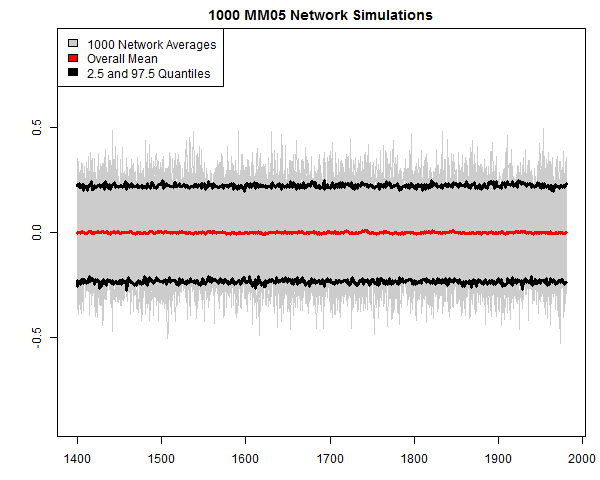
Figure 1. 1000 simulations using MM05 script. Grey- average for each network; red – overall average; black – 97.5 and 2. quantiles by year.
Mann’s Simulations Also Used Empirical Coefficients
But before ClimateBallers get too excited about our calculation of noise parameters from the empirical NOAMER network without first removing a “signal” that is not only unknown but the end-product of the calculation, they should first recognize that Mann also estimated noise parameters from the empirical NOAMER network (without such prior removal) in an important calculation.
In December 2004, in one of the earliest Realclimate pages (here), Mann reported the results of simulations using red noise series of the “same lag-one autocorrelation structure as the actual ITRDB data”:
Shown also is the null distribution based on Monte Carlo simulations with 70 independent red noise series of the same length and same lag-one autocorrelation structure as the actual ITRDB data using the respective centering and normalization conventions (blue curve for MBH98 convention, red curve for MM convention). In the former case, 2 (or perhaps 3) eigenvalues are distinct from the noise eigenvalue continuum. In the latter case, 5 (or perhaps 6) eigenvalues are distinct from the noise eigenvalue continuum.
In other words, Mann estimated his red noise parameters directly from the tree ring network – the same supposed offence that the ClimateBallers accused us of – but, needless to say, the ClimateBallers do not mention this. Nor was this a trivial calculation on Mann’s part. This was the calculation in which he purported to mitigate his erroneous PC methodology by arguing for the use of 5 PCs in the AD1400 NOAMER, an increase which enabled him to increase stripbark bristlecone weight through the backdoor.
Did MBH98 Use His Empirical Preisendorfer Calculation?
By (perhaps inadvertently) drawing attention to Mann’s 2005 “Preisendorfer” calculation, ATTP has raised an issue that is highly relevant to Steyn’s allegations of fraud and which ought to be minutely examined by Steyn and others. Indeed, this is one of the issues on which discovery might turn up something interesting.
Prior to our 2004 submission to Nature, there wasn’t a shred of evidence that Mann had done a “Preisendorfer” calculation for tree ring networks, though there was evidence that he done such a calculation on temperature networks. In 2005, Mann produced source code showing the calculation on temperature networks, but produced no such code for tree ring networks, even in response to a request from a House Committee. My own present surmise is that Mann didn’t use a “Preisendorfer” calculation for tree ring networks in MBH98, but was driven to this calculation in order to mitigate problems arising in 2004 from our exposure of Mann’s defective principal components method. Supporting this surmise is the impossibility of reproducing the actual pattern of retained PCs in MBH98 using the “Preisendorfer” calculation first attested in 2004. I believe that Mann was scrambling in 2004 to figure out some way of trying to mitigate his erroneous PC method and that his “Preisendorfer” calculation for tree rings was first used in 2004, not 1998.
If I were in Steyn’s shoes, I would require meticulous disclosure of the original calculations, which are totally undocumented. I would also be surprised if such discovery requests yields documents showing that Mann actually used the Preisendorfer Rule for PC retention in tree ring networks in MBH98.


112 Comments
If you ever get an intern (and I wish I could volunteer), it would be interesting to compile a list of Mann’s pronouncements on and defences of his work over the past 15 years. Failing that, I would urge Steyn’s counsel to look at the record.
If I understand correctly, his latest presentation in front of a crowd that actually included skeptics was bland and devoid of substance. He was not always so cautious.
As usual, you have done far more than yeoman work here. I don’t get ATTP in China so I can’t look at what they’re saying, but at least until Mr. Stokes shows up with his usual distractions it would seem that you have laid another series of questions to rest.
I think the suspicions are understandable. The thing is, hosking.sim is the blackest of boxes. You put in the data vec, you get back one simulated vec. No further information about what acf it calculated, the arfima, nothing. And there is virtually no documentation except for Hosking’s 1984 paper. Hosking didn’t write the code.
However, my view is one that probably no-one will cheer. I think this whole PC1 issue is misunderstood. Brandon says it is due to persistence. My analysis says the contrary. With white noise, the covariance matrix is just the unit, and every vector is an eigenvector. With short centering (last M=79 of N, N=581 etc), two eigenvalues change. One goes to N/M, the other to 0. Everything else stays 1. The eigenvector u corresponding to N/M is 1 for 1:(N-M-1), .5 for N-M, 0 for (N-M+1):N (to be normalised). So first myth bust – short centering does not enhance the HS. It sends it to zero in PC1. You can see it in the tableaux. In each HS-like case, the curve actually goes to zero at the ends.
Jean S: White noise?!? You really are either seriously challenged or you are doing this on purpose. There is no other plausable explenations. How many times it needs to be explained that PCs (real or Mannian) are nothing put orthogonal projections of the original data? It is extremely unlikely to find an orthogonal projection of 70 independent white noise series creating any significant “hockey stick”. If you’ve spent a half of a course in elementary statistics course you would know that. So you can stick all those white noise simulations of yours to the place where even the sun down under is not shining.
How many times it needs to be explained to you that the purpose of PCA is decompose the original data set such that the important “signals”, common to the data set are “summarized” in the very first PCs? How many times it needs to be explained to you that neither real or Mannian PCA is “creating” something out of thin air? How many times it needs to be explained to you that the issue here is that Mannian PCA is picking an “unimportant” (not common in the data set) and putting it to the first PC as long as the pattern resembles “hockey stick”?
Finally, it is obvious to me that you don’t even really even understand workings of PCA. We have here people who worked on PCA probably before even I was born. I did years ago part of my PhD work in PCA. Still, you come up with these crazy ideas starting that “your view is something that no-one will cheer”, i.e., you are going against all the experts here. Are you really suggesting that other people here are in some mystery conspiracy against you, or is that just arrogance of Mannian extend from your part? Do you really think that your BS here helps your “cause” or whatever it is you are doing it for? Think about it.
Last few days I’ve released quite a big portion of your sad commentary from the moderation. Since you don’t learn anything, from now on I won’t do it, and let Steve completely decide what portion of your spam is worth publishing here.
Second thing; nothing much has changed. u was also an eigenvector of the centered white noise. All that has happened is that some other bases are now excluded. The new set of bases are just a subset of the previous, which were all equally valid..
Third – this is virtually independent of persistence. That just changes the correlation matrix from I to something still diagonally dominant, and just smears out the eigenvector a bit. You can see this in the NAS AR1(.9) eigenvector (red) shown by Steve in the O’Neill thread. It is still that basic step function, just rounded a bit. The characteristic time for AR1(.9) is about 19 years (very long). That is still fairly short relative to the 79 years of the step function.
Fourth – none of this matters. It makes PC1 look funny, but has no effect when you actually use the basis for a recon, unless you use only PC1.
Jean S,
“Finally, it is obvious to me that you don’t even really even understand workings of PCA. “
I actually do. But you might like to explain with all this expertise how it happens that none of this hockey stick mining is reflected in the MM05EE reconstructions, when compared with MBH.
There is a useful observation there. It’s true that as the noise becomes whiter, the noise in PC1 (which depends on proxy numbers) grows and the HS jump becomes less visible. But the eigenvector of the covariance matrix that determines its shape is fairly invariant. That means that you aren’t expecting changes to turn up in other places. It’s somewhat supportive of Steve here. It doesn’t help if the hosking.sim is introducing signal, but it does mean that the mixed noise structure probably isn’t doing anything unusual.
You can try that. I’ve been playing with the NAS code that generated the Fig 9.2 that Steve showed. You can put any reasonable parameter into the AR1 model, and the correlation eigenvector barely changes.
nick
Its pretty clear your original complaint “The thing is, hosking.sim is the blackest of boxes. You put in the data vec, you get back one simulated vec. No further information about what acf it calculated, the arfima, nothing. And there is virtually no documentation except for Hosking’s 1984 paper. Hosking didn’t write the code.”is a red herring. There are cites available, books available…the code is available, there is a manual available, it seems like the only reason you didnt find these is that you didnt really look for them.
This is typical Nick.
Now you think he’s be smart enough having worked in R to KNOW that you CANNOT PHYSICALLY PUBLISH an R package to CRAN WITHOUT supplying all the source.
So he just MADE SHIT UP or lied when he called it a black box
Argument from ignorance it seems.
Who determined that 19 years persistence should be classified “very long” in the context of strip bark bristlecone pines? Where are your calculations or supporting evidence? Or does it come from the “black box” of you making completely arbitrary claims without any justification whatsoever?
Spence_UK sensibly observes:
Tree ring chronologies are (to a close approximation) averages of ring widths at a given site, after an allowance for juvenile growth. During the Climate Audit initiative to examine the Almagre strip bark bristlecones, Pete Holzmann located many of the trees actually sampled by Graybill. See tag “almagre” and, for example, here here.
One of the most important discoveries was that cores only several inches apart could have observations that were locally correlated but differing by more than 6 sigma, as for example, below. This phenomenon requires a very complicated error model to describe and no such model exists in the specialist literature. How do you define “noise” to accommodate the astonishing differences in ring width only a few inches apart? Nor are these problems necessarily random. Graybill’s original sample searched for stripbark trees. Red and black below show the widths of two cores only several inches apart.
Our diagnosis was that the “noise” in this case resulted from mechanical deformation of the tree. However, it appears that the “persistence” of the deformation can last even a couple of centuries. Obviously stripbark bristlecones are not cherrypicked examples to make Stokes look bad, but have been at the core of disputes over Mannian reconstructions since the beginning. If one actually looks at the persistence properties of strip bark bristlecones, 19 years is a ludicrous underestimate.
Pete Holzmann’s belief is that heavy snow can lead to strip bark (by tearing off boughs). On this scenario, the high incidence of mid-19th century strip barking might originate from (documented) very severe winters in the 1840s, but the resulting growth pulse be unrelated to temperature.
I notice those charts go beyond 2000. Is this your sampling?
Steve: Pete’s
“The thing is, hosking.sim is the blackest of boxes. You put in the data vec, you get back one simulated vec. No further information about what acf it calculated, the arfima, nothing. And there is virtually no documentation except for Hosking’s 1984 paper.”
Stop with the lying Nick. The package is in R. The source is there.
#include
#include
void hosking(double *Xt, int *N, double *vin)
{
int i, j, t;
int nrl = 1, nrh = *N-1, ncl = 1, nch = *N-1;
int nrow=nrh-nrl+1,ncol=nch-ncl+1;
double *vt, *mt, *Nt, *Dt, *rhot;
double **phi; /* = dmatrix(1, *N-1, 1, *N-1); */
vt = (double *) malloc((size_t) ((*N + 2) * sizeof(double)));
mt = (double *) malloc((size_t) ((*N + 2) * sizeof(double)));
Nt = (double *) malloc((size_t) ((*N + 2) * sizeof(double)));
Dt = (double *) malloc((size_t) ((*N + 2) * sizeof(double)));
rhot = (double *) malloc((size_t) ((*N + 2) * sizeof(double)));
/*** Begin dmatrix code ***/
/* allocate pointers to rows */
phi=(double **) malloc((size_t)((nrow+1)*sizeof(double*)));
/* if (!phi) nrerror(“allocation failure 1 in matrix()”); */
phi += 1;
phi -= nrl;
/* allocate rows and set pointers to them */
phi[nrl]=(double *) malloc((size_t)((nrow*ncol+1)*sizeof(double)));
/* if (!phi[nrl]) nrerror(“allocation failure 2 in matrix()”); */
phi[nrl] += 1;
phi[nrl] -= ncl;
for(i=nrl+1;i<=nrh;i++) phi[i]=phi[i-1]+ncol;
/*** End dmatrix code ***/
for(i = 1; i <= *N-1; i++)
for(j = 1; j <= *N-1; j++)
phi[i][j] = 0.0;
vt[0] = vin[0];
Nt[0] = 0.0; Dt[0] = 1.0;
Xt[0] *= sqrt(vt[0]);
rhot[0] = 1.0;
/* phi[1][1] = d / (1.0 – d); */
for(t = 1; t 1)
for(j = 1; j <= t-1; j++)
Nt[t] -= phi[t-1][j] * rhot[t-j];
Dt[t] = Dt[t-1] – (Nt[t-1] * Nt[t-1]) / Dt[t-1];
phi[t][t] = Nt[t] / Dt[t];
for(j = 1; j <= t-1; j++)
phi[t][j] = phi[t-1][j] – phi[t][t] * phi[t-1][t-j];
}
for(t = 1; t <= *N-1; t++) {
mt[t] = 0.0;
for(j = 1; j <= t; j++)
mt[t] += phi[t][j] * Xt[t-j];
vt[t] = (1.0 – phi[t][t] * phi[t][t]) * vt[t-1];
Xt[t] = Xt[t] * sqrt(vt[t]) + mt[t];
}
free((char*) (vt));
free((char*) (mt));
free((char*) (Nt));
free((char*) (Dt));
free((char*) (rhot));
free((char*) (phi[1]));
free((char*) (phi));
}
OK, Steve,
so what does it do?
I said it wasn’t documented. In fact I asked for hosking.sim. I’m in the environment, running the package, and it says:
> hosking
Error: object ‘hosking’ not found
> hosking.sim
function (n, acvs)
{
.C(“hosking”, tseries = rnorm(n), as.integer(n), as.double(acvs[1:n]),
PACKAGE = “waveslim”)$tseries
}
>
Looks dark to me. But anyway, what I said was that it lacked documentation. This isn’t documentation. Again, what does it do?
No nick so said it was a black box. It’s a white box.
What it does is obvious. Read the code
Oh and thanks for saying what I predicted you would say.
If the code doesn’t make sense to you then no explanation will help you because you will say that the explanation is dark.
You’re a liar
Steven, the suspicion is that the output carries some of the input signal. I’m not myself bothered by that. But I don’t see how you can expect to allay it by waving mostly uncommented C or R code and saying it’s obvious. Somebody needs to explain in English what the operation actually does.
So black box means it is a function written in C which no one via a google search has explained what it does?
Lack of documentation doesn’t mean it is impossible to figure out.
“Error: object ‘hosking’ not found
> hosking.sim
function (n, acvs)
{
.C(“hosking”, tseries = rnorm(n), as.integer(n), as.double(acvs[1:n]),
PACKAGE = “waveslim”)$tseries
}”
you MORON do you understand that this means the code is in C not R.
your incompetence is astounding. Turn in your keyboard.
typing in a function name hoskin.sim will return the R code associated with the function call.
This R code is
“.C(“hosking”, tseries = rnorm(n), as.integer(n), as.double(acvs[1:n]),
PACKAGE = “waveslim”)$tseries”
Anyone who knows R knows that to call a library written in starts with .C
incompetent boob
MattK
Nick is either stupid or playing dumb.
The first thing I did was load the package waveslim.
then type in the commmand hosking.sim
This returns the R code associated with the function. That R code shows a call to C
So, you have to open the source package that comes with every R package. you cant publish R without this.
He knows this
When you open the source package there is a subdirectory called src
the src subdirectory contains all the code that is not in R ( could be open source C, C++, fortran)
For example, nick has used svd in the past under R. svd calls FORTRAN libraries. he has never
once complained that svd is a black box, never once looked at that source or complained that there wasnt documentation.
So, he is either incompetent ( doesnt understand R ) or is just playing one of his misleading deceptive climateball games
Nick
“Looks dark to me. But anyway, what I said was that it lacked documentation. This isn’t documentation. Again, what does it do?”
It look DARK ( not black) to you ( nice moving of the goalposts climateballer) because YOU dont understand
R.
Its a call to C.
That TELLS any competent R programmer that the source for the function is in the “src” subdirectory of the package source.
Further, the Manaul points you the published literature explaining the function if you want that.
So the documentation is there you just refuse to get it. IF you wannt to understand, start with the code.
Its there. Its always been there but you are too stupid to even understand how R packages are built.
THEN if the code is not enough, go to the literature.
IF the literature is not enough, then email the maintainer or author. you cant publish R without it.
You have doubts about what it does. read the code.
Still stumped? read the book.
Still stumped, write the author
But dont expect us to waste our time explaining it to you when YOu can even understand the output that should have sent you to the “src” directory. Dope.
Steven,
Whether I know or don’t know my way around the R package system isn’t important. I’m not actually the one with doubts. All I’m saying is that it’s legitimate for people to wonder exactly what properties of the simulated series is retained from the data series fed in. And if no-one can explain in words just what the package is doing, and it seems no-one here can, then I think those doubts are understandable.
“Steven,
Whether I know or don’t know my way around the R package system isn’t important.
1. You complained it was a black box. You are wrong. Rather than admit that, you try to
fool people by showing your incompetence with R.
2. Then, you complained that it was a dark box because there was no documentation.
3. When the documentation ( 2 papers and book) was shown to you, rather than get the documentation
you doubted that it would help.
4. It is important because it goes to your credibility, your trustworthiness.
5. If you cant admit a simple mistake ( I was wrong to call it a black box), Then NO ONE here
has a reasonable expectation that you will admit a more difficult to find mistake.
I’m not actually the one with doubts.
1. You doubted that the book would illuminate the code.
2. you doubted that the function put out all the data needed to assess it.
All I’m saying is that it’s legitimate for people to wonder exactly what properties of the simulated series is retained from the data series fed in.
1. No, that is not ALL you are saying. You said it was a black box, then a dark box, then you
said R threw an error,
And if no-one can explain in words just what the package is doing, and it seems no-one here can, then I think those doubts are understandable.
The package is doing the following:
“Uses exact time-domain method from Hosking (1984) to generate a simulated time series from a specified autocovariance sequence.”
If you NEED or want an explanation of that you have these choices
1. Read the papers.
2. write the maintainer
3. Run the sample code
4. read the code.
What dont have the right to do is to ask people here to DO YOUR HOMEWORK.
Why would I do the homework for a student who
1. Cant understand R
2. Cant admit a mistake about calling something a black box
3. Doubts a book he never read
4. Doubts papers he never read
Pity. Nick had such a lovely rabble roused.
Re: Preisendorfer
Addition to the three cases that I showed it was impossible that any kind of objective criterion was used, we have to remember that in AD1000 step (i.e. MBH99) they selected 3 PCs as 2 was used in AD1400 step. Further, it is kind of impossible to understand how a “key pattern of variability” (in MBH98) collected into NOAMER PC1 suddenly becomes something that needs “fixing” when the only differences is that there are fewer proxies going into Mannian PCA.
“Third – this is virtually independent of persistence. “
OK, that was a bit rash. Persistence obviously changes the effect relative to the noise. But it doesn’t change the shape of the underlying eigenvector very much.
Nick:
A bit of vetting for this paragraph:
The source code for hosking.sim is available and there are multiple references (but a single one would suffice).
You have a “black box” source code when you can’t see the contents or know how it functions. Certainly a single reference that defines the method used makes the code not black box. Having access to the source also makes it not black box.
So not black box.
Anyway, there are two references listed plus a book:
Hosking, J. R. M. (1984) Modeling persistence in hydrological time series using fractional differencing, Water Resources Research, 20, No. 12, 1898-1908.
Percival, D. B. (1992) Simulating Gaussian random processes with specified spectra, Computing Science and Statistics, 22, 534-538.
Click to access Interface-92-all.pdf
Gençay, Selçuk and Whitcher (2001)
Link to the manual.
Brandon Whitcher is listed as the author of the package waveslim.
Nick will have to explain the importance of Hosking putatively not writing the original code in “hosking.c” from waveslim.
Carrick,
There is virtually no documentation with the R package. I wonder who has delved into the C source to figure it out?
Nick
Now your claim is no longer that the function is black box, just that no-one has bothered looking inside it.
When presented with a perfect opportunity to say you have learned soemthing new (in this case the presence of the book), and to correct a statement you have made, you change the argument.
Do you know if the book is helpful?
Do you? No, you changed the question
Nick,
Umm…It’s a 2 kilobyte source file Nick,and at first glance looks not very complicated. So, not much to delve into. Is the issue that you don’t know C, or something else?
Seems to me that at bottom (despite of all the discussion of who understands how PCA works, the right number of PC’s, centering, and the rest), the issue being contended is something pretty simple: What is a realistic noise model for trendless (synthetic) proxy series? If the noise model has long persistence, then PCA will find almost always find series which match any target pattern, including a hockey stick, and scale them to be “important” in the reconstruction. If the persistence is short, then PCA will find only a very poor match for any target series, including a hockey stick. Do you agree? How do YOU think a realistic noise model should be determined?
Steve,
I haven’t made an issue of the noise model. I just noted that there is little documentation of hosking.sim, and I don’t think C source code really qualifies. Maybe the book helps – I don’t know. And there is no useful numerical output apart from the bare synthetic series.
I agree that the method will, with persistence, ensure that a HS-like vector will tend to be part of the basis set. That doesn’t need to imply importance. The key issue with PCA is truncation. If you retain enough PC’s to represent the non-hockey behaviour, that will then sort itself out. As it seems to have done. Again I come back to it – look at the results.
forgive this interruption, but do you get to assign a persistence coefficient when you generate red noise? When you generate red noise, is the product a stream that you cut off when you have enough, or is it qualitatively different if you give it a finite length (number of points)? Since the paleo-data looks like a time-series to me, are the red noise ‘episodes’ constructed with a known number of increments – ie. number of days between 1400-2000?
The follow on question if you do choose persistence will be can you code running the generator with varying persistence to see when the hockey sticks crop up? And while we’re at it, I assume that the association of paleo-data with red noise can be done by analysis – doesn’t just depend on “It sure looks like red noise to me.”
It’s ok to tell me to go back to school and learn this stuff for myself.
Given that source code, I think it qualifies very well as documentation. Given your linear algebra knowledge, I doubt you would have trouble making sense of:
 vt[0] = vin[0];  Nt[0] = 0.0; Dt[0] = 1.0;  Xt[0] *= sqrt(vt[0]);  rhot[0] = 1.0;

  /* phi[1][1] = d / (1.0 - d); */
for(t = 1; t 1)
for(j = 1; j <= t-1; j++)
Nt[t] -= phi[t-1][j] * rhot[t-j];
Dt[t] = Dt[t-1] - (Nt[t-1] * Nt[t-1]) / Dt[t-1];
phi[t][t] = Nt[t] / Dt[t];
for(j = 1; j <= t-1; j++)
phi[t][j] = phi[t-1][j] - phi[t][t] * phi[t-1][t-j];
}
for(t = 1; t <= *N-1; t++) {
mt[t] = 0.0;
for(j = 1; j <= t; j++)
mt[t] += phi[t][j] * Xt[t-j];
vt[t] = (1.0 - phi[t][t] * phi[t][t]) * vt[t-1];
Xt[t] = Xt[t] * sqrt(vt[t]) + mt[t];
}
Nick,
The problem with letting it all sort itself out is that you don’t know (and I think can’t know) how much the red noise contribution to the reconstruction leads to ‘statistical validation’. I mean, the target series is just a hockey stick; if red noise gives you a “validated hockey stick”, then what can you really say about how much real temperature contribution there is? Now if you validated based on only part of the temperature data and then compared the reconstruction to other part of the temperature data, you could reasonably argue that the reconstruction is valid. But I am guessing that the reconstruction is too noisy to be able to do that kind of validation (I could be mistaken though).
John F.
The red (or pink) noise series can be generated lots of ways (spreadsheet or most any programming language). The trend “evolves” because each successive value is partially due to the previous value in the the series plus some “white noise” influence (and since the previous value was linked to the value before that, the influence of the past extends backward in the series for some distance). How “red” or persistent the series is depends on what fraction for each successive value comes from the previous value. 1%? 10%? 50%? 90%? A constant like 0.5 means half is from the past and half is white noise; the influence of previous points declines as 0.5, 0.25, 0.125, 0.0625, etc. While a larger value (like 0.9) declines much more slowly. The bigger the constant (closer to 1.0)the more slow wander in the trend values you see in the series, and the more likely you will find most any specified target shape in the series (eg hockey sticks). Hope that helps.
Nick,
First you claim it is a black box. You were wrong.
Now you say that there isnt any documentation.
The CODE is the perfect documentation. It shows you exactly what is done and how.
If you want different output, modify the code and recompile.
do that before you post another post and tell more lies.
trust me MikeN the code provided is way more clear than code that Nick has provided.
Waay more clear
Indeed, Nick. Unless McIntyre has produced a formal proof of the correctness of these 50 lines of C code his reliance on them once again demonstrates a hopelessly amateur approach to things.
Also, I believe that he sometimes neglects to be *completely* thorough when recycling household garbage, and apparently his favorite recreation is vivisecting juvenile ocelots, which he performs clumsily.
Unlike Mann’s code for confidence limites, Steve’s code has been available since the paper was published. The routine you are complaining of has 23 lines of code and they are visible in comments here. Do you have a real complaint or are you just slinging mud?
Proof that it is always worth making it through to the last paragraph before commenting on a post 🙂
void hosking(double *Xt, int *N, double *vin)
{
int i, j, t;
int nrl = 1, nrh = *N-1, ncl = 1, nch = *N-1;
int nrow=nrh-nrl+1,ncol=nch-ncl+1;
double *vt, *mt, *Nt, *Dt, *rhot;
double **phi; /* = dmatrix(1, *N-1, 1, *N-1); */
vt = (double *) malloc((size_t) ((*N + 2) * sizeof(double)));
mt = (double *) malloc((size_t) ((*N + 2) * sizeof(double)));
Nt = (double *) malloc((size_t) ((*N + 2) * sizeof(double)));
Dt = (double *) malloc((size_t) ((*N + 2) * sizeof(double)));
rhot = (double *) malloc((size_t) ((*N + 2) * sizeof(double)));
/*** Begin dmatrix code ***/
/* allocate pointers to rows */
phi=(double **) malloc((size_t)((nrow+1)*sizeof(double*)));
/* if (!phi) nrerror(“allocation failure 1 in matrix()”); */
phi += 1;
phi -= nrl;
/* allocate rows and set pointers to them */
phi[nrl]=(double *) malloc((size_t)((nrow*ncol+1)*sizeof(double)));
/* if (!phi[nrl]) nrerror(“allocation failure 2 in matrix()”); */
phi[nrl] += 1;
phi[nrl] -= ncl;
for(i=nrl+1;i<=nrh;i++) phi[i]=phi[i-1]+ncol;
/*** End dmatrix code ***/
for(i = 1; i <= *N-1; i++)
for(j = 1; j <= *N-1; j++)
phi[i][j] = 0.0;
vt[0] = vin[0];
Nt[0] = 0.0; Dt[0] = 1.0;
Xt[0] *= sqrt(vt[0]);
rhot[0] = 1.0;
/* phi[1][1] = d / (1.0 – d); */
for(t = 1; t 1)
for(j = 1; j <= t-1; j++)
Nt[t] -= phi[t-1][j] * rhot[t-j];
Dt[t] = Dt[t-1] – (Nt[t-1] * Nt[t-1]) / Dt[t-1];
phi[t][t] = Nt[t] / Dt[t];
for(j = 1; j <= t-1; j++)
phi[t][j] = phi[t-1][j] – phi[t][t] * phi[t-1][t-j];
}
for(t = 1; t <= *N-1; t++) {
mt[t] = 0.0;
for(j = 1; j <= t; j++)
mt[t] += phi[t][j] * Xt[t-j];
vt[t] = (1.0 – phi[t][t] * phi[t][t]) * vt[t-1];
Xt[t] = Xt[t] * sqrt(vt[t]) + mt[t];
}
free((char*) (vt));
free((char*) (mt));
free((char*) (Nt));
free((char*) (Dt));
free((char*) (rhot));
free((char*) (phi[1]));
free((char*) (phi));
}
omg it’s all so clear now, practically a bestseller.
Jean S says PCA finds hockey sticks. Decentered or centered.
Wellwell. Finally.
What was the problem? Some strange idea that only PC1 can say anything about the data?
Utterly strange.
Jean S: Things might appear less strange if you’d have actually understood what I’ve written.
Ever wondered why PC1 is called PC”1″?
(Humour).
“ClimateBallers have additionally expressed concern, not always politely, that the supposed “trendless red noise” of MM05 had somehow surreptitiously imported HS patterns and that the MM05 histograms and related results were an artifact of these imported patterns, a claim sometimes asserted with considerable conviction.”
……….
Steve, play some of it backwards to see if the residuals have a sinister message – or not.
Sent from my BlackBerry 10 smartphone. From: Climate AuditSent: Tuesday, September 30, 2014 12:47 AMTo: hswiseman@comcast.netReply To: Climate AuditSubject: [New post] ClimateBallers and the MM05 Simulations
a:hover { color: red; } a { text-decoration: none; color: #0088cc; } a.primaryactionlink:link, a.primaryactionlink:visited { background-color: #2585B2; color: #fff; } a.primaryactionlink:hover, a.primaryactionlink:active { background-color: #11729E !important; color: #fff !important; }
/* @media only screen and (max-device-width: 480px) { .post { min-width: 700px !important; } } */ WordPress.com
Steve McIntyre posted: “ClimateBallers are extremely suspicious of the MM05 simulation methodology, to say the least. A recurrent contention is that we should have removed the climate “signal” from the NOAMER tree ring network before calculating parameters for our red noise sim”
Happy to see Jean S wouldn’t mind using more than PC’s in recontructions. So what is the problem?
I know: Try to divert attention from MM’s cherrypicking. Smokescreen indeed.
OK. It’s quite obvious that you do not like Steve, but what other useful information or contribution do you think you can offer to the discussion?
Apparently ehac is simply regurgitating talking points without first bothering to read the post.
Please explain what you mean by MM Cherrypicking.
In an earlier thread Steve responded to a point about selecting by HSI as follows:
when he says “most figures” are based on high-HSI values, I presume that he means Wegman Figure 4.4, a figure that was produced long after our articles had received considerable publicity and which attracted negligible contemporary attention. The relevant MM05 figure, Figure 2, is based on all 10,000 simulations. I haven’t gotten to a discussion of Wegman Figure 4.4 yet, as I wanted to first clear up issues about orientation and the “hockey stick index”, which ClimateBallers use to move the pea, but I do plan to discuss it.
My thanks to Jean S and Steve for the detail provided in these recent posts. I have enough of a background in statistics that I can follow the arguments here but rarely have enough knowledge to even consider commenting. Nonetheless, I want to comment that the results of this work disappoints me. I check out Watts up with That and this site on a daily basis in no small part because I have had this naïve belief that there could be an analysis that would prove beyond all doubt that the science used to justify the politically correct response that without an 80% reduction of emissions by 2050 that catastrophe is inevitable. The responses to these analyses suggest to me that advocates cannot be convinced to change their views however detailed the dismantling of their “proof”. Thank you for trying.
Your comment reveals that you have no clue what Steve believes or why he maintains this site. Over years of following this site nearly daily, I have never read anything by Steve remotely denying that climate is changing or that global temperatures are trending warmer. However, Steve has vigorously challenged sloppy, misleading, hyperbolic and defective advocacy motivated science.
snip/Jean S: Please, do not continue with the “general picture” (blog policy). This post is about MM05 simulations.
ClimateBallers are suspicious of *the results* of MM05 methodology, which demonstrates convincingly that they are wrong; to ClimateBallers such a result must be prohibited at all costs, therefore any cavil, no matter how petty or unnecessary, becomes an imperative.
Proving a case where “McIntyre goofed” seems to be the obsessive [and ever elusive] Holy Grail of the Baller sub-culture.
Of course, I could be wrong about all of this.
W^3
Nick Stokes says:
Based on what? You have cast aspersions but provided no evidence to support that. If you have reason to doubt the validity of the algorithm either:
(a) Show the original paper is wrong in some material way
(b) Show the implementation in the source code is wrong in some way
(c) Show that the algorithm fails some reasonable statistical test that you pose
Otherwise you are simply blowing hot air.
Not really. As others note here, the source code is available online. It only runs to 48 lines/b> of C code, of which 6 lines are declarations, 7 lines are setup and 12 lines are memory allocation/deallocation ie housekeeping. That leaves just 23 lines of source code for the algorithm. There’s not a lot too it and its hardly a black box when you can read the source code and reference the original paper n the implemenio paper. Or maybe you can’t? Still you are in good company, as it seems Eugene Wahl struggled with hosking.sim too…see:
http://r.789695.n4.nabble.com/Use-of-hosking-sim-R-function-td799138.html
As for the supposed introduction of hockeysticks or some such by using hosking.sim, that algorithm is clearly designed to “Generate Stationary Gaussian Process Using Hosking’s Method”. Sounds like it pretty much does what it says on the tin and Steve’s plot above demonstrates that pretty convincingly.
Unless, of course, you know different Nick? In which case provide some evidence. In the meantime, have you stopped beating your wife, Nick?
I’m pretty sure MBH tree ring PC selection plus MBH99 confidence limits are an even blacker box, since we don’t have source code, and the limited descriptions we have are discordant with what was actually applied. Wonder what Nick’s view is on that?
The box with intelligible open code is black, the spectacles admiring the fifteen-year-old one with no code rose-tinted.
TS,
OK, so do you know what it does?
Spence,
“Wonder what Nick’s view is on that?”
What’s your view?
I’m actually not suspicious myself – because I don’t think the noise model changes that much. That’s why I suggest, correctly, that no-one would cheer. But I actually had in mind there, the folks with suspicions.
I went looking for discussion, anything, on what hosking.sim actually did, and found very little. My black box reference was to the functionality of the code. You put a data vec in, you get a simulation out. Most R packages give you some sort of structure that you can query to find out ahat it did.
That doesn’t seem to merit much discussion. You can tell what it does by looking at the source code.
“My black box reference was to the functionality of the code. You put a data vec in, you get a simulation out. Most R packages give you some sort of structure that you can query to find out ahat it did.”
WRONG. a great number of R programs are written on top of estblished libraries in C or Fortran.
go ahead, type in svd at the console, dope.
want to understand, start with one of the papers the programmer pointed you at
Click to access Interface-92-all.pdf
definition of black box
http://en.wikipedia.org/wiki/Black_box
The source is open. its on R Forge and in the “src” subdirectory
Clear box.
undocumented?
nope, papers pointed to. RTFM.
He didn’t say it was ablack box, he said the blackest of black boxes.
Yes I do know what does. It generates a stationary Gaussian process using Hoskings method. SM plot in this post suggests the realizations are stationary to second order at least.
But if you think there is a problem with the algorithm, go ahead and demonstrate it, if you can.
Steve, Have you thought of using the HSI, or the t statistic, as a means of comparing the 70 tree ring series in the NOAMER network to the series you generate in the simulation. Presumably, you could look at how the HSI is distributed among the 70 NOAMER series compared to the distribution in your simulated series. I know 70 is not that large a sample size, but something informative might come out.
Karl asked:
Good question and one worth revisiting using the t-stat. I had previously allocated the 415 MBH98 proxies into 9 proxy types, keeping bristlecones as a separate class. I calculated the tstat for the difference between the blade period (1902-1980) and shaft period (start-1901) for all 415 series.
From 415 series, 24 had tstats greater than 1. 14 of 29 stripbark bristlecones had +1 tstats, as opposed to 10 of 386 for the balance. Interestingly, none of the 13 instrumental series had positive tstats – a couple had negative tstats. Within the MBH98 NOAMER network, the only +1 tstat tree ring chronology that was not in the Graybill stripbark (bristlecone, foxtail) group was Gaspe. The other North American tree ring chronologies with +1 tstat were in the Jacoby group. Jacoby was also responsible for the only Asian tree ring chronology with a +1 tstat.
First column below is number of series, 2nd is number of +1 tstat.
Proxy Count +1-tstat
bristle 29 14
coral 9 0
guage 11 0
ice 9 2
instrumental 13 0
tree_ASIA 67 1
tree_AUSTRAL 18 0
tree_EUROPE 10 0
tree_NOAMER 236 6
tree_SOAMER 13 1
Corrections:
moderator – missed a “. Wireless keyboards!
Line should read “original paper and the implementation paper.”
Why is red noise being used? Is it because the tree rings themselves exhibit such a pattern, which is not intuitive?
Red noise is time correlated whereas white noise is not.
Reading the comment by ATTP that SM quotes:
It seems to me that ATTP and many others fail to understand (either wilfully or not) the difference between the stationary random process being simulated and the individual realisations of that process. If the random process has persistence then it will have “trends” of some description in some realisations, perhaps at the beginning, the end, the middle and so forth. That is the nature of stochastic simulations with persistence (or spatial or temporal correlation, or however else you want to describe it). “Trendless” refers to the stochastic process, not the individual realisations. The mean of the realisations will be trendless. SM shows this clearly in the Figure accompanying this article.
As MM2005_GRL clearly state:
And it was that paper, with its “money shot” Figure 2 that clinched the whole argument for me: conventional calculation, centred histogram; MBH98 calculation, hockey sticks from trendless random noise.
How anybody can not get it is beyond me and quite frankly they must be beyond help. I doubt it even matters what method of simulation is used, if the realisations have persistence and are from a trendless, stationary stochastic process, the results of Figure 2 from MM2005_GRL would still stand.
PS Link to MM2003 on sidebar appears to be broken.
“A couple of responses. First, if the strip bark growth pulse (as much as 6 sigma in some trees) is related to mechanical deformation (as Pete Holzmann, myself and seemingly Keith Briffa and Jan Esper believe), it is “noise” (not signal), but not noise that can be modeled as AR1, and, perhaps not even as arfima (though arfima is better at capturing some of the variability.) In some instances, there is elliptical deformation, with the growth pulse being a change from the short part of the ellipse to the long part. It seems to me that arfima is better than AR1 for this sort of problem, though even arfima has important shortcomings in the exercise. But be that as it may, the arfima networks show the existence of an important bias in Mannian principal components. In our 2005 articles, having established the existence of the bias, we turned our attention to its impacts.”
I hope that this paragraph from SteveM’s introduction to this thread is carefully read, understood and appreciated. The noise in the proxies comes in many shapes and forms and it cannot be ignored or over simplified when analyzing and determining the validity of temperature reconstructions. Admitting to the existence of these noises and dealing with the consequences by those doing reconstructions would be a huge first step in the right direction. It would put a spotlight on the basic error of selecting proxies ex post facto.
As SteveM points out one cannot start from the premise that all proxies can be simulated by assuming each is independently generated by random red noise. We know that some proxies of the same type and from the same region can manifest similar patterns and are thus not independently generated. Nevertheless we have good reasons to suspect that those patterns are generated by noise and are not a temperature signal.
If you plot these individual proxy series as I have done with all 1209 of the Mann 2008 proxies and now the 212 NA TR proxies from Mann 1998 and observe the patterns you could readily be led to seeing what one might expect from an ARFIMA model with long term persistence for some of the proxies. Some proxies will look like white noise and some like having various levels of red/white noise. Some of the series show secular trends on doing a singular spectrum analysis and those trends can be from long term persistence or generated by deterministic forces (and yet be noise). Those secular trends appear in random directions (up and down) and series locations.
I want to put together a simple minded analysis of the 212 proxies noted above to show the result of these effects noted here.
You Have CLimateBallers and WreckingBallers…
Perhaps a better name would be “Climatebawlers”.
SM: ClimateBallers are extremely suspicious of the MM05 simulation methodology, to say the least.
I think the words you are looking for are ‘Climate bloggers’ and ‘skeptical.’
Apologies to Skee-Lo…
I wish I was a little bit taller
I wish I was a climateballer
I wish I had a girl who looked good
I would call her
I wish I had a rabbit in a hat with a hockey stick
And a six four Impala
From a Quality Assurance auditing perspective in examining how the climate science community is conducting its temperature reconstruction research, and from the perspective of a legal need to determine just what kinds of information are relevant to the Mann-Steyn / Steyn-Mann series of lawsuits, I still have to ask a question for which no one has yet provided an answer:
THE QUESTION: What is the precise scope and extent of that body of climate science research which: (1) comprises “the Hockey Stick” as it now is being discussed here on this blog and on other blogs; and which (2) is the focus of the Mann-Steyn / Steyn-Mann series of lawsuits?
Why would anyone ask this very basic question? For one example of a reason, would it be possible for Michael Mann to argue that the latest Hockey Stick is much improved over the earlier versions that were produced in 1998 and 1999, so that these earlier versions are irrelevant to the issue of whether or not the Hockey Stick as it existed in the summer of 2012 is scientifically defensible?
To help put Nick’s suspicions in context, I would ask him (and other AGW advocates): How many times has Steve M made a mistake and not admitted it? How many times has he been intentionally deceptive? Please provide examples.
Next consider Michael Mann and Gavin Schmidt and ask the same questions. Then state your conclusion as to who has been the most straightforward person with respect to climate statistics and data.
Having gone through this exercise, we can all decide whether there is any legitimate reason to be suspicious of Steve M’s work. Of course, his work like that of anyone else should always be open to scrutiny. The question should be whether it is legitimate to question his work without having specific focused questions.
JD
Well now we understand Nick’s criteria.
If someone uses a piece of code, then its a black box and suspicious.
If the code is available, this doesnt make it less suspicious.
If they published a book, this may not help.
If it doesnt output exactly what he refuses to specify, then it’s still suspicious.
Nick has just rendered climate science suspicious.
Yes, and how often have the CimateBallers incl. Nick been suspicious of Mann & Co?
Nick has given us a whole new set of objections.
When mann uses some matlab we can now call the functions “black boxes”
When and if the code is produced the code is “not good documentation”
When a book is published, we can argue that it may or may not help with the
code, and besides, the function doesnt output everything we want.
He’s just handed folks a whole new set of climateball rulz.
You see in the beginning climateball was akin to Calvin Ball, where the rulz change
What better example of climateball is there than the Race Horse
The function is a black box ( a technical term which means you cant examine internals)
Show him the internals…and the rulz change.. The code isnt documentation
( yes documentation tells you what was done, code SHOWS you). Pointed at a book
of documentation, we get “The book might not help” If you showed the book
did help, he would argue “it doesnt help me, I want different output”.
Modify the code to give him different output and he would say
Well Hosking.sim really wasnt my point after all
ClimateBaller maximus
It’s a pity – I’ve appreciated some of Stokes’ work and I used to think the group-scragging of him which went on here & elsewhere as annoying & pathetic.
But over the last few days on these threads I think he’s blown away his credibility in a pretty amazing fashion, via lame content & embarrassingly low-rent rhetorical techniques.
Stokes is using the Vermeer rules. If the code is suspected to be written by a skeptic, then it is ugly and inscrutable. If not, then it is well written and obvious as to meaning.
http://arthur.shumwaysmith.com/life/content/michael_manns_errors
I must say that when trying to follow Nick’s reasoning I am sometimes reminded of a classical Orwell quotation:
“To know and not to know, to be conscious of complete truthfulness while telling carefully constructed lies, to hold simultaneously two opinions which cancelled out, knowing them to be contradictory and believing in both of them, to use logic against logic, to repudiate morality while laying claim to it, to believe that democracy was impossible and that the Party was the guardian of democracy, to forget, whatever it was necessary to forget, then to draw it back into memory again at the moment when it was needed, and then promptly to forget it again, and above all, to apply the same process to the process itself”
Nick is not paid to be logically consistent and well reasoned. He is paid to confuse the issues and sow doubt among those who can’t quite follow. At that, he is very good.
Many exhibit crimestop
The mind should develop a blind spot whenever a dangerous thought presented itself. The process should be automatic, instinctive. Crimestop, they called it in Newspeak.
He set to work to exercise himself in crimestop. He presented himself with propositions—’the Party says the earth is flat’, ‘the party says that ice is heavier than water’—and trained himself in not seeing or not understanding the arguments that contradicted them.”
“The faculty of stopping short, as though by instinct, at the threshold of any dangerous thought. It includes the power of not grasping analogies, of failing to perceive logical errors, of misunderstanding the simplest arguments if they are inimical to IngSoc, and of being bored or repelled by any train of thought which is capable of leading in a heretical direction. In short….protective stupidity.”
Sven,
Very good point.
JD
At the risk of making a point that is obvious, if a person implements an unconventional application of a well-known statistical tool, shouldn’t he be obligated to:
1) Disclose that he is using an unconventional application ;
2) Explain the statistical properties of the unconventional application;and
3) Explain why the unconventional application is more appropriate than the conventional application for the task at hand?
It amazes me that the climate science community can in good faith give Michael Mann a free pass on all the above, and then place the burden on SM to prove to their satisfaction that there are problems.
Steve, I have a question. Nick Stokes has a (in my opinion ridiculous) post up which uses an emulation of your MM05 Figure 1 (his emulation was posted . The version he posts has some difference though. Notably, his emulation begins at ~.175 whereas your begins at slightly over .2, and his ends at a higher point than yours. The effect is his emulation shows the most recent part of the reconstructed series is unprecendented whereas yours shows the first 30 years surpass it.
Do you know what causes this discrepancy? My assumption right now is it’s a matter of smoothing, but I’m not sure what smoothing would produce which results.
I’m also not sure why a graph Michael Mann created which you recently showed would be different.
I don’t think anything hinges on these differences, but it would be nice to know why the displays are different.
Steve: don’t know offhand. Our code reconciled to seven 9s exactness with Wahl and Ammann, so there should be exact matches between our graphics and WA if properly matched. It would probably be a good idea to repost some contemporary discussion of Wahl and Ammann, since Nick is fabricating this backstory. One of the reasons why our EE commentary so exactly anticipated Wahl and Ammann cases is that we commented on Mann’s submission to Nature, which raised the same main issues as Wahl and Ammann, who did not credit Mann for his prior raising of the issues in Wahl and Ammann – something that would normally regarded as serious plagiarism.
Hrm. I’ve plotted the data series from this file, and I get results about the same as those in Stokes’s figure. It’s mostly similar to what you showed in MM05EE, but there is definitely something different about the endpoints. I’ll try looking through your code to see what smoothing you used in the display.
Oh dear,
he’s showing MM EE (2005) Figure 1 (the full emulated recons), and then claiming
Stokes does not even understand the stepwise nature of the MBH procedure! No Nick, you got it upside down, the effect should be visible (and is) in the other end, where there are few proxies (and Mannian treering PCA gets in to it’s full strength, i.e. the pre-calib length is much longer than the calibration length). What a clown you are, Nick.
“No Nick, you got it upside down, the effect should be visible (and is) in the other end”
Well, <a href="”>here is the Ammann and Wahl emulation for the millennium. No sign of these ambidextrous hockeysticks there.
More disinformation from Stokes. Even Mann and Wahl-Ammann understood that the regression operations caused the effect at the beginning of the step, not the end. If Stokes worked through Mannian regression, he’d see why.
Steve McIntyre: “…who did not credit Mann for his prior raising…”
Mann?
Yes.
I don’t come here often, and now I remember why!
Not only is there a deep-seated, and slightly worrying, obsession with matters of history (as if it could possibly change anything in the here-and-now) but there is a nasty vein of unpleasant arrogance (some arrogance can be occasionally borne with a weary shake of the head if it’s well-intentioned and/or mostly unconscious) and nasty and self-satisfied vituperation.
You may not care, I suppose, and definitely won’t agree, but this site (and this thread in particular) is looking like a discussion between adolescents to see who can sound the most clever and who can come up with the most dismissive comment towards someone they feel superior towards. Seriously, look at the language you’re using: “ClimateBallers” (does that even mean anything to anyone who isn’t as obsessed as all of you seem to be here?), “your BS”, “he just MADE SHIT UP or lied” (just how old are you?!), “Argument from ignorance”, “What a clown you are”.
If Nick Stokes is trying to get you all to reveal your true natures and to show the psychological underpinning of so-called scepticism (simply by asking questions and remaining calm and reasonable), he is doing a great job!
And you wonder why the real world is crossing over the road to try to avoid having anything to do with you? (Apart from those who think they can help you and integrate you back into society, of course..!)
Anyway, carry on – it’s fascinating, in a car-crash horror sort of way. But you should really have a look at yourselves some time and see how you look to others. You might be surprised. Then again…
JFM — “Adolescents”
If you want to talk about adolescents, you may want to look at climate “scientists”, such as Mann, Trenberth and Hansen who use the ridiculous term “D..” to describe those who critically examine nascent climate “science.”
JD
While I’m still here, and not wanting to disrupt the adult discussion here any further, I have to say that your comment, JD, is not unexpected – ‘What about them, sir. They started it first and they’re worse.’ God…
Don’t hurt yourself reaching, they’re sour.
============
You might have a point if billions in government and private spending were not premised on the science they are discussing.
You are complaining about style and ignoring the substance. Either that or you don’t fully understand the significance of these issues.
I disagree that the matters of history could not possibly change anything in the here-and-now. The detailed dismantling of the Mann hockey stick is appropriate because it still keeps coming up as “proof”.
While I can see your point that this discussion is digressing I believe that is the because of the frustration that no amount of detailed enumeration of the flaws in the methodology seem to be able to convince certain individuals that the Mann hockey stick should be thrown away and never mentioned again because it is wrong.
“and see how you look to others”
To most people, they look honest and reasonable.
This is why the IPCC goes nowhere, why attempts at global emissions reductions have been a total failure, and why nobody believes most of the garbage coming out of climate science. The only people who push the propaganda are the people who want to use it as a vehicle for other political ambitions such as bigger government (which happens to be a lot of people, funny enough).
It is not hard to see how this looks to others. Just look at the polls (and no, I don’t mean that absurd excuse for a paper published by Cook and friends, I mean real polls of real people who are smart and have no skin in the game).
Oooh, a concern troll at CA.
And, before I go to bed…
I am not concerned, Matt – I am secretly pleased, especially now that you have added an extra layer to the obsession by classifying me as a ‘troll’ and increasing the bafflement of those in the real world by using the term ‘concern troll’.
This couldn’t really get more irrelevant, funny or bizarre.
Well, as long as everyone is happy and feels they make a contribution. To something.
Including yourself it appears. Why are you secretly pleased unless you have some bias already? Otherwise you wouldn’t be pleased to see such things.
I think it is a big mistake to totally derail a valuable thread like this one, on a nothing issue like why did Nick Stokes call something a black box. IMHO it’s a good candidate for snipping every one of these comments for being Off Topic.
“Steve McIntyre: If I were in Steyn’s shoes, I would require meticulous disclosure of the original calculations, which are totally undocumented. I would also be surprised if such discovery requests yields documents showing that Mann actually used the Preisendorfer Rule for PC retention in tree ring networks in MBH98.”
While I have no doubt of the merits of this idea, I also wonder whether such tactics would work in a court of law. Delving into such details goes beyond what a juror or judge can evaluate on his own. At that point, it simple becomes a matter of who to believe: the Nick Stokes and Michael Manns of the world or the majority of commenters on this page.
I am more inclined to believe that the simple pictures of the proxies from which the stick was derived, next to the stick itself, that would be easier to understand by those not conversant in proxies and statistics, such as what Schollenberger produced on his blog. Any intelligent person can understand the issue when looking at it that way.
Other simpler attacks might also be easier to understand. For instance, his recent mistake in which he claimed that he had no involvement in one of the published sticks, yet it is listed on his CV. Anyone can understand that it is hard to keep your story straight when you’ve been lying for a long time. Anyone can understand it is easy to remember if you’ve contributed to a published graph that is significant enough to put on your resume.
The third example that comes to mind is Mann’s own characterization of McIntyre and Mckitrick’s paper as fraud. No doubt that if the Mann himself can call someone else’s well-respected paper fraud, surely that disqualifies his own suit.
These simpler arguments strike me as more likely to succeed in a court of law. Of course, meticulous disclosure of the original calculations might be more harmful to Mann scientifically than legally, which is probably why he appears to be avoiding his day in court at all costs.
Steve: I entirely agree that simple CV things are easier to explain to jury. I also think that the case will stand or fall on Mann’s false claims about the “exonerations” – a line of reasoning that is emphasized in the new CEI brief – and that no one will be satisfied with the outcome. Nonetheless, there is something really odd about Mann’s principal components. I’ve got pretty good instincts on these things. If someone else thinks otherwise, so be it. It’s something that I think that would be more worthwhile to probe in discovery than topics which will result only in talking points.
Steve:
Without making promises, Steyn seems to be listening.
Depending on what is the most appealable point, NR’s brief may moot a look into exonerations.
I find the tone, level of frustration and outrage indicated here absolutely justified!
Michael Mann and the “Team”, and lately, Nick Stokes, have worked long and hard to earn the responses they have received here. If one has any depth of understanding as to the level of error and the scale of its consequences, a mere intellectual and academic response is actually insufficient, and has proved to be, continuously, since at least 2003.
Good night to the anonymous and infrequent JFM!
Long ago I developed and installed a 60 db N-S notch filter.
It has been interesting to read the comments and try to guess
what he has been up to. Ok, given a totally black box, an EE would
try to figure it out with a series of tests; delta function input
response, step function input response, various responses from
increasing the input frequency in steps. Knowing nothing about the
black box you can estimate what’s in there with a series of tests.
What really helps is to have the code and a book that explains it.
We went to the moon with Fortran………..C is just for spreadsheets.
I meant to comment on this sooner, but I’ve been involved in field work the last five days.
Steve McIntyre quotes ATTP as saying:
The issue here is not whether there are hockey sticks in the MBH data, but how many of these hockey sticks are associated with temperature variations. If most of them aren’t temperature related, this is a problem for an algorithm that over-weights hockey sticks.
While I think it is important to understand how McIntyre and McKitrick generated their Monte Carlo series, it is obvious to me at this point, that none McIntyre and McKitrick’s blogosphere critics actually understand how these series were generate
As I discussed on Brandon’s blog,
My concerns with what McIntyre and McKitrick have done is they may not have enough “non-temperature [hockey-stick-shaped] climate signals” rather than too many. By concerns, I mean “this is something I think needs to be checked” rather than “I think they probably got it wrong.”
Again, it is critical if you want to test the robustness of an reconstruction method that you replicate non-temperature-related temporal features in the Monte Carlo data set you wish to test the reconstruction against.
The concerns I mentioned in that quoted material about econometric models have to do with, ironically here, the black-box way that many people uncritically apply these models. Forcing oneself to step outside of mathematical machinery can help in properly characterizing the properties of the noise in the data set you are trying to model, even if you eventually select an econometrics approach to actually perform the final simulations.
While I’m at it, 19-years is an absurdly short period to assume for the persistence of noise in this type of data. I can believe you might get it from AR(1), but AR(1) is a completely awful model for this type of data.
Carrick, in our replies to COmments to Huybers and VOn Storch and Zorita, we did some analyses that were in the direction of what you suggest.
In one such analysis (which intrigued me at the time), I set up a network with an actual non-HS signal plus some simple noise and “contaminated” the network with 1,2,… HS series. Then applied PCA. In Mannian PCA, even a single contaminant series competed strongly with the actual signal for recognition as the “dominant pattern of variance”, a term then used by Mann.
If the “true” signal is HS, then, needless to say, you could still “get” a HS using a valid methodology. But the methodology was nonetheless invalid.
Mannian PC is not the only questionable methodology in Mann et al 1998. Inverse regression on relatively large networks of near-orthogonal proxies (in the post PC stage) is a recipe for calibration period overfitting and calibration residuals from such a process are completely without merit.
But at least Mann et al 1998 and Briffa et al 1998 worked on large networks. The problem with most subsequent studies is that they use very small and data snooped networks. Before dumping everything into a multiproxy hopper, I think that the specialists need to carefully reconcile the different proxies. One is starting to see this sort of thing on a Holocene scale, where the specialists (at least prior to Marcott et al) were largely uncontaminated by Mannian methods.
Steve, do you mean Briffa et al 2001 (this one)?
Re: Steve McIntyre (Oct 1 08:25),
The link to the von Storch reply in Articles in the left margin is broken (the Reply to Huybers link works)
Re: Peter O’Neill (Oct 1 10:40),
Click to access mcintyre.vz.reply.pdf
Reblogged this on I Didn't Ask To Be a Blog and commented:
How Would You “Remove the Climate Signal” Anyway?
One Trackback
[…] I have found it somewhat interesting that Steven McIntyre has taken an interest in things I’ve said about his paper. To be fair to Steven, my understanding of his paper has […]