In any article by Mann and coauthors, it is always prudent to assume that even seemingly innocent choices use up a researcher degree of freedom – to put it nicely. For example, Rahmstorf et al focus on their “AMOC index” in the period ending 1995 and show their AMOC index up to as shown below.
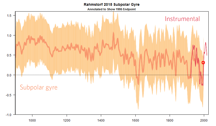
Figure 1. Annotated Rahmstorf et al 2015 Figure 3b. Annotated to show 1995 endpoint. In their running text, Rahmstorf et al say: “The most striking feature of the AMOC index is the extremely low index values reached from 1975 to 1995 … The significance of the 1975-1995 AMOC index reduction was estimated using a Monte Carlo method.”
However, their AMOC reconstruction is defined as the average temperature in 15 gyre gridcells in the Mann et al 2009 reconstruction, which continues to 2006. This raises the obvious questions: why didn’t Rahmstorf show values between 1995 and 2006? Does the withheld portion of the reconstruction between 1995 and 2006 continue to decline?
Once the question is posed, you can guess the answer, which is shown in the figure below, in which the Mann et al 2009 gyre average (blue) is overplotted onto the Rahmstorf et al 2015 figure shown above. Over most of its history, the two series match closely (more or less confirming the provenance). However, instead of the reconstruction, based on Mann et al 2009 gridded data, closing at relatively low 1995 values as shown in the Rahmstorf figure, the reconstruction based on Mann et al 2009 gridded data ends in 2006 at a record high. (By showing this, I absolutely do not imply that this data has any meaning, since I do not agree that a reconstruction of Atlantic ocean currents can be made from contaminated Finnish lake sediments, strip bark bristlecone chronologies etc
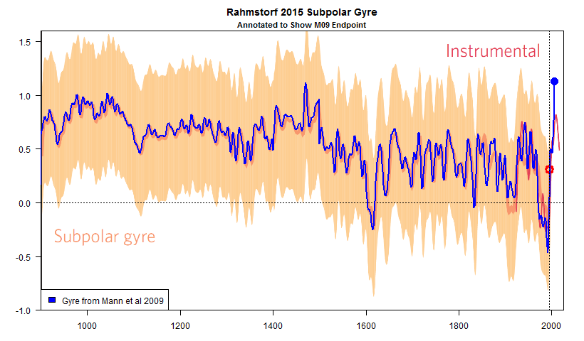
Figure 2. Annotation of Rahmstorf et al 2015 Figure 3b, showing Mann et al 2009 gyre reconstruction (blue), highlighting its closing 2006 value.
The truncation of the subpolar gyre series can be seen in more detail in the zoom below The Rahmstorf series (the muddy “orange” series) ends in 1995, while the calculated gyre series from M09 gridded data goes to 2006. The red series is the GISS instrumental average for the gyre gridcells. The Mann et al 2009 RegEM series is spliced instrumental data in the calibration period – the discrepancy to GISS data appears to arise from differences in instrumental data.
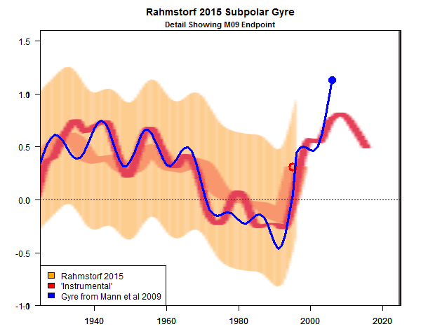
Figure 3. Detail of Rahmstorf et al 2015 Figure 3b, with annotation. The “orange” reconstruction ends ~1995 as shown by the red point. The gyre using Mann et al 2009 gridded data is shown in blue, ending in 2006. The “instrumental” NASA GISS version ends in ~2014-2015. Mann’s RegEM methodology splices instrumental data, but it used a different target instrumental data set.
In Rahmstorf’s Figure 5, he plotted the difference between the gyre series and NH: his pseudo-AMOC index, described as follows:
Figure 5 illustrates corroborating evidence in support of a twentieth-century AMOC weakening. The [light=]blue curve depicts the AMOC index from Fig. 3.
Rahmstorf’s Figure 5 also shows a coral dN15,series: this is a very novel proxy, which had been applied by the coauthors in a 2009 article to assess distance of the coral reef from sewage sources (see here) – the evidence of this article, showing, if nothing else, that the article itself is proximate to a sewage source, if not an actual emitter of sewage. The article cited by Rahmstorf et al (see here) reported results from a Nova Scotia location, saying that d15N values are higher in Labrador current waters and lower in Gult Stream waters. Curiously, we recently discussed alkenone proxies in this region – a proxy which, unlike contaminated Tiljander sediments, might actually shed light on the topic. Needless to say, this was ignored by Rahmstorf in favor of contaminated sediments and stripbark bristlecones.
Once again, I’ve overplotted the difference between the gyre and NH series (the pseudo-AMOC index) using Mann et al 2009 gridded data (blue), once again showing its elevated 2006 closing value. As I understand it, the Rahmstorf 2015 “AMOC index” series was calculated using the gyre series from Mann et al 2009 gridded data – so how it extends to 2014 or 2015 is a mystery for which I did not see any explanation in the article.
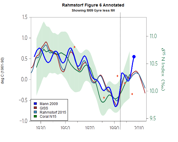
Figure 4. Rahmstorf 2015 Figure 5, showing gyre using Mann et al 2009 gridded data (blue.) Red circle-dot shows closing 1995 value in Figure 3b. Original caption: The blue curve shows our temperature-based AMOC index also shown in Fig. 3b. The dark red curve shows the same index based on NASA GISS temperature data48 (scale on left). The green curve with uncertainty range shows coral proxy data25 (scale on right). The data are decadally smoothed. Orange dots show the analyses of data from hydrographic sections across the Atlantic at 25 N, where a 1 K change in the AMOC index corresponds to a 2.3 Sv change in AMOC transport, as in Fig. 2 based on the model simulation. Other estimates from oceanographic data similarly suggest relatively strong AMOC in the 1950s and 1960s, weak AMOC in the 1970s and 1980s and stronger again in the 1990s (refs 41,51).
Conclusion
Obviously, the most important point about the Rahmstorf reconstruction is its phrenology – i.e. there is no plausible mechanism by which the difference between two linear combinations of unrelated proxies (contamined sediments, bristlecone chronologies, truncated MXD chronologies and hundreds of nondescript tree ring series) can plausibly yield a reconstruction of Atlantic ocean currents as well as separate reconstructions of NH and SH temperature.
But over and above that, there are technical puzzles over the closing values of this data. The Mann et al 2009 gridded data goes to 2006, but the Rahmstorf gyre reconstruction only goes to 1995 in Figure 3. Figure 5 has the opposite problem: the Rahmstorf version goes to 2014/2015, closing on a downtick, whereas the corresponding series calculated from Mann et al 2009 gridded data only goes to 2006 and ends on a uptick.
In my next post, I’ll examine why the Rahmstorf data begins in AD900, though the EIV reconstructions of Mann et al 2009 being considerably earlier.


64 Comments
Being both retired and of limited intelligence I have the luxury of spare time look at your posting to become educated – however, I am really struggling with this post – is it completed?
Familyman-
There seems to be a little leftover/not deleted gobbldygook after the second chart. It could be something that was attached to the chart in the Rahm/Mann noodle paper itself and carried over in a cut and paste and left un-removed. Or perhaps Steve meant to include another figure that isn’t showing up. I lean towards an editing lapse myself.
The main point of this posting is very complete and obvious though….scientists omitting inconvenient data.
Being ironic about the irony there Familyman? Very cutting indeed as if we haven’t already had enough cutting posts 😉
The post was, as you observe, incomplete. I accidentally pressed Publish, instead of Save Draft. The comments on the first two figures were more or less as I intended, but I had other material in my browser and still to be written. The post is now finished.
Gulf Stream watermass change at record levels. It’s catastrophe, Jim, just not as we knew it five days ago.
This latest hockey starts in 1998-2000. How odd. Must be that missing ocean heat content.
“Once the question is posed, you can guess the answer”
Bless their heart…
The divergence since 1995 is attributable to CO2 AGL, Anthropogenic Global Lubrication.
Absorbed Anthropogenic CO2 is decreasing the viscosity of the Gyre, and thus the energy of the Ocean currents despite the contrary appearance. To include bad post 1995 data would obscure the proper trend and makes no sense.
That looks good enough for Climate Science.
A real scientist knows bad data when he sees it and simply deletes it (/sarc just in case)
LOL (or is that Loehle).
Symmetry is a prevalent aspect of all science. It is a persistent property of the universe, occurring everywhere and at all scales.
And, thanks to Steve McI, here we see it again, enriching climate science with “hide the ascent.”
Pat,
I think “Hide the Incline” says in best.
The Team just could not help themselves – snip
Was the pre-1995 plot under a more flattening statistical filter? If so, then a fully flattened graph becomes a hockey stick with no blade, too boring for an important scientific paper.
But it does not matter….
I’m having difficulty finding Mann et al 2009 gyre reconstruction. Does anyone have a link?
M&R 2015 ref. this paper:
Mann, M. E. et al. 2009 Global signatures and dynamical origins of the Little Ice Age
Click to access MannetalScience09.pdf
but I cannot see an SPG reconstruction in there.
Jaime, M&R 2015 constructed the gyre using the temperature proxy reconstructions from Mann, et al., 2009, which itself does not have any gyre reconstructions.
As I understand it, Steve McI’s point is that if M&R, 2015 had used the entire Mann, ea, 2009, data set through 2006, their gyre reconstruction would have terminated as shown in the second figure above, with an ascent.
But they somehow, certainly inadvertently, truncated the Mann, et al., 2009 proxy at 1995, accidentally excluding the unbeknownst-to-them inconvenient 1996-2006 ascending wiggle.
Ah, right. Now I see. Thanks.
Jaime writes:
Quite so. I calculated the SPG series as the average of the gyre gridcells (as shown in Rahmstorf 2015) extracted from the Mann et al 2009 gridded data here
Here is an extraction script, which yields a series from AD500 to 2006.
loc="http://www.meteo.psu.edu/holocene/public_html/supplements/MultiproxySpatial09/longlat" dest="d:/temp/temp.dat" download.file(loc,dest) grid=read.table(dest) dim(grid) #E to W; S to N names(grid)[1:2]=c("long","lat") target$mann=NA for (i in 1:15) target$mann[i]=(1:2592)[target$lat[i]==grid$lat &target$long[i]==grid$long] loc="http://www.meteo.psu.edu/holocene/public_html/supplements/MultiproxySpatial09/allproxyfieldrecon.gz" download.file(loc,"d:/temp/temp.gz",mode="wb") setwd("d:/temp") handle=gzfile("temp.gz" ) test=readLines(handle,n=-1) close(handle) writeLines(test,dest) work=read.table(dest,nrow=2,na.strings="NaN") x=scan(dest)# recon=t(array(x,dim=c(2593,length(x)/2593))) recon=ts(recon[,2:2593],start=recon[1,1]) tsp(recon) #500 2006 index=target$m08 mannrecon= recon[,target$mann] gyre=b= ts(apply(mannrecon,1,mean),start=500) download.file(loc,"d:/temp/temp.gz",mode="wb") dest="d:/temp/temp.dat" setwd("d:/temp") handle=gzfile("allproxyfieldrecon.gz" ) test=readLines(handle,n=-1) close(handle) writeLines(test,dest) work=read.table(dest,nrow=2,na.strings="NaN") x=scan(dest)# recon=t(array(x,dim=c(2593,length(x)/2593))) recon=ts(recon[,2:2593],start=recon[1,1]) tsp(recon) #500 2006 index=target$m08 mannrecon= recon[,index] gyre=b= ts(apply(mannrecon,1,mean),start=500)Thanks Steve. Makes sense now. I guess that M&R would have done the same but neglected to go past 1995. Strange.
My main problem is I just can’t see the SPG being colder during 1975-95 than what is shown in the historic reconstruction during the LIA. Doesn’t make sense to me.
I suspect the problem lies with the lack of temporal resolution of the historic proxy data compared to the instrumental and, even though the proxy data supposedly matches the instrumental very well up to 1995, this seems to be as a result of ‘calibrating’ the proxy data. I quote:
“The surface temperature field is reconstructed by calibrating the proxy network against the spatial information contained within
the instrumental annual mean surface temperature field over a modern period of overlap between proxy and instrumental data (1850 to 1995)using the RegEM CFR procedure additional minor modifications.”
Steve: you say: “My main problem is I just can’t see the SPG being colder during 1975-95 than what is shown in the historic reconstruction during the LIA. Doesn’t make sense to me.” Why on earth would you think that a reconstruction of SPG temperatures using contaminated Finnish sediments and stripbark bristlecones would yield something sensible about the LIA? Why on earth would you put more credence into Rahmstorf’s results than phrenology?
Steve, I think you are unfair to phrenology. What Rahmstorf et al. are indulging in is much more similar to Terry Pratchett’s science of retrophrenology, where you bash people on the head with a mallet until they develop bumps where you want them.
Not Reconstructions, but Procrustean Constructions.
====================
Steve
Are you not anticipating his answer to the 2006 cut off? He’s already said, regarding observations of ocean currents, that recent short term data is irrelevant compared to the older long term picture.
I’m new to this temporally and in knowledge. Been reading all afternoon the criticisms of Mann et al (2008) and Mann et al (2009), and his use of the Tiljander data series. Your criticisms of the continued use, and journal acceptance, of discredited proxy data is right on.
I believe you have already stated that the paleoclimate community needs to join forces in curtailing the misuse of the data. Do you have connections/influence in that community? From my reading it appears that it is largely unpoliticized, and there are many who can be trusted; honestly describing the limitations of their data.
Richard
Steve: there is no interest in the “community” in confronting these problems. People from other climate fields are busy with their own work and presume (incorrectly) that all of this has been investigated over and over and Mann vindicated. Someone like Briffa is undoubtedly aware of the defects, but decided to show solidarity with Mann, because the critics were perceived as subhuman.
That’s how they treated you, in your extreme courtesy. But as you know it doesn’t end with you.
This was inadvertently published before I had finished it. I’ve been out all day and just noticed this.
With all the squiggles it seems more appropriately like anthropomancy.
I’ve finished this post, adding a fair of amount of material that was in my browser earlier in the day as well as some closing text. Apologies for the inadvertent early publish.
Steve
The following conclusion answered a lingering question I couldn’t quite articulate:
“Obviously, the most important point about the Rahmstorf reconstruction is its phrenology”
Thank you
Also, Can you show a comparison of the coral dN15 series used by Rahmstorf and the alkenone series in the region, that you have written about?
Finally, can you recommend a book or article, a primer, on ocean proxies?
Thank you,
Richard
Steve: Im planning to look at the coral data. In the meantime, you might look at
…the evidence of this article, showing, if nothing else, that the article itself is proximate to a sewage source.
You are in fine form, Steve.
“… whereas the corresponding series calculated from Mann et al 2009 gridded data only goes to 2006 and ends on a uptick”.
It looks like Mann’s computer has some sort of malware which causes every time series graph he constructs to end with an uptick.
It’s not malware, it’s by design! If you remember, beyond the contamination aspect of the Tiljander sediment, the non-contaminated part was used upside-down. Mann and his supporters have always said that the direction of a proxy is immaterial and that it will be flipped to create the story.
Ok, they haven’t admitted to creating a story, but they have said orientation doesn’t matter.
It’s un-PC to discriminate on the basis of orientation. 😉
+1. There had to be a reason.
This may be a naive question, but should I conclude that Rahmstorf et al 2015 re using the Mannian device of deciding what they want to portray first and then picking the statistics and data that give them that answer second?
Sorry,”re” should be “are.”
Steve,
“Why on earth would you think that a reconstruction of SPG temperatures using contaminated Finnish sediments and stripbark bristlecones would yield something sensible about the LIA? Why on earth would you put more credence into Rahmstorf’s results than phrenology?”
I don’t, particularly, but I’m looking at the overall pattern over the 1000 years of the reconstruction – warm NH temp/warm SPG during MWP, cooling of both NH and SPG during LIA. So even though the reconstruction from such an exotic collection of various proxies may be highly suspect, I am thinking that it may have captured at least the basic pattern of variability over the period (noting also that NH+3K captures the Medieval warming, subsequent cooling to LIA and then warming into the Modern Warm period). In which case, the huge, seemingly disproportionate cooling of the SPG 1975-95, in combination with its rapid recovery during a period of generally increasing NH temperatures looks suspect.
“Obviously, the most important point about the Rahmstorf reconstruction is its phrenology – i.e. there is no plausible mechanism by which the difference between two linear combinations of unrelated proxies (contamined sediments, bristlecone chronologies, truncated MXD chronologies and hundreds of nondescript tree ring series) can plausibly yield a reconstruction of Atlantic ocean currents as well as separate reconstructions of NH and SH temperature.”
It reminds me of a conversation held at Tamino’s regarding PCA. Each successive orthogonal vector was assigned a different attribute. PC1 – temperature, PC2 – moisture, PC3 — ocean currents apparently, PC4 — likelihood of Mann getting a Nobel prize in physics, etc.. Pure genius! Of course, adding the extra factor of your choosing into the matrix automatically moves all relevant information cleanly to PC1.
Correlation of random noise to random factors is apparently a very entertaining “sciency” job. I wonder if in a thousand years, any of this mathmagic will be used for anything worthwhile.
Excellent point. IOW, meaningless dustbowl empiricism.
Close your mind….
the Force is what gives a Jedi his power. It’s an energy field created by all living things. It surrounds us and penetrates us; it binds the galaxy together.
Nope, it should say— Clear your mind..
This is merely another manifestation of Dirk Gently’s “fundamental interconnectedness of all things.”
We could probably get equally good results with correlating to the lottery, anyone want to try?
Jeff: try Bangladesh Butter Production. It worked for the S&P 500.;-)
http://www.forbes.com/sites/davidleinweber/2012/07/24/stupid-data-miner-tricks-quants-fooling-themselves-the-economic-indicator-in-your-pants/
Jeff, you say..”Each successive orthogonal vector was assigned a different attribute. PC1 – temperature, PC2 – moisture, PC3 — ocean currents apparently, PC4 — likelihood of Mann getting a Nobel prize in physics, etc.. Pure genius!”
======================================================
Are you stating that each disparate proxy used in M.R. is used for disparate aspects of the AMOC flux? Sounds strange. Is the chosen aspect kept consistent throughout the time series?
In other words is the PC2 relationship to moisture, consistent trough the entire 1000 year history? Is the casual relationship established for each proxy to each aspect of the gyre?
Also, this definition of a proxy was used, “hundreds of nondescript tree ring series”. It would appear that with “hundreds of nondescript tree ring series” one could create whatever graphic one wants, depending on the size of your sample to choose from
Sorry for the questions if they appear slow. I am simply not seeing any good description of how each proxy in M.R. was used in determining the speed, salinity, and T of the gyre, nor do I see exactly what portion of the Gyre M.R is applied to OR A comparison to the actual direct measurements of that portion.
David,
My comment was firmly tongue in cheek. There are people who want to believe in these papers so desperately, that they were inventing totally bogus and embarassing relationships as an example of what they thought PCA would do — with tree ring data. I\The ludicrous discussion actually had to do with a Mannian paper where the “proper” hockeystick dropped to PC3 when done correctly. SteveM is the expert on that one.
“one could create whatever graphic one wants, depending on the size of your sample to choose from”
Yup! — https://noconsensus.wordpress.com/2009/06/20/hockey-stick-cps-revisited-part-1/
If the “proxies” really are proxies, then you can extract the true signal through trivial techniques and the results are quite stable even to non-optimal methods.
On the other hand, if the proxies are mostly orthogonal or near-orthogonal, then you are doing something equivalent to the representation of the target series in terms of an orthogonal basis – but not of something usual like Fourier series, but in terms of orthogonal white noise (hundreds of nondescript tree ring series) plus near-orthogonal hockey stick shaped series. It’s easy to get perfect and/or near-perfect representation in a calibration period. When some of the HS series have known persistence, you can get high-RE statistics even if the relationship is spurious.
That I didn’t know. What is Mann’s preferred verification stat, remind me?
Here is a comparison of the Rahmstorf 2015 pseudo-AMOC index to the (smoothed) MBH99 PC1 (which, as archived, was in the orientation shown here “upside down”). Remarkably similar 🙂 The correlation is an astounding 0.67, supporting the surmise that the bristlecones are heavily weighted in the Rahmstorf pseudo-AMOC index:
Here’s an even more amazing comparison between the Rahmstorf pseudo-AMOC index and the MBH PC1. In the figure below, I’ve fitted it stepwise (as done in Mann methods), with steps at 1400,1500, 1600, fewer than actual Mannian methods, but to get an idea. In this representation, the correlation is 0.83!
SteveM, from your comments I take it that Mann(2009) and Mann (2008) use nearly the same proxy data for the reconstructions. If that is the case I know that Mann (2008), besides having all the alterations that you have noted in this thread, uses the nondescript proxy data to which you refer – and I have demonstrated when taken together is much like a series with long term persistence and little or no temperature response – by adding to the large number of proxies which end early so that all proxies end in the year 2006 or there about as I recall. The calculations of the ending additions are not described well in Mann (2008), but nevertheless those additions from whatever source (and some require adding 20 plus years) adds to the tragedy of errors in those reconstructions.
I was thinking that perhaps even an advocate/scientist like Mann might have some shame in using a reconstruction with so much added-in proxy data, but if that were the case he would have had to truncate his current series earlier than 1995. I suspect that if an advocate/scientist was sure in his mind of what the conclusion of a paper should be it becomes easier to justify picking and choosing data depending on the current point you want to make.
Steve: it’s hard to say what he did to extend to 2006. I’m not going to try to guess right now.
I went back and checked the Mann (2009) paper and it is merely applying the Mann (2008) proxy data minus the historical European instrumental records to a network of grids. Thus the gospel according to Mann (2008) is allowed to stand for Mann (2009) and now this paper under discussion here. Interesting how once a climate science paper is published its data and data manipulations can be used without apparent question in subsequent papers.
I was wrong about the end year being 2006 for Mann (2008) it was 1995. All proxies have 1995 as an end year even where data were available only to 1972. See Dataset1 in the SI link below.
http://www.pnas.org/content/suppl/2008/09/02/0805721105.DCSupplemental
I am confused now on how Mann (2009) was extended to 2006. What I see in the paper Mann (2009) is the instrumental data shown in that paper extending that far, but the proxies – like in Mann (2008) only to 1995 as noted in the link below.
http://www.sciencemag.org/content/suppl/2009/11/25/326.5957.1256.DC1
SteveM, I found the data from Mann (2009) that I assume that you have used here and it goes to 2006. I found that data in the SI in a zipped folder that was inside a zipped folder. Nowhere in the main paper do I see a clear statement about the 2006 ending. I would think it has to be using the instrumental data. I see lots of infilling for the reconstruction and instrumental parts.
The 2006 end dates for Mann et al 2009 is, as you’ve acutely observed, not actually mentioned in the article. The 2006 end dates are present in the data plotted in the figures, as in the example below that I checked. We know that M08 and M09 spliced instrumental data and that’s presumably what’s going on.
The Mann et al 2008 reconstruction ends in 2006, though proxies end in 1995.
Oh, what tangled webs are woven
by those to ends, not means, beholden.
“Obviously, the most important point about the Rahmstorf reconstruction is its phrenology – i.e. there is no plausible mechanism by which the difference between two linear combinations of unrelated proxies (contamined sediments, bristlecone chronologies, truncated MXD chronologies and hundreds of nondescript tree ring series) can plausibly yield a reconstruction of Atlantic ocean currents as well as separate reconstructions of NH and SH temperature.”
Please allow me to play Devil’s Advocate.
Say you have 100 proxies. 25 of these are strongly correlated (and indeed, proxies for) air temperature. 25 of these are strongly correlated (and indeed, proxies for) Atlantic ocean currents. 50 of them are just noise or correlated to something else.
If you had an algorithm which assigned weight = 1 (or at least non-zero) to the first group and weight = 0 (or very close to it) to all the rest, you would get a result approximating air temperature.
If you had an algorithm which assigned weight = 1 (or at least non-zero) to the second group and weight = 0 (or very close to it) to all the rest, you would get a result approximating Atlantic ocean currents temperature.
Of course this relies on three very important assumptions: one, that the input data does indeed include proxies for the things you’re looking for, two, that your algorithm is able to distinguish which ones these are and assign weights accordingly and three, that the non-signal parts of the data cancel out sufficiently to yield a good signal-to-noise ratio in the result.
I’m far from convinced about any of those with regards to this paper – especially the second point – but I thought I should point out that it is theoretically possibile.
Steve: The phrenology arises because the “proxies” are unrelated to ocean currents. If one quarter of them were mutually consistent and strongly correlated to ocean currents, then it would make sense to try to tease something from the data. But that’s not what’s happening here.
“Theoretically possible” is not in general a sufficient argument for using a method or set of data (which I know Nicholas knows). Science is supposed to be based not just on plausible methods but on rigorous testing. One’s obligation as a scientist is to examine assumptions and data and if it does not hold up to withdraw a claim. Not to simply ignore serious criticism. When rigor becomes too much trouble, it is no longer science.
Nicholas, I think you, like many others involved in climate science and even those skeptical of the results of reconstructions, are very much missing the point of the biasing done by selecting proxies after the fact by correlating the proxy responses with whatever it is you are attempting to reconstruct. If you have established a criteria a prior for selecting proxies and a criteria which you have developed using some physical basis and you then use all those proxies you might have a fighting chance to allow the unwanted noise to cancel out. That assumes that the noise is random. Also if this process reveals that the proxies do not correlate with the instrumental record you are obligated to go back and revaluate your a prior criteria.
You must from the beginning appreciate the fact that a time series such as that from a proxy that has a reasonably high level of autocorrelation or long term persistence can show a series ending trend corresponding to the trend of the instrumental period and that that correspondence is spurious. If one gets the opportunity to select after the fact and select from a sufficient number of proxies one can select proxies with a spurious correspondence with an instrumental record.
Steve, I think this is where we part ways with The Team. They think that a high correlation is sufficient to “prove” that a series is a proxy and therefore by doing a weighted average of the proxies by correlation they can reconstruct any parameter that might possibly be distantly related. If they were half as smart as they think they are, they’d realise the giant gaping statistical flaws in attempting to do this.
I think you’re right that they can’t possibly hope to extract the data they’re looking for from the proxy series they have but not because it’s mathematically impossible, rather because they’re using incorrect statistical methods and they don’t have enough knowledge of statistics to realise the massive flaws in their approach (or, if you’re cynical, maybe they do but they don’t care).
From what you’ve written (I haven’t read their paper) it seems like they’re claiming the difference in temperature between two regions determines ocean current flow. One of the questions this point raises in my mind is: has this actually been proven or are they just guessing?
Steve: I disagree with you that the problems can be cured with better statistical methods. How can contaminated sediments and stripbark bristlecones and near-white-noise tree ring chronologies tell you anything?
So, Steve, this is rather OT, but were you and Dennis Wingo separated at birth? 🙂
See the video at the lunar orbiter recovery project, here, half-way down the page.
Steve uses the metaphor of phrenology. But technically that should be paleo-phrenology shouldn’t it?
Paleo-phrenology proxies in service of Procrustean reconstructions … and other alliterations in p. So Steve was right to warn us to pay attention to the peas.
Reblogged this on I Didn't Ask To Be a Blog.
A spurious correlation using massively smoothed series – so what else is new in Mannian Statistics? No much. As soon as Mann stops being able to rake in grant money, people will be able to turn around and call it what it is – junk.
Just how, for example, do the Magical Bristlecone Pines of Colorado correlate with the AMOC? Is it the same mechanism that gets these sacred trees the ability to sense the “Global Temperature Field” while being insensitive to local temperature?
8 Trackbacks
[…] Climate Audit finner mer snusk 28.mars Her spør man: Hvorfor viser ikke Rahmstorf i sin figur 3b verdiene mellom 1995 og 2006? Viser de […]
[…] representative of the UK’s jewel in the crown, as he “calls out” some very bad science from Rahmstorf, Mann et al. Notice the deafening sounds of silence from Betts on that thread, […]
[…] Steve McIntyre takes Rahmstorf’s reconstruction methods apart in three very technical posts here , here. and […]
[…] Rahmstorf’s first trick […]
[…] Rahmstorf’s first trick […]
[…] https://climateaudit.org/2015/03/28/rahmstorfs-first-trick/#more-20928 […]
[…] https://climateaudit.org/2015/03/28/rahmstorfs-first-trick/#more-20928 […]
[…] Innen kort tid var RMs arbeid analysert og sterkt kritisert av sentrale fagfolk, deretter fulgte flere kommentarer fra Steve McIntyre da Rahmstorf hadde flere triks. Hele tre til nå. I korthet kan det slås fast […]