Constance Millar, url who wrote an excellent article on the medieval warm period in California, discussed here has written an interesting and timely article (presently in review) on thelate 20th century in the Sierra Nevadas, entitled: Response of high-elevation limber pine (Pinus flexilis) to multi-year droughts and 20th-century warming; Sierra Nevada, California.
For the Hockey Team, time seems have to stood still since 1980 for the collecting of proxies – a phenomenon attributed by Michael Mann to the great expense and heavy equipment needed to core tree rings. I’ve pointed out on many occasions that the warm 1980s, 1990s and 200s offer an ideal opportunity to test out-of-sample validity of the Hockey Team hypothesis that linear indices of tree rings can be used to reconstruct potentially warm medieval temperature. I’ve noted that Hughes collected fresh samples at Sheep Mountain in 2002 and speculated that, if these ring widths had been off the charts, we would have heard about it by now. Because the dog is not barking, it is my hypothesis that ring widths have not been off the charts.
Here is some evidence from nearby high-elevation limber pine that may shed light on the matter. Miller writes: In limber pine, growth was positively correlated with precipitation, minimum temperature, and maximum temperature at low temperatures. This reflects a typical response of high-elevation trees to grow better with more water, warmer nights (minimum temperatures), and relatively warmer days (maximum temperature). Negative correlations of growth with minimum and maximum temperatures at high temperatures, as well as complex interactions of growth with temperature and precipitation, however, suggest that as daytime and summer temperatures increased during the 20th century, limber pine growth declined.
This is not something that would surprise bender or David Stockwell or even me. However, it is inconsistent with the ability of these indices to estimate medieval temperature. Miller goes on to provide an interesting exposition of “significant mortality from 1985 to 1995 during a period of sustained low precipitation and high temperature”. She didn’t mention whether it was “99.98% significant”; perhaps Juckes can assist her with that. She points out that dead trees have lower growth:
Relative to live trees, dead trees over their lifetimes had higher series sensitivity, grew more variably, and had consistently lower growth. While droughts recurred during the 20th century, tree mortality occurred only in the late 1980s.
Her Figure 4C shows the following ring width chronology with a decline in ring widths during the 1980s.

Figure 4C. Growth of secondary rings in limber pine, composite of CLO, DES, and LAU sites; dead trees (solid line), live trees (dotted line).
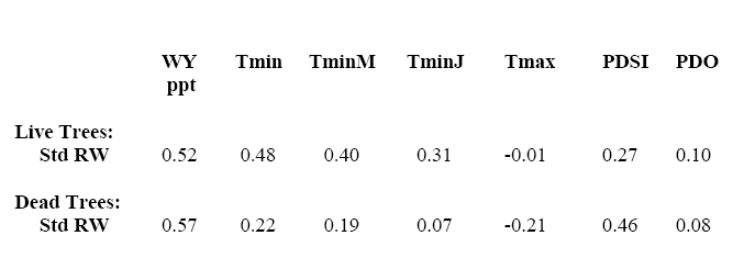
Her Table 3 shows negative correlations with maximum temperatures, positive correlations with minimum temperatures, but even stronger correlations with precipitation.
Table 3. Correlation coefficients of standardized tree-ring widths (Std RW) for live and dead trees at the CLO, DES, and LAU stands with water-year precipitation (WY ppt), minimum annual temperature (Tmin), May minimum temperature (TminM), July minimum temperature (TminJ), annual maximum temperature (Tmax), the Palmer Drought Severity Index (California Zone 5; PDSI), and the Pacific Decadal Oscillator (PDO). Correlations of Tmax and PDO are not signicant; all others have p<0.05.
The NAS Panel failed to analyse the Divergence Problem – the seeming failure of the hypothesis that ring widths have a linear relationship to temperature. In fact, the Divergence Problem has a pretty easy solution – the one stated in two sentences by Millar: at low temperatures, ring widths respond favorably to increased temperature; at high temperatures, ring widths decline. It’s called a non-linear (non-monotonic) relationship. It’s been familiar to biologists and botanists for many years.


24 Comments
Aha, the upside down quadratic. Is it possible to get a temp-moisture interaction term from her data?
Who knows, the moisture term may actually have more impact than the inverse quadratic of temperature. I am picturing a substantial steady upward curve with moisture (waterlogging not really possible in most sites) and a weak upside down quadratic versus temperature, especially for BCPs. You saw me and Mr. Welikerocks’ comments regarding the diurnal and annual normal range in the Whites – namely, immense. Any try that can live there can live in a wide temperature range. And it has to be able to grow at quite low temperatures in order to hit the annual photosynthesis curve right.
try > tree
Ringwidths have positive correlation (at least some) with PDSI? Seems backward unless PDSI is in negative units. Also seems odd in view of the + correlation w/precip.
I’m missing something.
4: Beng, that bugs me, also, unless the index is weird.
4: Beng, that bugs me, also. Maybe the index is “backward.”
Ringwidths have positive correlation (at least some) with PDSI? Seems backward unless PDSI is in negative units.
The Palmer Drought Severity Index does include negative units. -4.0 or less corresponds to “extreme drought,” the range [-0.49, 0.49] corresponds to “near normal,” and 4.0 or more corresponds to “extremely wet.” Details here.
I read most of Millar’s article on the MWP, and I don’t see how anyone could argue that there was a very warm MWP in California. Another great example of using treeline (as well as species diversity) to elucidate climate in the past. Hope some of the Team members take time to read it.
Did you mean I don’t see how anyone could argue that there wasn’t a very warm MWP in California?
Loki. Correct, gotta slow down and read first, then post. Thanks!
There are just so many interesting papers referenced at this site. For example the Millar paper contains, in its abstract, this:
It is no surprise that precipitation is as important or more so in tree growth in many cases, however, it is more complex than even that simple analysis. Parker and others have shown that precipitation in the preceding Fall (September and October) are the best indicator of growth in the subsequent season. Similarly snow cover and amount are also very important factors especially at high altitude and latitude. Finally there is the forgotten moisture that I have written about for farmers and that is condensation. In the late summer and fall moisture from condensation can be very siginificant (inches in a matter of weeks) yet it is never included in the moisture calculatons. Much more uniform and often wider in distribution than rainfall and usually available at night when there is less heat stress it suits the shedding nature of tree structures. That is, condensation accumulates on all leaves or needles and is then funneled to the outside of the tree where it falls on the root structure designed around the periphery as opposed to the tap root that mostly just anchors the tree.
To which anyone who has ever camped among coastal redwoods will readily attest. It “rains” all night long in those forests and well into the morning, too.
This is extremely fascinating. Along the same lines as this study, I was pulling some of the Alpine treering studies (in light of the recent announcement by the Austrian researchers on warming in the Alps), and came across this study by Buntgen et al (2005). http://www.springerlink.com/content/7450113086l86036/
What hit me was the last part of the abstract had this little gem:
Does that really say what I think it says?
Noticed my name in the post I wanted to add my view of plant responses (limitations) these days, though having been reduced to little more than a drive by shooter on this blog, appologize in advance for lack of interactivity.
It seems like we approach the view of plant responses with a temperature/precipitation blinker on, which is fine in so far as they are correlated with these factors and would be good to use a quadratic or ‘humped’ response in models (just a little step up from assumptions of linear response). This view is also consistent with laboratory responses but the situation in natural environments is different.
Tim Ball #12 said:
My experience is that that monthly climate data is in general more predictive that annual data and overall, and the particular variable varies from species to species. The view that each species responds most strongly to a different variables seems to me an inevitable consequence of entropy constraints. I.e. if all species started out respondig to the same variable, over time they would relax into a lower energy state where each was responding differently. This is a kind of intuitive explanation for uniqueness in nature. Given the way measurements are artificial, the variable we choose as human observers is not necessarily the real thing the plants are (limited by) responding to.
So the bottom lines are:
1. There is no apriori reason to think that each species responds best to the same variable.
2. There is no reason to think the more correlated variables stay constant over time.
Still you do the best you can with what you have, and it should be possible to do something, but not without expanded error bars.
#14
Did you read the whole paper? They show their spruce RCS chronology together with Mann99 and Esper02. Not very hockeyish, theirs.
#16
That’s the point I was hoping to make. I’m not a dendro expert though. My expertise is signal processing. Was hoping to get some of those more familiar with dendroclimatology to comment on whether this should be considered another paper which diverges significantly from the accepted hockey-dendro reconstructions.
I never thought my Freshman Alpine Ecology paper would be of significance 34 years later. I sampled Picea abies rings in the Swiss Alps and plotted them against altitude. I found the peak growth rate to be at an elevation of 1450 meters. Above that, the growing season was short, below that, they were competing with deciduous tree. I can’t imagine a worse proxy.
Re: positive correlations with PDSI:
From p. 14:
Re #1
jae: PDSI is, basically, a P*T interaction term. There are other evapotranspiration-based indices that might work better, however.
bender: I haven’t used statistics much in years, and I’ve forgotten a lot. But why can’t you do an AOV, using the model Growth = T + P + TP + e, and determine whether TP explains most of the variation? Maybe info on P is not available?
Mechanically speaking, you could. Of course time-series are not well-suited to AOV/regression approaches. But that wouldn’t stop the team if the output were to favor their hypothesis, would it?
Information on P must be available if they were able to calculate PDSI.
Oh, yeah, I keep forgetting about the time series issues. I’ve been doing some reading, though and am now appreciating some of the intricacies, like autocorrelation.
RE 14:
Does that really say what I think it says?
It depends. What do you think it says?
Best,
D