Tamino’s guest post at RC deals with global mean temperature and AR(1) processes. AR(1) is actually mentioned very often in climate science literature, see for example its use in the Mann corpus (refs (1,2,3,4). Almost as often something goes wrong (5,6,7). But this time we have something very special, as Tamino agrees at realclimate that AR(1) is an incorrect model:
The conclusion is inescapable, that global temperature cannot be adequately modeled as a linear trend plus AR(1) process.
This conclusion would be no surprise to Cohn and Lins. But if their view is that global temperature cannot be adequately modeled as a linear trend plus AR1 noise, what are we to make of IPCC AR4, where the caption to Table 3.2 says
Annual averages, with estimates of uncertainties for CRU and HadSST2, were used to estimate. Trends with 5 to 95% confidence intervals and levels of significance (bold: less than 1%; italic, 1 – 5 %) were estimated by Restricted Maximum Likelihood (REML; see Appendix 3.A), which allows for serial correlation (first order autoregression AR1) in the residuals of the data about the linear trend.
This was mentioned here earlier (9). Thus, according to Tamino the time series in question is too complex to be modeled as AR(1)+ linear trend, but IPCC can use that model when computing confidence intervals for the trend!
But there is something else here, how did Tamino reach that conclusion? It was based on this figure:
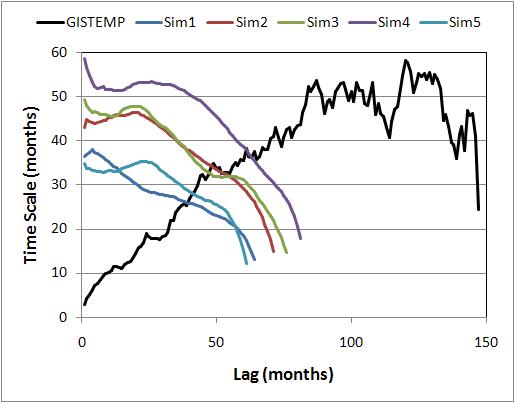
It would be interesting to try to obtain a similar figure, here’s what I managed to do :
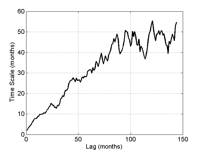
First, download (10) and arrange data to one 1530X1 vector. Divide by 100 to get changes in degrees C. Then some Matlab commands,
n1=detrend(data); % Remove a linear trend, center
[Xn,Rn]=corrmtx(n1,12*12); % Autocorrelation matrix
% note that signal processing guys sometimes
% use odd definition for correlation vs. covariance
% (not center vs. center)
cRn=Rn(:,1)/Rn(1,1); % divide by std
fi=find(cRn<0); % find first negative
if isempty(fi)
fi=12*12+2;
end
thn=-(1:fi(1)-2)’./(log(cRn(2:fi(1)-1,1))); % -dt / ln
plot((1:fi(1)-2)’,thn,’k’)
Black line is quite close:
Next step is trickier, how to make those AR(1) simulations? For a monthly data, tau=5 years= 60 months. Should we use one-lag autocorrelation p=0.985 then? 5 realizations in red color:
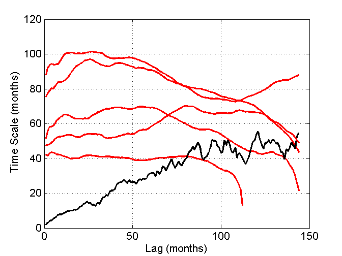
Not a good idea. How about AR(1) with p=0.985 + some white noise, again 5 realizations in red color:
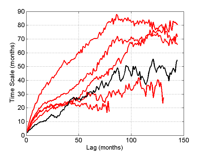
Much better. No wait, I was trying to replicate Tamino’s simulations, not the GISS data result. Any suggestions?
UPDATE(SM): Lubo has an interesting post on this , also linking to a paper coauthored by Grant Foster and realclimate
Click to access comment_on_schwartz.pdf
References
1 http://www.realclimate.org/index.php/archives/2006/05/how-red-are-my-proxies/
2 Mann, M.E., Lees. J., Robust Estimation of Background Noise and
Signal Detection in Climatic Time Series , Climatic Change, 33,
409-445, 1996.
3 Mann, M.E., Rutherford, S., Wahl, E., Ammann, C., Robustness of
Proxy-Based Climate Field Reconstruction Methods, J. Geophys. Res.,
112
4 Trenberth, K.E., P.D. Jones, P. Ambenje, R. Bojariu, D.
Easterling, A. Klein Tank, D. Parker, F. Rahimzadeh, J.A. Renwick,
M. Rusticucci, B. Soden and P. Zhai, 2007: Observations: Surface and
Atmospheric Climate Change. In: Climate Change 2007: The Physical
Science Basis. Contribution of Working Group I to the Fourth
Assessment Report of the Intergovernmental Panel on Climate Change
[Solomon, S., D. Qin, M. Manning, Z. Chen, M. Marquis, K.B. Averyt,
M. Tignor and H.L. Miller (eds.)]. Cambridge University Press,
Cambridge, United Kingdom and New York, NY, USA.
5 http://www.climateaudit.org/?p=682
6 http://www.climateaudit.org/?p=370
7 http://www.climateaudit.org/?p=1810
8 http://en.wikipedia.org/wiki/Ornstein-Uhlenbeck_process


137 Comments
For the benefit of the EEs here, AR(1) is roughly the same thing as an IIR.
Read this.
I find it extremely disturbing that neither Schwartz, Tamino, Foster, Annan, gavin nor mike seems to have ever heard of Partial Autocorrelation function, which is recommended as the first check for autoregressive models in any modern introductory text to time series. I guess Box-Jenkins (more e.g. here) is something completely unheard of to these people. Would it be time finally to actually contact people who know something about time series analysis?!?
If any of the above mentioned people happens to read this, PLEASE read e.g. Shumway&Stoffer’s book. It contains plenty of worked out examples (with R code!) and example data series including Jones’ (1994?) global temperature series and plenty other climatology related data. It also teaches you how to handle seasonal data, so you won’t be confusing between autoregressive models with yearly data with the autoregressive models with monthly data…
Lubos Motl did a greatpost on it yesterday:
http://motls.blogspot.com/2007/09/stephen-schwartz-vs-scientific.html
Some R code. Not every realisation matches Tamino’s plot, but a good proportion do.
GISTEMP.src=”http://data.giss.nasa.gov/gistemp/tabledata/GLB.Ts.txt”
GISTEMP=read.fwf(GISTEMP.src,c(5,rep(5,12),7,4,7,5,5,5,6),header=F, skip=7, as.is=T, nrow=140)
colnames(GISTEMP)=GISTEMP[1,]
GISTEMP=apply(GISTEMP,2,as.numeric)
GISTEMP=GISTEMP[!is.na(GISTEMP[,1]),1:13]
GISTEMP=as.vector(t(GISTEMP[,-1]))/100
gis.res=resid(lm(GISTEMP~I(1:length(GISTEMP))))
lag.cor=acf(gis.res,lag.max=180)
Tau=-(1:180)/log(lag.cor$acf[-1])
plot(1:180,Tau, col=1, lwd=2, ylim=c(0,100))
for(i in 1:5){
sim=arima.sim(list(ar=.984),n=125*12)
sim.res=resid(lm(sim~I(1:(125*12))))
lag.cor.sim=acf(sim.res,lag.max=180, plot=F)$acf[-1]
lag.cor.sim[(1:length(lag.cor.sim))>min(which(lag.cor.sim
> fixed
#import data
GISTEMP.src=”http://data.giss.nasa.gov/gistemp/tabledata/GLB.Ts.txt”
GISTEMP=read.fwf(GISTEMP.src,c(5,rep(5,12),7,4,7,5,5,5,6),header=F, skip=7, as.is=T, nrow=140)
colnames(GISTEMP)=GISTEMP[1,]
GISTEMP=apply(GISTEMP,2,as.numeric)
GISTEMP=GISTEMP[!is.na(GISTEMP[,1]),1:13]
GISTEMP=as.vector(t(GISTEMP[,-1]))/100
gis.res=resid(lm(GISTEMP~I(1:length(GISTEMP))))#detrend
lag.cor=acf(gis.res,lag.max=180)
Tau=-(1:180)/log(lag.cor$acf[-1])
plot(1:180,Tau, col=1, lwd=2, ylim=c(0,100))
for(i in 1:5){
sim=arima.sim(list(ar=.984),n=125*12)
sim.res=resid(lm(sim~I(1:(125*12))))#detrend
lag.cor.sim=acf(sim.res,lag.max=180, plot=F)$acf[-1]
lag.cor.sim[(1:length(lag.cor.sim))>min(which(lag.cor.sim<0))]=NA
Tau.sim=-(1:180)/log(lag.cor.sim)
lines(1:180,Tau.sim, col=2)
}
#17, Hi Richard
Could you post a plot?
I couldn’t get it to run out of the box, but I’m an R newbie so don’t worry about that.
Thanks for the code! It will give me something to learn from.
This Schwartz paper is getting a lot of attention. The anti-AGW sites are busily promoting it. The AGW sites are busily refuting it.
Rightly or wrongly, most people put this site squarely on the anti-AGW (denier) side. In my opinion, it is different than many anti-AGW sites because SteveMc is capable of understanding and auditing the science.
With that in mind, I think it would be very interesting for SteveMc to audit the Schwartz paper.
RE 29.
John V.. We’ve suggested that, but SteveMc is looking for something a bit more
foundational ( In UHI studies for example, everybody cites, peterson and Parker)
Is that fair SteveMC? basically, there is no point in auditing a paper like schwartz
which the AGW crowd has already trash binned.
ONE ethos here is verifying what has been accepted.
29:
I proposed this some time ago, and was told that it is not sufficiently “authoritative>” I think it is a great paper. Maybe not perfect, but worthy of discussion. But this site is not devoted to auditing technical stuff, just statistical stuff.
Re suggestions: Ask him on his blog.
Re30, it seems very odd that a variable star specialist would ignore any solar variability in his review of driving and feedback mechanisms.
http://tamino.wordpress.com/2007/09/05/graphic-evidence/
But the comparisons seem valid otherwise.
I don’t recall saying that.
IT looks like an interesting paper. HOwever, I’ve only got a certain amount of time, I can’t do everything in the word. I also try to do things that other people aren’t doing and it looks like other people are writing on Schwartz. I’d like to get to it some time.
Has anyone had any luck with the script posted by richardT in #17?
Apologies if my anonymity disturbs you, remember that I’m not the only one, see e.g. http://en.wikipedia.org/wiki/William_Sealy_Gosset
Hmm, I haven’t submitted anything to a climate science journal (yet.. 🙂 ), so maybe I’ll use this excuse:
http://en.wikipedia.org/wiki/Peer_review :
Back to business, we have a figure to replicate. richardT , did I understand correctly, you detrend the simulated series as well?
UC, many thanks for posting up the details of this.
The irony that realclimate suddenly don’t like AR(1) plus trend is gobsmacking. Tamino suddenly wants to do Monte Carlo tests, shame s/he wasn’t so proactive when it came to Ritson’s “novel” estimation process, or any of the other issues that have been raised here. It also shows the difference between people who are well versed in statistics (UC, Jean S) and those who dabble (Tamino, Mann etc).
It is also a shame people are upset by Tamino’s anonymity, which is not relevant to the science, and have sidetracked a very interesting thread. This could be a turning point for RealClimate: the discovery of model misspecification 😉
Bourbaki.
I’m relatively untutored in statistics. Could some one explain the meaning of graphs in simple language?
#51/#52: Theoretically, a straight line. BTW, IMO it’s not enough to be “tutored in statistics” to understand those figures. The idea behind Schwartz \tau estimation and those graphs is that if you have AR(1) process the autocorrelation decays exponentially with respect to the lag, i.e.
 . You can solve that equation for
  and those plots are h vs.
  using estimated
  (sample autocorrelation).
The weakness in Schwartz’s estimation comes from the fact that he’s using that equation to estimate in the context of AR(1) process. This is what those rebuttals are attacking. They try to show that
1) the process really isn’t AR(1)
2) even if it were, Schwartz’s estimation gives a biased (in statistical sense) answer
What I find disturbing (see #10) is that Schwartz didn’t provide PACF-plots (for the defense) and neither others for offense (for the case 1) ). It should be the first thing to do when deciding if a process is AR(1) or not. However, there is a thing which seems to have been missed by all of them: the process does not need to be AR(1) for the exponential decay of the autocorrelation (which, if I have understood correctly, is the main thing behind Schwartz’s idea of estimating the “relaxation time constant”). Any stable ARMA process with real roots is enough. So this implies, that if one accepts the premises given in the beginning of Schwartz’s section 4, the method is not necessarily invalidated even if the criticism point 1) would be true. Also notice that such an ARMA process could be generated, for instance, by a linear combination of individual AR(1) processes. This should be acceptable even to Foster et al, see the first two paragraphs in their section 2 (although the speculation in the second paragraph is nonsense).
However, before anybody draws any conclusions that I’m saying that Schwartz’s method is reasonably correct, there is another thing which has been overlooked by all the parties: in order for the Schwartz’s idea to work, it is necessary that the underlying (detrended) process (wheather it is AR(1) or general ARMA) is stationary. However, there is some evidence (see Shumway & Stoffer) that this is not the case.
Jean S. #53,
OK that is kind of what I thought.
If we look at 60% (1 – 1/e) of the maximum we get a number of around 60 months. Is that the correct way at looking at this?
BTW I got your time constant stuff. Every day electronics in a single lag system.
It would be interesting to see climate modeled as a series of RCL networks with voltage controlled current sources and current controlled voltage sources (amplifiers). A lot of the disputes seem to be similar to the capacitor soakage problem in electronics. Where you have a dominant lag (for short term variations) and decoupled lags on longer term scales.
I think an electronic model would eliminate a lot of hand waving.
SteveM, thank you for drawing attention to this new and welcome development at RC. It seems that RC is finally rejecting the idiotic position previously promoted by Rasmus, and endorsed by Schmidt and Mann, for iid or AR(1) noise in the temperature signal. Excellent!
But where does this lead? Can we assume that RC now endorses Koutsoyiannis’s finding that long memory is ubiquitous in hydroclimatological time series? Following this line of reasoning, would it be safe to say that RC now recognizes that observed climate trends are of indeterminate statistical significance?
😉
Now, not doing the math, does not empirical evidence support the 1.1 +/- .5 degree C sensitivity? The CO2 level has gone up from 280 to 390 which is a 39 percent increase. The temperature in the same period has gone up ~0.6 degree C. Now if you take that out to doubling, there is only going to be ~ 1.5 degree C increase based on the current trend. If the sensitivity is higher than the 1.5 degree C it appears to be now, where is all the warming hiding? Why has there been no warming since 1998? CO2 has gone up.
This is based on the alarmist own numbers (which I do not have that much faith in) but still only shows 1.5 degree C for doubling of CO2. This is the very low end of the IPCC and well below the 2-7.5 used in most models.
re 57:
It’s those cooling aerosols (that don’t cool China BTW).
I’ve either deleted or moved a number of posts dealing with anonymity – which affects the numbreing.
richardT,
(http://www.climateaudit.org/?p=2047#comment-139800 ? )
Detrending makes autocorrelation estimates smaller, and the comparison was supposed to be detrended GMT data vs. AR(1). Try to obtain a 5 sample set, where all series end before Lag=100, without detrending. Options are
1) Tamino’s simulations are detrended AR(1)s p=0.985 , and the sample is not very representative
2) Tamino’s simulations are AR(1)s p=0.985, and the sample is far from representative
3) Tamino’s simulations are something else
Maybe we should ask Tamino to free the code.. Nah,
richardT:
That’s true, but you can add white noise after generating AR(1) which results ARMA(1,1) process – then short lag results will go down. See Jean S’ post, that shouldn’t change Schwartz’s conclusions ( not that I agree with Schwartz, all those people should take some math lessons before writing math-related journal articles)
RE19 “I think an electronic model would eliminate a lot of hand waving.”
I’ve been thinking about exactly the same thing to model a temperature observation station, since diurnal temperature variations roughly approximate a sine wave.
RE19 I’ve been thinking lately that the whole data measurement, rounding, gathering process, USHCN adjusments, and output essentially amounts to an electronic low pass filter network.
Given that, as you say it might be useful to explore how biases and noise signals propogate through such an electroinc model. Parallels can be drawn to voltage, current, resistance, and capacitance to the real world environment of temperature measurement.
re 25.
Yup! Same thing for Tmax and Tmin, but you have to look at daily’s to see it
#27. The CRN data has all the time detail that one could want. The dirunal cycle seems to be a somewhat damped sine wave as (Tmax+Tmin)/2 is higher than the average at the CRN stations i.e. the low seems to be damped from a sine wave.
Anthony (#12),
Try Figure 16.
Vernon (#21),
That is an interesting question. Few people seem to be discussing what are the fundamental differences between what Schwartz did and what mainstream estimates do. It’s not like Schwartz is the first to consider AR(1) processes or energy balance models in estimating climate sensitivity. Schwartz himself should have spent more time explaining how his methods differ from others, and why he gets a result so far from the mainstream.
One major difference, and where IMHO Schwartz’s fundamental error lies, is in the treatment of the oceans. Hansen et al. (1985) noted that the climate response time depends heavily on the rate at which the deep ocean takes up heat. High climate sensitivities can look very similar to low sensitivities if the rate of heat uptake by the ocean is high, due to the amount of unrealized warming over times smaller than the equilibration time of the climate system. Unfortunately, that rate is not well constrained.
Schwartz, unlike most modern papers on climate sensitivity, does not truly couple his energy balance model to a deep ocean: he tries to just lump the atmosphere and the ocean together into a homogeneous system. I suspect that if he did couple to a deep ocean, even with a simple two-layer model like Schneider and Thompson (1981), he would get very different results. (Probably you need a full upwelling/diffusion model such as Raper et al. (2001).) You really need to jointly estimate climate sensitivity and vertical diffusivity of the ocean, and the uncertainty in the latter makes a big difference to estimates of the former. (As does uncertainty in the radiative forcing; Schwartz’s analysis neglects independent estimates of the forcing time series, which is probably another reason his results disagree with mainstream papers.)
This is one of Annan’s main points on his blog, which is that you can’t really ignore the existence of multiple time scales in the climate system. A straight time series analysis over a ~100 year period is going to be dominated by the large, fast atmospheric responses. We only see the transient response. But climate sensitivity is about the long term equilibrium response, and there you can’t ignore the slower processes like oceanic heat uptake, which are harder to estimate from the time series alone unless you’re very careful, but which greatly influence the final estimate. Treating the system as if it has just one time scale means that you’re not really getting either the atmospheric or the ocean response times right.
Wigley et al.’s 2005 JGR comment to Douglass and Knox is another example of the issue, showing how hard it is to estimate climate sensitivity without a careful treatment of timescales, and the problem of using fast-response data (like volcanoes) to constrain the asymptotic equilibrium behavior of the system.
See Tomassini et al. (2007) in J. Climate for a nice modern treatment of this problem, which attempts to use ocean heat uptake data to constrain the vertical diffusivity. They are not the first to do so, but I think it’s one of the best published analyses to date from the standpoint of physical modeling and parameter estimation methodology. But they unfortunately ignore autocorrelation of the residuals entirely! There are people who have done good time series analysis, and people who have done good climate physics, and they need to talk more. Schwartz’s paper, unfortunately, appears to have done neither.
26, see comment 1. Any linear dynamic system can be viewed as a filter in the frequency domain without loss of generality. The only assumption is linearity, which is always a reasonable assumption for small perturbations.
Lubo has an interesting post on this , also linking to a paper coauthored by Grant Foster and realclimate
Click to access comment_on_schwartz.pdf
30 addendum – of course, if you do this, the frequencies are complex numbers. You have to keep track of phase relationships.
31, With Annan, Schmidt and Mann. It’s always the same small cast of characters that end up defending the overwhelming consensus, isn’t it?
One of the big advantages of the electronic model is that you can draw circuit diagrams. A picture is worth… a lot.
Re#31, interesting to see “Zeke’s” comment http://julesandjames.blogspot.com/2007/09/comment-on-schwartz.html#362301877944802755
Seems to be an admission that peer review and publication is about names, not substance.
Another advantage is that it shows the elements of the model as isolated components. Each of which can be given a value.
Then you can start to do science by working on the values of isolated elements instead of the hoge poge we get now with everything scrambled.
We are already seeing that with Schwartz. Short time constant? Long time constant? A mix?
I’m going to do a stupid simple diagram and post it to get the ball rolling.
>> Im going to do a stupid simple diagram and post it to get the ball rolling
You could start with the one in the Ozawa paper.
#29. You’re not commenting on one of UC’s main point: what’s sauce for the goose is sauce for the gander; if this is what they think, then they cannot argue that IPCC’s goofy and botched use of Durbin-Watson could be used to reject the review comments against their attempts to attribute statistical significance to trends.
“you cant really ignore the existence of multiple time scales in the climate system”
I believe that Schwartz explicitly pointed out that it was his intent to ignore the vertical ocean water mixing and look at things from a shorter term, higher frequency signal basis. In the longer term it would seem like the total heat of the Earth is being reduced. The rate of ocean heating due to underwater vulcanism doesn’t seem to be well understood as far as I know.
The relatively large variation in the measurement results of the annual quantity of heat in the atmosphere and upper layer of the oceans either indicates a very imprecise measurement system or a lack of understanding of the daily/weekly/monthly/annual forcing functions and the system response over a similar time span. There seem to be two ends to lack of understanding of “climate” processes in the time domain. Schwartz was attempting to estimate the magnitude of a certain part of the time response of the very complex system.
From recent discussions, the consensus seems to be that climate prediction is only deemed to be potentially valid starting at about ten years out. I’d guess that there is a great interest in getting to accurate predictions on the order of a year. Not being able to do that would indicate a lack of understanding of all the important variables in the annual time frame (along with predictive capabilities regarding much of the sources of actual system input forcings).
The “missing” atmospheric warming is due primarily to the thermal inertia of the ocean. I don’t know exactly when this was first proposed, but the Charney Report described it 28 years ago.
29
Correct.
Wrong. The exercise is to deduce climate sensitivity, which in itself is a consequence of very fast processes, from it’s lagged response, which is a much slower phenomenon. The only thing that matters is that the lag in the oceans is much greater than the greenhouse warming itself.
I think you mean the spectral components within a given frequency bin are complex, not the frequencies themselves, which are necessarily real numbers.
Mark
Larry (#41),
“The exercise is to deduce climate sensitivity, which in itself is a consequence of very fast processes, from its lagged response, which is a much slower phenomenon.”
I don’t think you are disagreeing with me. The point is not whether the value of climate sensitivity is dominated by fast processes (e.g. water vapor and cloud feedbacks), but that any long term equilibrium behavior is going to be hard to diagnose from the response time series without taking into account longer term climate processes such as the oceans.
Gunnar,
Do you have a link to the Ozawa paper? I couldn’t find it on CA.
PI says:
No it doesn’t. It’s a pretty well established model in ocean transport that there’s a “mixed layer” which is turbulent, and thus well-mixed, and the remaining water beneath it is quiescent, and transport is orders of magnitude lower. That means that for practical purposes, the part of the ocean that interacts with the atmosphere is only about 100m deep. If you try to incorporate the rest of the ocean into models using short-time response, you’ll get a wrong answer.
http://www.hpl.umces.edu/ocean/sml_main.htm
No, not true at all. The “frequency” is a real number, generally either f or omega. The spectral component is a complex number, though not the frequency itself. The complex representation of a sinusoid is a*exp(j*2*pi*f*t) = a*exp(j*omega*t), and the frequency itself is f (in Hz) or omega (rad/s), which is real by definition (f=c/lambda, both of which are real numbers).
Mark
46, it’s safe to assume that a 5 year e-folding time is >> than any atmospheric processes.
Larry,
#48: You don’t treat the mixed layer and the deep ocean with a short time response, or for that matter with the same response.
#50: What’s your point?
Oh dear!!! I came accross this paper:
John Haslett: On the Sample Variogram and the Sample Autocovariance for Non-Stationary Time Series, The Statistician, Vol. 46, No. 4., pp. 475-485, 1997. doi:10.1111/1467-9884.00101
Well, what are the results? He considered various models for fitting the NH tempereture series (1854-1994, Jones’ version I think):
Well, that’s the Schwartz’s model with the exception that Haslett uses ARMA(1,1)-model (AR(1)+white noise)! If I’m not completely mistaken, the REML-fitted values (AR coefficient=0.718) means a decay time (Mean lifetime; Schwarz’s ) of -1/log(0.718)=3.0185 years!
54, For the purposes of 5 year dynamics, the mixed layer is homogeneous, and the rest of the ocean doesn’t exist. There might as well be a blanket of insulation between the two layers. That’s exactly why the long-term dynamics don’t matter.
Larry,
The long term dynamics do matter to the long term equilibrium response.
Jean S,
What is your opinion of Wigley et al., GRL 32, L20709 in this context?
I’ve moved a number of posts to Unthreaded.
“This paper consists of an exposition of the single-compartment energy balance model that is used for the present empirical analysis, empirical determination of the effective planetary heat capacity that is coupled to climate change on the decadal time scale from trends of GMST and ocean heat content, empirical determination of the climate system time constant from analysis of autocorrelation of the GMST time series, and the use of these quantities to provide an empirical estimate of climate sensitivity.”
Certainly sounds like no second compartment containing longer than decadal heat capacity considerations to me (along with exclusion of all sorts of other personal favorite mechanismz).
That’s what I did in the last figure. I should apply funding from some pro-AGW program 🙂
Some questions I have in my mind..
Haslett:
So no drift is also a possibility? What kind of process should we assume for measurement errors?
Regarding Emanuel’s
If greenhouse gases cause that drift, why do we need aerosols ? Are they trying to simulate AR(1) component as well?
MannLees96 robust procedure (*) yields tau = 1 year for global average. Is he talking about same tau as we are here?
(*) AR(1) fit to median smoothed spectrum
Oh dear again!!!! UC:
Yes, it is indeed the same (see eq (3))! In fact, Mann’s model in section 6 is exactly the same as Schwartz’s
(linear trend+AR(1))! Foster et al:
Mann & Lees (1996):
What a clown this Mann is.
Additionally, we have an estimate for $latex \tau[\tex] (=2) in
Allen& Smith: Investigating the origins and significance of low-frequency modes of climate variability, GEOPHYSICAL RESEARCH LETTERS, VOL. 21, NO. 10, PAGES 883886, 1994.
http://www.agu.org/pubs/crossref/1994/94GL00978.shtml
So we have the following ranking:
Mann&Lees: 1
Allen&Smith: 2
Haslett: 3
Schwartz: 5 \pm 1
And now the RC-folks are saying that Schwartz’s estimate in an underestime. This is a complete farce.
Jean S, I think soon they will tell us that “Idiots, it is different tau, pl. study some climate science’” .
Meanwhile, let’s try to figure out why those values are small at small lags:
Assume that we have AR(1) process x, p=0.9835. Without loss of generality, we can assume that it’s (auto-cross) covariance matrix A diagonal elements are ones. Due to measurement noise or whatever, another process is added to this process, a unity variance white noise process. It’s covariance matrix is I. Assuming these processes are independent, the resulting process y has a covariance matrix
B=A+I
and in this case it is just a correlation matrix of x, but diagonal elements are twos instead of ones. To obtain correlation matrix, we just divide all elements by two:
D=B/2
Autocorrelation function of x is with lags 0,1,2 and so on. For this new process they are (take first column of D)
  and so on. The relation between tau and p is p= exp(-1/ tau ), and thus theoretically
which is the basis for Scwartz’ plots. However, if the process is AR(1)+ white noise, we’ll get for non-zero lags (n)
As n get’s larger, this value approaches tau. Here’s a simulation, realizations of y as defined above, and this theoretical function:
( http://signals.auditblogs.com/files/2007/09/simul1.png )
hmm,
UC, correct me if I got it wrong: you are saying that Schwartz’s figure 7 is actually very consistent with Haslett’s model!
BTW, Mann & Lees (1996):
Jean S.,
Are all these people really talking about the same problem? I think you need to be more careful and read the articles thorougly. So far I know it is generally believed that the the heat uptake by the ocean has a very long time scale. Few will dispute that.
#61 gb, for the purposes of this discussion, no one’s arguing the scale of the uptake. The issues are entirely mathematical given any specification that climate scientists care to choose. The problem is the total inconsistency and incoherence of the practitioners.
Well, I’ve done that. Did I miss something? I don’t know what difference it makes if they intend to talk about the same thing, if they have the same data (global/hemispheric temperature series), the same model (trend+AR(1), or in the case of Haslett, trend+AR(1)+white noise) and they estimate the same parameter (mean lifetime of the exponentially decaying autocorrelation function)?
If this parameter is not actually meaningful in Schwartz’s calculations, then that’s the refutation the paper and that should be written to the journal. I’m not discussing that.
I did some notes about 2 years ago on ARMA(1,1) models. They fit most temperature series better than AR1 series and yield higher AR1 coefficients (often over .9) and negative MA1 coefficients. Perron has reported some serious difficulties in statistical testing in econometrics for these “nearly integrated nearly white” series.
UC:
We didn’t have to wait too long…
UC says:
September 21st, 2007 at 7:32 am
Thanks for that.
The blue line clarifies a lot for me!!
Concerning the deep mixing of the oceans, I have one point and one question.
The main point is that most of the deep ocean mixing is via cold, circumpolar downwelling and more tropical upwelling. Since the water which sinks is mostly near zero degrees C, it’s not going to warm the deep ocean, though it will, if the upper waters contain more CO2 than the deep waters, sequester some CO2. But so far, I think, the deep waters still have more CO2 in them than the upper waters so that the net result is to dilute deep waters slightly in CO2.
The question I have is if we imagine that all the surface water which mixes by diffusion with either the deep or mid ocean waters directly rather than by sinking near the poles could be calculated, how much volume would it be compared to the amount of water which sinks at the poles? I realize it a bit of a problem since the temperature of the mixed layer varies over the earth’s surface. So I’m not sure how this could be determined except perhaps via isotope studies (from Nuclear explosions for instance).
Anybody have a reference which I could look at?
For Jean S:
Haslett’s paper is on NH only, correct?
I’m trying to figure out how he got an AR parameter of only 0.718 in his ARMA(1,1) model. Like Steve, I’m findining AR parameters above 0.9 in my current ARMA(1,1) models.
Could it be that Haslett was looking at NH only? Or have the “Hansen Corrections” since 1997 have that much of an impact?
#68: Yes, it’s NH only. I haven’t checked but my guess is that it might also (“Hansen corrections” might also matter, try with old Jones’ series) have something to do with the estimation method: he is estimating ALL parameters simultaneously with REML. That is, he is not first detrending and then estimating the rest of the parameters.
#68: Additionally, notice that Haslett is fitting AR(1)+white noise. Although theoretically it is ARMA(1,1),it might make a difference in estimation.
67: The paper “On the Use of Autoregression Models to Estimate Climate Sensitivity,” by Michael Schlesinger, Natalia G. Andronova, et. al., has some discussion of these issues. I can’t find the link again, though.
Hmmm…
Tamino, 16 September 2007 (http://www.realclimate.org/index.php/archives/2007/09/climate-insensitivity/)
Tamino, 21 September 2007 (http://tamino.wordpress.com/2007/09/21/cheaper-by-the-decade/)
#72. I guess Tamino’s “moved on”.
#72 Tamino did say “since 1975”, so out of fairness, I fit a linear trend + AR(1) model to the data from 1975 to present.
I expected to see a good fit, since that is, afterall, what Tamino claimed. But in fact, the trend + AR(1)model from 1975 forward has all the same problems as the full series, in fact, based on the residuals, the fit is worse!
So I figured I’d read the post; that perhaps there was some nuance I was missing. Jean S. was actually far too kind:
It doesn’t appear that Tamino even did any sort of standard statistical testing at all! It just calculated a moving 10 year regression coefficient, made excuses for a few outliers, waved its hands and POOF! Trend plus red noise is okie dokie again.
I’m new here, but is this really the state of “real” climate “science” today?!?
RE: #74 – To answer your question in a word, yes.
#74. The proxy reconstruction field (Mann and his cohorts) is much worse. They absolutely hate the kind of analysis that takes place here.
I know his blog is called “Open Mind”, but you can take that concept a little too far…
RE 74.
I’ve done some bad things on RC. I put my name to Tamino’s 1975 linear
trend & red noise quote. They posted it. And now have figured out
that it was Tamino and not me , and That I am a scallywag. Opps.
10 hail marys.
76 – Let’s put a finer point on that. Tamino is supposed to be a professional mathematician, and an amateur climatologist (though there’s no way to confirm that). That’s one quality level. Then there are the climate professionals, such as Mann and Hansen. They’re worse. That’s why we have this absurd situation of professionals being audited by amateurs (and I don’t mean that in a pejorative sense). It’s because the professionals are that bad.
76 – Steve I first read about your work on Mann’s proxies about a year ago, and read the M&M paper at the time. I must say, I have never seen such a thorough demolition of research peer-reviewed at such a high level. As a professional statistician, I find it embarassing that more of the big names have not come forward to defend your work. I have no doubt that history will harshly judge not only Dr. Mann for his sloppy research and unprofessional conduct, but the entire scientific community for their aquiescence to such nonsense.
79 – Tamino is a mathematician?!? I think I only now understand the term “gobsmacked.” If he wants “statistically significant evidence of departure from trend + AR(1), all he has to do is look at the autocorrelation of the residuals. He didn’t seem to have a problem doing that last week.
80, I don’t have all the poop (I’m sure a google search will bring it all up), but someone did here yesterday. Supposedly a time-series specialist with a Ph.D. But then again, he conceals his true identity, so he could just as easily be a plumber who knows a few buzzwords.
RE: #80 – It seems that in fields such as ecology, natural biology, geography and a few others, the whole “Club of Rome” mentality and Ehrlichian outlook is still a popular meme. AGW fanatacism fits in very well with all that, it’s a handy device. That is why I suspect so many of the less radical scientists in those communities are silent. Going against the grain can be career limiting. Then in the harder sciences you have substantial pockets of Sagan like folks, who are into hyping future risk and the meme that humans will destroy ourselves. To be fair, some of this is down to demographics and the social environment lots of current key players at the highest levels came up in. “The Limits of Growth” and “The Population Bomb” were definitely in vogue when the elder statesmen of “Climate Science” and allied fields were in their impressionable late youth. Now they run the show in most orgs and groups. Mann is a bit younger but clearly self identifies with the elder statesmen.
RE 81. a plumber who knows a few buzzwords?
He’s my Sister?
Sorry about my #80 – I didn’t intend to take off on a tangent. It’s Friday, and I just wanted to blow off a little CO2.
I guess my next question is this (bear with me, I’m having trouble following): So is Tamino saying that trend + AR(1) doesn’t work for the period 1880-2006, thus invalidating Schwartz’s conclusions, but trend + AR(1) works for 1975-2006, thus validating Mann’s confidence intervals over the 1000-2006 interval?
#84, If you can figure out how MAnn’s confidence intervals for MBH99 were calculated, you have solved a Caramilk secret. No one has any idea. We’ve tried pretty hard and failed. I asked the NAS panel to find out ; they didn’t, Nychka doesn’t know, Gavin Schmidt doesn’t know – hey, it’s climate science – anything goes.
Because clearly the comment of a graduate student with no involvement in climatology constitutes an “admission”.
I was simply making the point that when with no formal publication record in a field wants to publish a piece in a prominent journal, coordinating ones efforts with those widely considered experts in the field tends to make people take you more seriously. And yes, I imagine that in climatology (like all fields), reputations help (but are hardly the only consideration).
Slightly OT, but there is a new article by Dr. Wu in the Proceedings of the National Academy of Sciences “On the trend, detrending, and variability of nonlinear and nonstationary time series”
The abstract:
Is this EMD approach well established in statistics? Is there really no precisely defined definition of a trend?
They start by saying:
They go on to say:
They continue to explain their Empirical Mode Decomposition (EMD) method, and chose as their example the 1961-1990 surface temperature of Jones of the CRU together with Hadley.
They continue “The data are decomposed into intrinsic mode functions (IMFs) by using the EMD method”. After discussing stopage criteria, they state: ” From this test, it was found that the first four IMFs are not distinguishable from the corresponding IMFs of pure white noise. However, the fifth IMF, which represents the multidecadal variability of the data, and the reminder, which is the overall trend, are statistically significant, indicating these two components contain physically meaningful signals”.
Interestingly:
They also found a 65-year cycle which they did not pursue further as they were not awsare of any physical basis.
The abstract is available
here.
#87 (Geoff): Very interesting looking paper. I’d appreciate a copy: jean_sbls@yahoo.com 😉
EMD is a relatively new thing, which I know only superficially. However, it seems to be on a solid ground, and more interestingly, the pioneer of the method is the second author of the paper, Norden E. Huang. See here for an introduction.
Yes, there is no mathematically precise definition of a “trend”. Chris Chatfield writes the following in his well-known introductory to time series (p. 12):
Jean,
How should I put it.. It is plausible. Not sure if Tamino agrees, probably it doesnt fit the agenda. Try to understand the latest definition (RC, comment 196) :
How about no trend at all, just natural variability, AR(1) with tau=50 yrs+ white noise ? Estimation of trends is not that straightforward, as said in #88.
So if it doesn’t fit the theory it doesn’t exist?
They looked at 29 years of data and found evidence of a 65-year cycle?
Also, none of the models I’ve heard mentioned involve differencing. Has the first difference fallen out of favor in the last 10 years?
Hi Mike B (#91) – sorry my explanation was incomplete. They compared the 1961-1990 mean to the 1871-200 surface record per Jones 2001 (JGR).
Mike B says:
September 23rd, 2007 at 9:01 am,
You only need about 1/4 cycle of data to discern a frequency. 65/4 = 16. So 20 to 30 years of data should be adequate.
#89: Tamino is just amazing. He’s now supposingly using the general climate field definition of red noise (or is it the Wikipedia definition, i.e., red noise=random walk?) to declare:
In any case, this is simply an amazing achievement! Without any proper statistical testing and only about 30 data points he’s able to tell us:
1) The global temperature series since 1880 can not be modelled as linear trend plus red noise.
2) The global temperature series since 1975 can be modelled as linear trend plus red noise, but the red noise is not definitely AR(1)! (Is he voting for ARMA(1,1)?)
I’m sure Mann is agreeing on the point 1) (cf. Mann & Lees, 1996) until the next time he is not agreeing. Notice also that 1) and 2) combined means that Tamino has identified a mode change in the global temperature series.
#91: I suppose #90 was referring to the Wu study (#87). They used the full length Jones’ series (see #92).
#93, Huh? Nyquist?
#93,
Doesn’t that assume that the wave function is sinusoidal?
The PDO for example, appears to be more of a step function.
Re #94
Tamino can probably do without help from people like Spilgard on RealClimate, who seems to be under the impression that AR(1) is a linear trend plus white noise. Funny, no inline response to correct that little blooper. Three guesses as to whether there would be an inline response had a denialist septic posted something like that!!! 😉
Of course, Tamino can hand-wave and, as you note Jean S, claim he was thinking of some other type of red noise. But this isn’t the full story. Because Tamino has claimed statistical significance. In order to claim statistical significance, you must have some kind of a model to test against.
Looking at Tamino’s test, it is very crude, and breaks most basic rules of significance testing. (e.g. wouldn’t it be nice if a confidence level was stated rather than left to the reader to reverse engineer?) Initially he tests against white noise (i.e. normally distributed, i.i.d.). I haven’t checked but what is the betting he has just plotted two sigma rather than doing it properly (t-test etc).
The key though is in the next para – he accounts for the difference in the number of degrees of freedom. Predictably, we are not informed how this is done. But this step is crucial – if performed in certain ways (e.g. scale by 1/2T where T is the time delay associated with 1/e on the autocorrelation function) it may implicitly assume an AR(1) model. (Note – not saying this is how it was done, just giving a “for instance”)
Paul et. al.,
Yes it assumes a sine function. However, a step wave should consist of a fundamental and higher order waves.
Nyquist says you need at least two samples at the highest frequency you want to find. Lower, frequencies would have multiple samples per cycle.
I’m not up on the math, but I don’t think a Fourier Transform would be the signal detector for a partial wave. There ought to be some function that would tease out the frequency since in fact a sine wave can be reconstructed from a 1/4 wave sample. In theory a sample at the zero cross and the peak should define a sine wave. Amplitude and frequency. A second zero cross would give a better definition of frequency. A good estimate should be possible with enough samples on the downward slope after the peak.
Spence_UK,
Both are clearly climate-science -level math gurus! As climate mathematics is constantly evolving, it is sometimes hard to follow:
-spilgard
linear trend + white noise is AR(1), or white noise is AR(1) ? It’s all guesswork, like trying to figure out how Tamino made this figure , he seems to avoid the question:
I hadn’t looked at Tamino’s site for a couple of days, and hadn’t noticed he’d put some inline responses dropping hints about what he has done and what he hasn’t done. It’s never simple in climate science is it? Rather than just say “I used method X” it’s always “well, I didn’t use method Y” or “look it up in the literature / text book / google scholar”
Of course, there is an important step he has taken up front which will trash any statistical significance he claims regardless; he has eyeballed the data a priori and split out sections which seem to have particular trends. Obviously this is a huge no-no for any statistical analysis, and will artificially inflate the significance.
It doesn’t take an infinite number of monkeys playing with a data set to achieve 95% significance, just twenty will do 😉
re 100.
Imagine how Tamino would screeam if we looked at years since 98 and fit them.
#101: Yes, imagine the cry if someone like Lubos plotted the last decade (9/97-8/07) of the RSS MSU TLT series along with the linear trend (LS fit gives a slightly negative slope)…
Here’s one quite interesting paper:
A Note on Trend Removal Methods: The Case of Polynomial Regression versus Variate Differencing K. Hung Chan, Jack C. Hayya, J. Keith Ord Econometrica, Vol. 45, No. 3 (Apr., 1977), pp. 737-744
On one hand I cry, “typical mathematician.” Knows the maths, doesn’t know how to apply them.
On the other hand I cry, “no way he’s a mathematician.” Mathematicians spend large amounts of time writing proofs. Hand-waving and hidden steps are not part of a mathematicians trade.
In any case, he’s not a climate scientist, so it’s quite interesting to see the RC folks relying on him while decrying anyone who isn’t a climate scientist and refutes the Team.
100 – look it up in the literature”
Tamino is Boris?
RTFR
The first part of the answer that Tamino gave at RC in #196 in response to Vernon was
“I stand by both statements. The first quote denies the applicability of an AR(1) model. The second confirms the applicability of a red-noise model. They are not the same.”
#200 too, the spilgard answer:
And Timothy Chase in #201 responding to Vernon’s question of which Tamino is which (the 1880-2007 model one or the 1975-2007 trend one):
lol
mosher, #78 Classic. Scallywag indeed! I thought you’d done that on purpose, quoting Tamion’s paragraph as if it was your own, to see what they’d do with it while they thought it was yours… lol Priceless. They called you out on it pretty fast, although it’s interesting that ray still answered you.
Here’s an answer from RC to the IPCC vs. Tamino contradiction,
Vernon:
Timothy Chase:
All clear? Well, RC is just a blog, here’s a professional opinion:
(Foster et al)
Plain and simple.
[I hope that Climate Unsensitivity is a reasonable location for this posting.]
Re Unthreaded 21 #639 Archibald:
Thanks for that information, and I have now looked at Idso’s paper. In fact I have discovered any easy way to derive climate sensitivity (before feedbacks) which I should like to describe and attract comments. It’s the sort of thing I would expect Nasif to have posted on, but I haven’t been able to spot it, so here goes.
Start with Gavin Schmidt’s Climate Step 1, and take the following 3 parameters (with my names) as read:
radiative forcing from solar input = R1 = 240W/m/m
mean radiative forcing at ground level = R2 = 390W/m/m
mean temperature at ground level = T2 = 15C = 288K
and the black-body equation relating them: R = sT4.
This immediately allows us to infer T1, the temperature if there were no atmosphere, as
T1 = T2(R2/R1)1/4 = 255K.
This gives T2-T1 = 33K, which is slightly more than the 30K David A claimed.
Now, for climate sensitivity to 1W/m/m, use T = (R/s)1/4 and
dT/dR = (1/4)(R/s)1/4/R = T/(4R)
which at T2 and R2 gives 0.185 Cmm/W (that’s meter-squared not millimetres!).
This is fairly close to the 0.173 from Idso’s Natural Experiments 1 and 2, but higher than his favoured result from other experiments of 0.100. It is also higher than his 0.097 from Natural Experiment 4, which appears to be the same sort of thing as my calculation, but quotes a radiative forcing R=348 and a greenhouse warming of 33.6C. Which of us is right? Did I miss a factor of 2 somewhere?
To convert to climate sensitivity for a CO2 doubling, we multiply this by Schmidt’s 3.7W/m/m at his Step 4 to get
0.68C.
This is lower than the 1.0C which Lindzen has apparently been suggesting (and I heard him give this value at the Institute of Physics event in June), and he is a climate scientist and I’m not.
So if anyone can understand the relationship between my figures and Idso’s and Lindzen’s, I would be much obliged. Perhaps I am wrong to use a Black Body formula to derive this.
My result is clearly before feedback processes are allowed. IPCC think there is highly positive feedback, and Lindzen thinks it is negative. I think the crucial effect is likely to be albedo, and everyone keeps saying we don’t understand cloud formation. Ignoring that for now, ice reflection is another obvious albedo factor. And here I have a question: if the North ice cap completely disappeared all year round (which is pretty unthinkable, but this is hypothetical), how much would the mean albedo of the Earth change by (zero in midwinter obviously), and hence what radiative forcing would be gained. An even more interesting result would be albedo integrated over the snowline latitude and its seasonal change, modulated by global temperature, but that’s probably asking a bit much!
TIA – Rich.
Hmmm, Steve, when I previewed my note above before submission, the superscripted powers of 4 and 1/4 looked fine. But now they don’t when I read the article. Any idea what’s up?
Rich.
FWIW, I posted a re-analysis of the data at Rank Exploits. I included the effect of uncertainty in temperature measurements (which would be the plus noise bit in the AR(1) plus noise.) process looked at the data on a log(R) vs lag time frame and get a time scale of 18 years. The explanation is long, but unless I totally screwed up (which is entirely possible) the answer is “time constant equals about 18 years”.
Thanks for following up on this Lucia. I’m going to have to consider this for a bit, because it is counter-intuitive to me that including measurement uncertainty would lead to such a large increase in the lag estimate.
Counter-intuitive to me, at least.
Yes– that’s why I provide an explanation in the blog post. Uncertainty introduces noise, which elevates the standard deviations in the measured temperatures. However, it does not elevate the magnitude of the covariance, because the “noise” at time (t) and the that at time (t+dt) is uncorrelated. This lowers the experimentaly determined autocorrelation everywhere except t=0.
So…. if you plot on a log scale, the data show the slope realted to the time scale, and an intercept related to the noise.
The reason the time constant is higher than shown by eyeballing and using Schwartz method, has to do with the weird way this acts in the tau vs. t graphic. You start low and then slowly approach the correct value of the time constant “tau”. But, eventaully noise kills you and if you don’t have enough data, you never get to the point where you can really detect “tau”.
Interesting. Very interesting.
I mentioned this neat little program to UC. Other’s might like it as well
http://www.beringclimate.noaa.gov/regimes/
bender,
Let me know if you see anything clearly wrong. I’m pretty sure the revised method based on the linear fit to the log of the autocorrelation works better, but… well, I’ve been known to screw up before. My blog doesn’t seem to ping anyone, so CA readers are likely the only ones to read my shame if I did something like use months where I should have used years!
Lucia your blog lynched my browser. I’ll try again.
works now. kewl
lucia,
yep, AR1+WN process seems to be OK model for this ( among those with short description length). See also
http://www.climateaudit.org/?p=2086#comment-140362 .
One lesson to be learned: daily temperature, monthly temperature, annual temperature series have different properties due to downsampling. And actually, if you compare variances of these different series wrt averaging time, you’ll get Allan Variance plot, which might be very useful in this kind of ‘what processes have we here’ analysis.
Didn’t get this part:
More precisely : downsample (by averaging), take first difference, compute sample variance, multiply by 0.5. One example of Matlab code in here .
UC– I saw this post. AR plus noise gets the right answer as show in the plots above. But no one here got the 17-18 years or the uncertainty! (Or if they did, I didn’t see it!)
Ok, got it now 😉
Note that HadCRUT reports monthly uncertainties, see
http://hadobs.metoffice.com/hadcrut3/diagnostics/global/nh+sh/
Yes. Interestingly enough, the uncertainty I estimate from my linear fit is comparable to the levels reported. (Especially considering the stuff before 1980 is much more uncertain than the post ’88 values stated by Hansen. I could give the AR(1) model even more credit than I did!)
I only looked at this because I saw a comment on one the the threads here. (Kiehl? I think?) Anyway, it seems to me that Schwartz’s decision to eyeball plots of τ vs t, calculating &tau= t/Ln(R) just obscured the “signal” in the data. A lot of people just adopted his suggestion to look at it that way.
The properties of the data are a bit easier to understand if you plot Ln(R) vs lag time (t). You don’t have to hunt around for the magnitude of the noise, you don’t have to squint and try to guestimate the time constant. The signal for τ appears in the slope long before it’s eaten up by noise as R->0 with lag time.
It might be interesting to see how this all works out with monthly data. (It should be better because you get more data. However, I’m not sure it will work because the uncertainty due to lack of station coverage by not be spectrally white. Those stations don’t move around and anomolies do have finite length life times. So, the spectral properties of the noise (measurement uncertainty) may not be white.)
Obviously, I’m not going to do more than I’ve done using Excel. I got a new computer last weekend. I need to go back to unthreaded 26, find the downloadable tools for R and learn more R. That will permit me to handle longer data strings, and possibly look at the monthly noise. (Though, why I would want to do this is beyond me. I have no plans of trying to publish this and fork over thousands in page charges just to see it in print.)
re:#124 lucia and others.
Some journals do not levy page charges for Comments/Shorter Communications/Letters about published papers. These typically are peer-reviewed to some degree and authors of the published papers get to respond. It’s a way to get alternative views into the discussion streams.
Lucia.. If you do something interesting.. I’m sure the CA folks will hit the tip jar
and you can work something out… Talk to UC and Mac about it.
it’s url money not oil money
James Annan’s blog indicated that JGR does levy page charges for comments and letters.
While some journals may not levy page charges, some do. I’m not included to spend $4,000 or going through the peer review process for the privilege of publishing an article in JGR that basically communicates this:
“Schwartz’s estimate of a 5 year time constant is wrong, not for reasons others have described, but because he failed to account for the widely recognized measurement uncertainty the the GISS temperature records. Had he accounted for the uncertainty, his estimate would have been 18 years.”
bender– send me your email, I’ll tell you the other reason I’m disinclined to publish a letter.
lucia @ thedietdiary.com
Re 29, PI sez
Do you have a full cite (or better, link) to this paper? Google isn’t finding it for me….
TIA, PT
Tomassini L, Reichert P, Knutti R, et al. Robust Bayesian uncertainty analysis of climate system properties using Markov chain Monte Carlo methods JOURNAL OF CLIMATE 20 (7): 1239-1254 APR 1 2007
Re: 130, Bender
Thanks! Here’s the full text:
Click to access tomassini07jc.pdf
This one will take some digesting… 🙂
Cheers — Pete T
That’s just knutti talk.
Well, I don’t know what “knutti talk” is, but my five-minute conclusion is, Tomassini et al. think the most likely value for climate sensitivity is 2ºC per doubling CO2. See their Fig. 7, which is pretty clear-cut.
So, are we converging on a theoretical/empirical sensitivity value of 1 to 2ºC? Steve?
Best for 2008, PT
131, 133, Tomssini (con’d)
Mind, what they say is—
–obligatory academic frou-frou. But Fig. 7b speaks for itself.
2ºC, plus maybe a skosh 😉
Best for 2008, Pete T
UC, bender, jean S or whoever might be an R whiz…
I was looking at the Schwartz paper and realized that if we had an estimate for forcing (rather than white noise) and someone knows how to do this fits properly, we should be able to come up with much better estimates for the time constant and the heat capacity of the earth.
If any of you are interested, could you contact me?
Peter,
2 C is the mode of the distribution, but the probability that the true climate sensitivity is above 2 C is well over 50%: the distribution is heavily right-skewed. This has tremendous relevance for long term climate.
(You also missed the point of the “academic frou-frou” which you apparently dismissed; it gives an alternative argument which supports your position more strongly than does Fig. 7b.)
Dear All,
I do not know the AR process that corresponds with a diffusive ocean as opposed to a slab (AR[1]) ocean.
I am prepared to work it out but I thought I would ask here to see if it is known.
In terms of filters it turns white into pink noise. (3db/octave & 45 degrees of phase).
In terms of circuit components it is a resistance feeding an impendence with a constant 45 degree (1-j) phase and magnitude that varies with the inverse of the square root of the frequency.
I know where I can get approximations (just Google) I am looking for a more analytical treatment.
Any offers?
************
BTW if anyone would like to turn a (ocean) temperature record into flux uptake by the oceans (slab & diffusive) and does not know how; or how to turn a flux forcing record into a SST record (slab & diffusive) I could let you know. I can provide the appropriate integrals and discrete approximations.
Best Wishes
Alexander Harvey