In order to illustrate a useful application of principal components, Tamino showed coordinate systems for the motion of a canoe. In the context of MBH, it would have been more instructive to show how principal components apply to tree ring networks than to canoes. In such a context,a non-Mannian centered PC1 will typically show some sort of weighted average and lower PCs will show contrasts, which feature increasingly trivial and local contrasts. I’ll show this in connection with the Stahle SWM network used in MBH98, where there is relatively little difference between Mannian and centered PCs and which will give readers a flavor of exactly how little utility the lower order PCs have.
Readers may also consider the following assumption underlying MBH:
Implicit in our approach are at least three fundamental assumptions. (1) The indicators in our multiproxy trainee network are linearly related to one or more of the instrumental training patterns. In the relatively unlikely event that a proxy indicator represents a truly local climate phenomenon which is uncorrelated with larger scale climate variations, or represents a highly nonlinear response to climate variations, this assumption will not be satisfied.
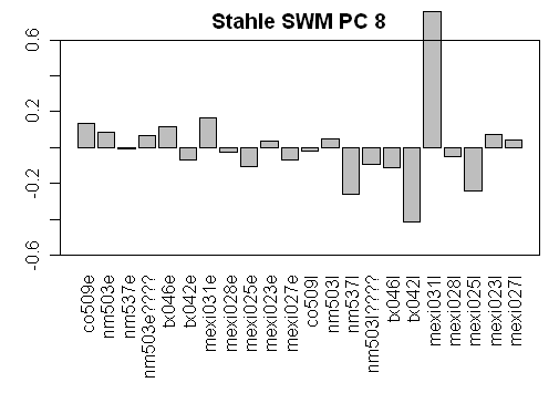
As you examine the weights of different Stahle/SWM PCs, reflect on whether MBH have successfully excluded the possibility that (say) the Stahle PC8 (or for that matter the PC3, PC2 or PC1) might simply be some local noise.
First here is a location map showing the 10 Stahle SWM sites reported in the original SI. In the Corrigendum, in response to a request for the location of an 11th site used but not listed, Mann said unhelpfully that the site was “Unpublished Southwest US/Mexico Density series (D. W. Stahle, personal communication)” – so we have no information on exactly where it is.
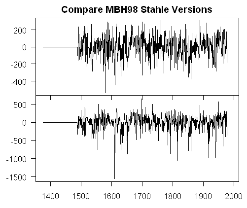
The Stahle SWM network as used in MBH98 consists of 2 series for each site – one said to be earlywood width and one said to be latewood width. The first and 11th sites have identical values for both EW and LW for the first 128 years or so, as shown in the graphic below subtracting the two series from one another. The straight line segments in the early portions denote identical values – are these different versions from the same site? Or is site 11 a different site than site 1 with values from site 1 inadvertently spliced? No one knows. When asked for an explanation, Nature refused to provide one. Obviously there’s some sort of error.
That’s tine. The insulting thing for the climate community is that the data set in Mann et al 2007 is identical to the MBH98 data set, including these obviously incorrect identical values, which remain unchanged, despite the matter being brought to Mann’s attention.
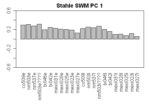
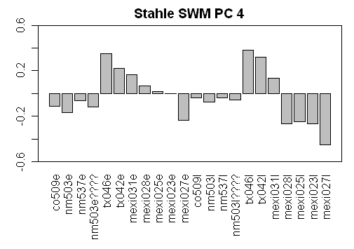
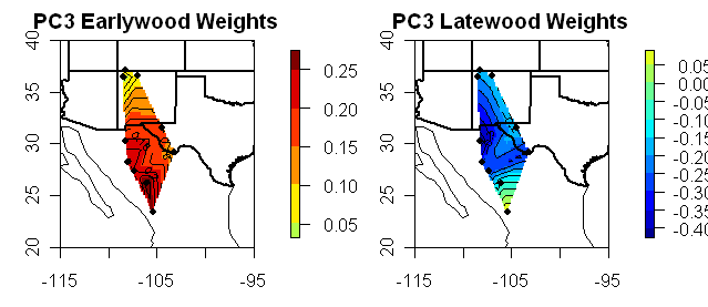
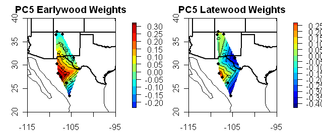
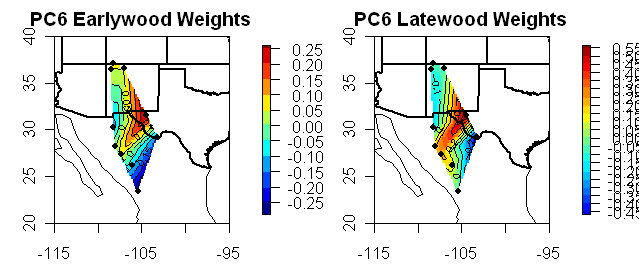
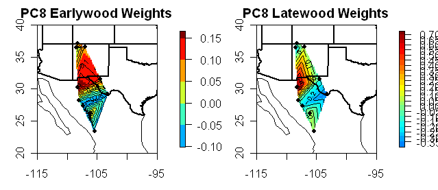
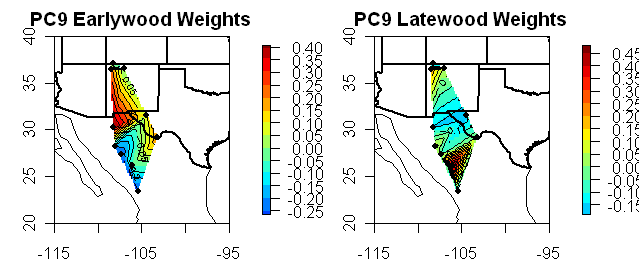
Now for a series of diagrams showing the “eigenvectors” corresponding to each PC. In every case, the eigenvectors are plausibly interpreted as weights, such that the PC1 is a weighted average and the other PCs are contrasts. First are diagrams showing the weights for each series as barplots (update: I’ve added in contour maps showing eigenvector weights separately for Earlywood and Latewood as both are reported for each site.)
First here are the weights for the PC1.
Now here are the weights for PC2-PC9, all said to be “significant”. The PC2 can be interpreted as a contrast between the sites in northern New Mexico and the sites in Texas/Mexico. The PC3 can be interpreted as a contrast between earlywood and latewood. Neither of which seem readily interpretable in terms of the top 16 world climate patterns. But it gets rapidly worse as the later contrasts and contrasts between relatively arbitrary combinations of sites and LW/EW choices. How can the contrast shown in the PC7 be plausibly linked to any world climate pattern? It is total bilge.
Mann et al said that it was “relatively unlikely” that “a proxy indicator represents a truly local climate phenomenon which is uncorrelated with larger scale climate variations”. But surely no one can seriously believe that the Stahle/SWM PC7 is anything other than some local noise. This is an extreme example – but readers should understand that the network is mostly noise. That’s why reconstructions with stocks and white noise do just as well as actual “proxies”.
And the problem is not avoided by not doing PCs. Multiple inverse regression a la MBH and Wahl and Ammann has its own very serious problems, which people have barely scratched the surface of. It’s amazing that this stuff is taken seriously.
Contour Maps
These are done using Mannomatic PCs but the effect of the Mannomatic is not large in this network.











29 Comments
Grant Foster http://www.aavso.org/news/foster.shtml has the following advice for Tamino:
D’ya think that Tamino’s ever looked at the eigenvectors of the tree ring networks? Didn’t think so. As, Grant Foster says, look at the curves.
Small word error: “That’s tine” likely meant to be “That’s fine”.
Bilge level is just a small notch above sunk. Does MBH98 have any qualities that could keep it afloat?
Wow, for lack of support is he cheering himself now.
Grant Foster = Tamino
Steve: The quote came from a house interview by AAVSO with Grant Foster http://www.aavso.org/news/foster.shtml in connection with variable stars and was about data analysis and not about his present incarnation as HAnsen’s pit bull, or in this case, as Mann’s pit bull – the latter being a beast whose ferocity would go without question.
I would say that the relationship between temperature and growth being parabolic rather than linear is in the realm of proven. Not just remotely possible conjecture.
The claim that, until proven otherwise, local temperature trends are assumed to in synch with planetary ones, is one that should be laughed out of court.
#4, It’s actually even worse – it’s the assumption in some cases that contrasts in local trends are in synch with planetary patterns i.e. that the difference between two Mexican site chronologies has a statistically significant relationship to some world “climate field.”
Yup. They should have “moved on.” Any signals in that mess are probably moisture signals, anyway.
When will you write a paper or a series of papers about all of this for a journal? Get it out there.
I’d imagine it would be a “win” either way … if it’s accepted and discussed, the scientific community will benefit, if it’s not, you can claim that the establishment is fearful of your analyses and what it may mean so they squashed it, which all the armchair analysts and commenters would eat up. Either way, it could work out well.
For those of us who don’t have the time to follow every single post and the hundreds of comments … this would be great … just sayin’. Carry on.
Is it convenient to plot the eigenvalues for the various PCs of each site on the map to reveal geographic distribution patterns (or lack thereof)? It’s been a useful technique in paleo-oceanography as shown by this example.
#7. This re-visit to proxy world has been very helpful. One of the reasons why I haven’t published on the linear algebra of these manipulations is that there were a couple of points that I was stuck on – points that one can manoeuvre around empirically but which spoiled the analysis for me. One issue was the representation of the re-scaling, which I’ve now reanalyzed and improved; the other was the representation of the weighting which I’ve now revisited and improved. My implementation of MBH is now a couple of lines of linear algebra and very pretty and is now probably worth doing though it only covers a fraction of the issues.
#8. One of the problems in doing such a plot is that there are two values for each site – EW and LW. If there were just one value, I could do this in a couple of minutes. As soon as I say this, I suppose that the logical way to show this would be to do EW and LW eigenvector maps side by side. Ill do a couple.
Steve thanks for this very informative post–it clarifies a lot for me about what the PCs mean. In normal science, you can make assumptions like tree rings are linear functions of temperature, but you are then expected to provide some rigorous test of that assumption, not build a whole world view on it and object when someone asks about that assumption. In evolutionary biology for example, someone writes a theory paper with assumptions x, y, z, but the next theory paper (or empirical one) says: “what if x does not hold?” or “does x hold?” and this progression of assumption and test has been very productive. In the climate case, the linearity assumption is completely untested and if it is false the whole house of cards crumbles. Not very robust.
The MBH quotation contains the caveat beginning:
Was there anything else in the paper that justified this assumption? This is one thing thst the reviewers should have required as essential to their assessment of the worth of the manuscript.
#8 Did up the maps and they illustrate the point rather well. I’ve done these eigenvector maps on a number of occasions. I don’t know why I didn’t think of separating the EW and LW plots before. Anyway the point is illustrated rather well.
Stahle is excellent for interdicting the SW monsoon. Generally, it will be expressed, in these region, as Easterly Waves. No matter what monsoon is doing further to the NW (e.g. variance in area affected) this part of the flow tends to be pretty consistent.
#13 – Very nice, Steve; thanks. PC1 – PC3 show north-south gradients, PC4 – PC6 show peak values in the middle, and PC7 – PC9 seem to be mixed bags. The EW and LW look fairly comparable even though the eigenvalues differ. The next exploratory thing to do is to look at the geophysical that might explain these results (not necessarily you, of course; anybody with an interest, have at it).
#15. There are some interesting articles explaining the “horseshoe” (upside down quadratic) results of biplots using PCs in ecological ordinations. Diaconis , a very big math name, has a paper slumming in this topic in which he discusses the number of changes of signs in eigenvectors for certain specialized matrices (Toeplitz) where all the columns are positively correlated (with some additional constraint). http://www-stat.stanford.edu/~susan/papers/horseshoes6.pdf
Under the conditions, each successive eigenvector has one more change of sign than the one before. Thus, the first eigenvector is sort of an average; the second one has one change of sign (a gradient), the third one has two changes of sign, … Looks like something similar may be at work here. The pattern of eigenvectors may be exactly what one expects from positively correlated sites – nothing to do with climate.
That might be quite a pretty mathematical demonstration.
Steve:
I am puzzled by the low weights derived for each proxy for each PC. Are these rotated PCs? If not, why not? Your mapping seems to have the effect of a rotation in that they highlight particular sets of variables albeit by their geography. Would rotating the PCs produce a similar set of results – in particular highlighting single factors defined by a single proxy?
I’m stunned. Surely all climate proxies represent “a truely local climate phenomenon”. If they do not, of what value are they as a proxy? Without a physical reason (the local phenomenon), surely they are nothing more than a classic spurious correlation!
But ignore that for the moment – if they somehow do represent some “global climate field”, then why go to the trouble of making sure there is good spatial coverage? You don’t need it if the proxy somehow represents a global state, rather than a local one. Of course, that would require some pretty significant evidence – that some “global signal” is captured, rather than a local one. Several decades of out of sample predictions that prove to be accurate would do, I would think. Time, once again, to “update the proxies”, methinks.
re: #18 Neil,
I believe that the theory is that the ring-widths contain a relatively high-frequency local signal, a low frequency global signal and some sort of noise of various sorts. The idea is to filter out the local signal and use the spatial coverage to attenuate the noise, assuming it will vary locally. You’re then supposed to be left with a good representation of the global signal.
Of course the team hasn’t used correct statistical methods and haven’t ever tried to justify the assumptions in the first place. So we’re left with some sort of if… then logic where nobody ever got around to the step of justifying the if and instead just asserted the then.
if A then B
maybe A (or assume A because of the precautionary principle)
Therefore B.
Dave wrote:
If that is the case, then one should – with sufficient spatial coverage – be able to do the reverse. That is to say, extract the high frequency component (which is supposed to be local only conditions) and use these to generate a global average temperature using methods similar to GISS or HADCRU. If the theory is correct then the correlation to GISS/HADCRUT etc should be reasonable, right? Does anyone know if this has been tried? Does anyone want to try and do it? (sorry, it’s beyond my skills)
#16 – This math is beyond my depth, but let me ask a simple question. Are you saying that the eigenvectors are showing that the sites are more similar to each other just because they reflect tree growth rather than responses to specific climate factors? Put another way, perhaps erroneously, is there “auto-correlation” between sites?
Craig 11
I don’t believe that it is necessary that the relationship be linear. However, it is mandatory that the relationship be monotonic, at least in the range of interest/use.
Experience and Steve’s correlation data both suggest that the growth curve is peaked (not too hot, not too cool, but just right), and it is therefore incumbent upon the users of such a “proxy” to show that it is at least locally monotonic before using it.
I think the fact that this math is so complicated and so difficult to replicate / unravel (even in Tamino’s latest post on PCAs, you can see he is struggling with replication and verification), that you have to conclude it is not the scientific method.
It is data selection to show a certain chart that the author had in mind from the beginning. Science is based on explanation and replication. This is certainly not that at all.
#23. Tamino seems to want to re-open every one of Mann’s scabs. Today he’s wading right into the Gaspé mess – he doesn’t seem to have read a single word of any of our papers.
#24: Seems like he’s not reading CA either. Who’s the first to ask Tamino more information about the “treeline11 proxy” 😉
Dave Dardinger@19
Yes, I agree that this is the central point. I accept the idea that the high frequency local signal is a function of many variables like temperature, moisture, sun light, fertilization, etc.– or maybe more accurately, it a composite signal of several high frequency signals. And I think its very reasonable to assume that there is a low frequency signal that is global (there might even be low frequency signals that are local — but lets set this aside for now).
It seems to me that the low frequency signal is also a composite signal. So to convert trees into thermometers, you would need to remove the local signal, remove the noise, and then separate the remaining signal into its component parts and select the one that represented temperature variation. I could accept such a process. But how do you know which component to select particularly if there are multiple variables of similar strength? This really isn’t a rhetorical question on my part. I’m simply wondering if there is a workable method for doing this.
Tamino, Energizer Bunny, et al … they are the Fr. Coughlin equivalents of the blogosphere, in these subject areas. Reason does not figure prominently in their world views.
re: #26 MPaul,
Hey, I was just giving the theory. I don’t agree with it for various reasons including the same reason you ask about. And while there might indeed be ways to separate out the temperature signal from other signals, I’ve not seen an example which works, and I’d think that if there were one, warmers would trot it out and make it well known.
BTW, for people wanting to be taken seriously. It’s important to be able to articulate accurately (and dispassionately) the position of those you disagree with. If you can’t do that, take a break and work on your knowledge base until you can. If you present a position which is clearly not what your opponent believes then you’ll never convince anyone in your opponent’s camp. Further you’ll cause your allies to raise their eyebrows and downgrade your reliability.
OTOH, if you do state correctly and clearly what your opponent believes, your statements of why you disagree with that position will be taken seriously.
If the data gathered by such a method didn’t support their conclusions, there’s no quarentee that they would “trot it out”. It might go into the censored directory, along with other inconvenient results.