In my post The Accidental Tourist I discussed the relationship between the Russian Meteo daily temperature record for Kurgan and two of the GHCN records for that same weather station. One surprise I learned was that GHCN discarded an entire month’s worth of data when a single data point was suspect. Doing so left GISS estimating the missing month in order to calculate an annual average.
The daily records from Meteo provide an opportunity to test the accuracy of the GISS estimation algorithm. They also give an indication as to how readily data is dropped from the record, and perhaps a little bit of hope that the accuracy of the historical record can be improved.
In the referenced post I noted that the “GISS.0” record for Kurgan was derived from the Meteo record’s “Mid” values. Furthermore, I had found that there were eleven months in the Meteo record with a single suspect daily record that caused the entire month to be dropped from the GISS.0 record. For this particular effort I started by focusing on those eleven months.
In order to compare the GISS.0 estimate with the actual Meteo record, I needed to be able to do two things.
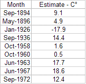
First, GISS does not record the estimated monthly value – they continue to report it as “999.9”. Instead, they record an estimate for the seasonal average and the annual average. To determine the monthly estimate I needed to have enough other data points available to reverse-calculate the monthly estimate. Of the eleven months in question, nine of them had sufficient data available for a reverse-calculation. Here are those nine months:
Second, I had to determine what value to assign, or estimate, for the suspect data points in the Meteo record. In the case of the data points I was interested in, all were flagged as having a Mid value that was either lower than the Min or higher than the Max. This fact left me with four fairly straightforward options:
- Ignore the day and calculate the average over the remaining days in the month.
- Use the Mid value anyway.
- In place of the Mid value, use the Min or Max value flagged as being inconsistent with the Mid value.
- Interpolate the value using the previous and next day Mid values.
Some may ask why I did not have a fifth option, which would be to use the mean of Min and Max. The reason is that for five of the months in question, Max values were not available.
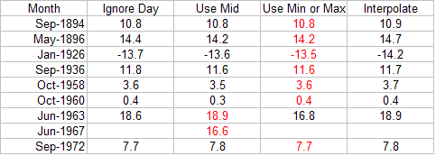
I decided to try all four options and see what the effect was on the monthly average. Here is a side-by-side comparison:
For each month, my choice as to handle the day that had the problem data is highlighted in red. Here is the rationale behind those selections:
- June 1963 – the 24th was flagged because the Mid value of 27.8 was higher than the Max value of -36.5. I concluded the sign of the Max value was transcribed incorrectly – a common error that I have seen many times in the quality control outputs from GHCN. I decided it was appropriate to keep the Mid value.
- June 1967 – no dates were flagged. I have no idea why this month was dropped from GHCN. I decided it was appropriate to keep the Mid value.
- For the remaining months, it seemed to me likely that the Min and Mid values were inadvertently swapped during transcription. Use of interpolation or simply ignoring the day altogether seemed excessive. For the most part, the difference between one method and the other was not terribly large.
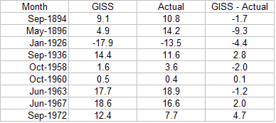
I then compared my results with the GISS estimates:
As one can readily see, the GISS algorithm did a pretty good job with October, 1960.
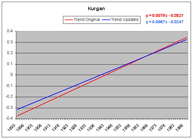
There are 1063 months in GISS.0 that have a valid (non-999.9) temperature record. It is sensible to ask whether or not adding nine more months of valid records has a material effect on the overall record. After all, those nine months affect a total of just nine years, and to a much lesser degree than the monthly effect. It is near impossible to perceive the difference when plotting the two series together, so what I did instead was plot their anomaly trends:
Thus, in the case of Kurgan (not necessarily the general case), replacing a small number of estimates with actual data reduced the slope of the warming trend a small amount.


22 Comments
Word to the wise: try not to read one of Steve’s ironic comments while drinking coffee – it goes everywhere and its a pain to clear up.
John A, I think that advice applies to John Goetz.
Also.
It didn’t change the trend very much, but the Actual versus GISS Method indicates that the GISS estimation algorithms are approximately suspect/faulty/horrible/garbage/useless.
Perhaps when all the adjustments are added, we get a distribution without added warming bias. Oh, well one CAN dream, can’t one?.
The trend changes 15%, which seems not a small amount.
Up to 9,3C difference, one start to think if their software has even entered beta testing yet.
This was probably just one station of many with a few single days missing causing the whole month to be estimated.
It would be very interesting to know how well the estimate is overall, Was this station just an odd example or are the variations this big in genreal when an estimate is done?
Going through all records and make a table of avarage estimate errors is not very easy task but it would really reveal how well the estimations work globally when only minor parts of the data is missing.
Has the performance of the estimates been checked before in those cases where most of the data is available or is it just random picks so far?
Hmm, it seems that the early values are estimated too low, whereas recent values are estimated too high. Thus contributing to increased warming trend.
Just wondering, maybe the algorithm by GISS includes the typical correction of past values to colder ones to avoid UHI effects? Therefore applying the correction twice for those values (first in the guessing of the temperaure, then in the general correction for all values)? Does the Kurgan station qualify as urban? If so, which is the correction trend they apply to its data?
And apparently there are different sets of Kurgan data from different institutions. Although there’s only one station…
Last night I looked at the two closest GISS stations to Kurgan with records on the Meteo website. These stations are Petropavlovsk and Kustanai. I applied the same ground rules for selecting months as described above. Both station records had many more additional opportunities for replacing the GISS estimate with an estimate based on actual daily records. For example, several months had one to five days missing, but valid data for all remaining days. This is unlike the Kurgan record which was all-or-nothing.
Here is a listing of the differences between the GISS estimate and the actual temperature for those months that fit the criteria above:
I did take a look at the effect on the trends for the two stations, and it is very small. In the case of Petropavlovsk, the slope of the trend does not change, but the entire trendline is translated downward by 0.01 degrees. The change to Kustanai’s trend line is similar to Kurgan, but to a much smaller extent (about 1/10th).
I just noticed that the Meteo ftp directory is now empty, and was modified today.
John,
What about GISS (and NOAA) using an equal month weighting vs. a number of days weighting (both with and w/o leap years)? Both for annual temp varation and for annual trend.
Re: #5
After reading the various analysis on temperature reading on this site (from changes in methods in measuring sea temps to ‘adjustments’)one wonders what the record might look like without all the point shaving. While the general trendline would not change (or so I suspect) it gives one pause to think that GCM’s and proxy calibrations to instrumented data would then be off – but then what would that say about GCM robustness?
Joe, that’s an interesting question. I doubt it amounts to much but is easy enough for me to calculate with what I have. I will look at it later tonight.
12 (JohnG)
The ftp Meteo directory was empty yesterday already – I’ve looked.
RE 15
Sure it’s minor, but this supossed to be SCIENCE. Access to computers has been available to SCIENCE since the 60’s if not the 70’s. Computers to the people since the 90’s (arguably the 80’s).
Using a daily weighting would seem to be the “right thing to do”, and certainly not beyond the capabilities of available hardware.
Engineering shifts to Science at somewhere between 10% and 1% of point. Engineering Safety Factors have shifted from 10x (Hoover Dam) to approx 1.1x these days.
The GISTEMP anomaly trend is less than 6% of the nominal 14 it’s based off of. If this trend is off 15%, what does that say.
Now, let’s see how the “trend” changes when one takes all of the “adjustments” to the temperature record out. Can this be done? Have all of the temperature “adjustments” been recorded and have they been justified?
The contemporaneous “adjustments” to the PAST record, that is.
#19 Gaelen: Presumably, the data I am working with is raw, unadjusted data.
#17 Joe … I did a quick run on one of the Russian stations I had not yet looked at. That is, I calculated the annual average the way GISS does: first calculate monthly averages, then calculate seasonal averages from the three monthly averages, then calculate annual average from the four seasonal averages. Then I calculated the annual average a second way: simply take all days in the year and calculate the mean at once.
I had assumed the difference between the two methods was small. I was wrong. For the single station I examined it was substantial, ranging from -1.11 C to +0.87C.
I have Meteo data from four other stations. I want to go through those before I make any general conclusions.
One Trackback
[…] May I began a quest to better understand how GISS does its homogeneity adjustment, also known as GISS Step 2. Steve McIntyre took the ball from that scrum and ran with it, producing […]