Detroit Lakes in BEST

In the 2007 analysis of the GISS dataset, Detroit Lakes was used as a test case. (See prior posts on this station here). I’ve revisited it in the BEST data set, comparing it to the older USHCN data that I have on hand from a few years ago.

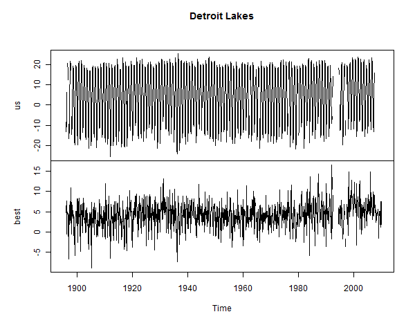
First, here is a simple plot of USHCN raw and BEST versions. The BEST version is neither an anomaly series (like CRU) nor a temperature series (like USHCN). It is described as “seasonally adjusted”. The mechanism for seasonal adjustment is not described in the covering article. I presume that it’s somewhere in the archived code. The overall mean temperature for USHCN raw and Berkeley are very close. The data availability matches in this case – same starting point and same gaps (at a quick look). So no infilling thus far.

Figure 1. Simple plot of USHCN Raw and BEST versions of Detroit Lakes

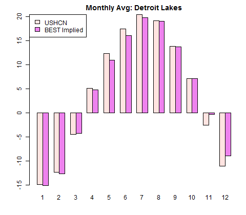
The Berkeley series is not, however, the overall average plus an anomaly as one might have guessed. Here is a barplot comparing monthly means of the two versions. While the Berkeley version obviously has much less variation than the observations, it isn’t constant either (as it would be if it were overall average plus monthly anomaly). I can’t figure out so far where the Berkeley monthly normals come from.

Figure 2. Monthly Averages of two versions.

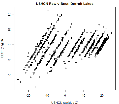
If one does a simple scatter plot of USHCN raw vs Berkeley, one gets a set of 12 straight lines with near identical slope, one line for each month:

Figure 3. Scatter plot of USHCN raw vs Berkeley

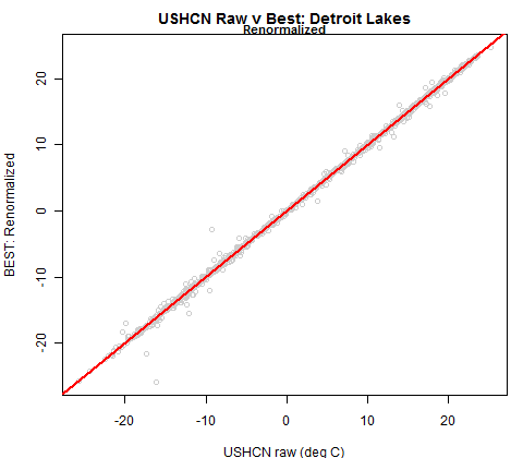
I then tried the following. I subtracted the Berkeley monthly average from each Berkeley data point and added back the USHCN monthly average. This yielded the following:

Figure 4. USHCN raw versus Berkeley (renormalized for each month)

The Berkeley data seems to be virtually identical to USHCN raw data less monthly normals that are different from normals of USCHN raw data plus annual average. The implied monthly averages in the BEST normalized data are shown below. The range of difference is from -2.27 to 1.41 deg C.

My original examination of Detroit Lakes and other stations was directed at whether NASA GISS had software to detect changes – a point that had been then been raised in internet debates by Josh Halpern as a rebuttal to the nascent surface stations project. I used Detroit Lakes as one of a number of type cases to examine this, accidentally observing the Y2K discontinuity. One corollary was that GISS software did not, after all, have the capability of detecting the injected Y2K discontinuity.

It would be interesting to test the BEST algorithm against the dataset with the Y2K discontinuity to see if they can pick it up with their present methodology. At first blush, it looks as though USHCN data is used pretty much as is, other than the curious monthly normals.

[Update: it looks like this data is prior to homogenization.]

This entry was written by Stephen McIntyre, posted on Oct 29, 2011 at 2:53 PM, filed under Uncategorized and tagged best, detroit lakes, nerkeley. Bookmark the permalink. Follow any comments here with the RSS feed for this post. Both comments and trackbacks are currently closed.

13 Comments

Steve McIntyre

Posted Oct 29, 2011 at 3:10 PM | Permalink

#BEST
	load("d:/climate/data/berkeley/details.tab")
	load("d:/climate/data/berkeley/station.tab")
	detailsb=details
	detailsb[grep("DETROIT L",detailsb$name),1:5]
# 144289 144289 DETROIT LAKES(AWOS) 46.8290 -95.8830 425.500
#144298 144298 DETROIT LAKES 1 NNE 46.8335 -95.8535 417.315

#USHCN
	load("d:/climate/data/station/ushcn/200802/ushcn.collation.tab")
	us=ushcn.collation$raw
	load("d:/climate/data/station/ushcn/details.tab")
	detailsu=details
	detailsu[grep("DETROIT L",detailsu$name),1:5]
#       id   ghcnid               name state division
#444 212142 72753004 DETROIT LAKES 1NNE    MN        1

#COMBO
	trim=function(x) window(x, start=min (time(x)[!is.na(x)]), end= max (time(x)[!is.na(x)]) )
	X=ts.union(us=trim(us[,paste(212142)]),best=station[[paste(144298)]])
	tsp(X) # 1895.000 2009.917 
	month= factor(rep(1:12,nrow(X)/12) )
	Avg=cbind( us=unlist(tapply(X[,1],month,mean,na.rm=T)),
	  best=unlist(tapply(X[,2],month,mean,na.rm=T)) )
	Avg
 	#          us     best
	#1  -14.888840 4.369898
	#2  -12.400299 4.459945
	#3   -4.509250 3.857273


png("d:/climate/images/2011/berkeley/detroitl_ts.png",w=600,h=480)
	par(mar=c(4,4,2,1))
	plot.ts(X[,1:2],,main="Detroit Lakes")
dev.off()



png("d:/climate/images/2011/berkeley/detroitl_barplot.png",w=480,h=420)
par(mar=c(4,4,2,1))
	barplot (t(Avg),beside=TRUE,col=c("mistyrose","violet") )
	title("Monthly Avg: Detroit Lakes")
	legend("topleft",fill= c("mistyrose","violet") ,legend=c("USHCN","BEST") )
dev.off()

#Show comparison
	X=data.frame(X)
	X$avgb=X$avgu=month
	levels(X$avgb)= Avg[,"best"]
	levels(X$avgu)=Avg[,"us"]
	for(i in 3:4) X[,i]=as.numeric(as.character(X[,i]))
	X$fix=X$best-X$avgb+X$avgu

png("d:/climate/images/2011/berkeley/detroitl_scatter1.png",w=480,h=420)
	par(mar=c(4,4,2,1))
	plot(X$us,X$best,xlab="USHCN raw(deg C)", ylab="BEST (deg C)")
	title("USHCN Raw v Best: Detroit Lakes")
dev.off()


png("d:/climate/images/2011/berkeley/detroitl_scatter2.png",w=480,h=420)
	par(mar=c(4,4,2.2,1))
	plot(X$us,X$fix,xlab="USHCN raw (deg C)", ylab="BEST: Renormalized",col="grey80")
	abline(0,1,col=2,lwd=2)
	title("USHCN Raw v Best: Detroit Lakes")
	mtext(side=3,line=0,cex=.9,font=2,"Renormalized") 
dev.off()


Avg=cbind(Avg, Avg[,1]- (Avg[,2]-4.13))
png("d:/climate/images/2011/berkeley/detroitl_barplot2.png",w=480,h=420)
par(mar=c(4,4,2,1))
	barplot (t(Avg[,c(1,3)]),beside=TRUE,col=c("mistyrose","violet") )
	title("Monthly Avg: Detroit Lakes")
	legend("topleft",fill= c("mistyrose","violet") ,legend=c("USHCN","BEST Implied") )
dev.off()

GaryW

Posted Oct 29, 2011 at 3:32 PM | Permalink

Steve,
As near as I can tell, the BEST seasonal normalization contains a 4 month period oscillation. Third harmonic ringing in their low pass filter?

Steve: no idea. I’m starting with their results and observing properties.
WillR

Posted Oct 29, 2011 at 4:59 PM | Permalink

For anyone who has trouble on Windows…

Lines that look like this — change the quotes…
load(“d:/climate/data/berkeley/details.tab”)

To this:
load(“d:/climate/data/berkeley/details.tab”)
Straight Upsy-downsy Quotes…

There are quite a few to change — in the plot lines (which are thickening — sorry couldn’t resist…)

I also moved the “details,tab” to the directory you referenced
load(“d:/climate/data/station/ushcn/details.tab”)

Presumably it was the same “details.tab” we downloaded previously…

At least I duplicated your graphs… fwiw So I am guessing I was correct…

Next?
- WillR
  
  Posted Oct 29, 2011 at 5:00 PM | Permalink
  
  And now I see it is WordPress –FIXING the quotes… argghhh!
  
  Steve: There’s a command in wordpress to block off the text. Pete holzman knows the command. I’ll try to locate it.
  - hro001
    
    Posted Oct 29, 2011 at 6:03 PM | Permalink
    
    You could try <pre> </pre> … not sure how that will come through … but here’s a test (works in a post, so, at least in theory, it should work in a comment:
```
title("USHCN Raw v Best: Detroit Lakes")
mtext(side=3,line=0,cex=.9,font=2,"Renormalized")
```
    Steve: Thanks, Hilary. That’s what I wanted.
  - hro001
    
    Posted Oct 30, 2011 at 12:37 AM | Permalink
    
    Steve: Thanks, Hilary. That’s what I wanted
    
    You’re most welcome, Steve. Your usage of this Helpful Hint from Hilary™ gives me confidence to grant myself a brownie point for my (very minor) contribution to the advancement of understanding BEST 😉

BillC

Posted Oct 29, 2011 at 3:38 PM | Permalink

I don’t have the USHCN data (yet, here) as I just started with BEST. The BEST data contains a record for #samples in each monthly record at each station. Generally these seem to be daily – e.g. the one for the Detroit Lakes station above averages just over 29 samples per record when the field isn’t null (-99). Is this typical of the underlying dataset (daily records)?

Steve – I have an old but relevant USCHN collation online at http://www.climateaudit.info/data/station/ushcn/
- BillC
  
  Posted Oct 29, 2011 at 5:16 PM | Permalink
  
  thx got it
Willis Eschenbach

Posted Oct 29, 2011 at 7:18 PM | Permalink

Steve, have they released the raw data (as opposed to the “seasonally adjusted” data) yet? I find it frustrating to use data that’s been pre-munged …

w.

Steve: there ‘s a very large file of original data. It was too large for my computer to read. Much of it will probably be the same as GHCN.
- TerryMN
  
  Posted Oct 29, 2011 at 8:23 PM | Permalink
  
  Kinda sorta related to the “too large for my computer…” – Oracle is now supporting R in the database – I’m hoping to get some time on an Exadata to push it… 😀
  
  info – http://www.oracle.com/technetwork/database/options/odm/oracle-r-enterprise-oow11-517498.pdf
Bruce

Posted Oct 30, 2011 at 11:57 AM | Permalink

What is the data (Steve supplied) from BEST actually describing? I looked at my home town (the years were right).

The first 4 months:

BEST: 8.892 8.109 8.241 7.421

Environment Canada Mean: 2.6 2.3 4.5 6.4

Environment Canada Max: 6.5 6.8 10.1 11.6
GaryW

Posted Oct 30, 2011 at 10:10 PM | Permalink

Steve,
If you don’t mind a little amateurish work, I done a quick writeup of my examination of BEST data for my town. I was careful to use only the simplest manipulation of data so as to preserve as much of its original content as practical. I am not impressed with the quality of the work from BEST.

Click to access BEST_data_for_Lebanon_Missouri.pdf

Gary Wescom
WillR

Posted Oct 31, 2011 at 10:31 AM | Permalink

For those who want to follow the R Discussions but need a quick course or refresher… I am going to suggest the Andrew Robinson documents as they seem to bring you along fairly rapidly…

Just click on this link:
http://www.ms.unimelb.edu.au/~andrewpr/

The go to the R-Users group directory to download his notes and data. There are a few quirks to entwrig the listings — but that’s all..

Start a new edit window, then just cut and paste from the book and remove the chevrons “>” and the Pluses “+” from the beginning of each line when you paste — that should do it.. The “Select and Execute”…

You can continue to add to a script and just execute the new part using the “Edit” menu — “Run Line or Selection”..

Then save the script at appropriate points and carry on with the lessons.

2 Trackbacks

By Pre-Prints and Pre-Data | Watts Up With That? on Nov 1, 2011 at 4:47 PM

[…] release was not even the raw data. It was processed by removing the monthly averages … but we don’t know what those averages were, or how they were […]
By Detroit Lakes in BEST « Bee Auditor on Nov 7, 2011 at 6:37 PM

[…] Source: https://climateaudit.org/2011/10/29/detroit-lakes-in-best/ […]

Climate Audit