As many readers have already surmised, the “GCM-Q” model that visually out-performed the Met Office CMIP5 contribution (HadGEM2) originated with Guy Callendar, and, in particular, Callendar 1938 (QJRMS). My attention was drawn to Callendar 1938 by occasional CA reader Phil Jones (see here and cover blog post by co-author Ed Hawkins here.) See postscript for some comments on these articles.
Callendar 1938 proposed (his Figure 2) a logarithmic relationship between CO2 levels and global temperature (expressed as an anomaly to then present mean temperature.) In my teaser post, I used Callendar’s formula (with no modification whatever) together with RCP4.5 total forcing and compared the result to the UK Met Office’s CMIP5 contribution (HadGEM2) also using RCP4.5 forcing.
In today’s post, I’ll describe Callendar’s formula in more detail. I’ll also present skill scores for global temperature (calculated in a conventional way) for all 12 CMIP5 RCP4.5 models for 1940-2013 relative to simple application of the Callendar formula. Remarkably, none of the 12 GCM’s outperform Callendar and 10 of 12 do much worse.
I’m not arguing that this proves that Callendar’s parameterization is therefore engraved in stone. Callendar would undoubtedly have been the first to say so. It is undoubtedly rather fortuitous that the parameters of Callendar’s Figure 2 outperform so many GCMs. The RCP4.5 forcing used in my previous post included an aerosol history, the provenance of which I have not parsed. I’ve done a similar reconstruction using RCP4.5 GHG only with a re-estimate of the Callendar parameters, which I will show below.
Guy Callendar
Guy Callendar (see profile here) seems entirely free of the bile and rancor of the Climategate correspondents that characterizes too much modern climate science.
Callendar’s life got off to a good start in 1898: he was born in Canada (though he was raised and lived in England). (The next major AGW figure, Gilbert Plass, was born and brought up in Canada, though he later moved to the U.S.) He was the son of a prominent physicist, Hugh Callendar, who was succeeded at Montreal’s McGill University by Ernest Rutherford. Hugh Callendar appears to have been very prominent in his day and, among other activities, had developed steam tables that were widely used in industry. (Much of the present profile is drawn from here.)
Guy Callendar lost one eye in a childhood accident, but nonetheless was a keen tennis player, reaching the finals of the club singles championship in 1928 at Ealing Lawn Tennis Club and winning the club doubles championship at Horsham Lawn Tennis Club at the age of 49 in 1947. Not easy for someone with only one eye.
Callendar earned a certificate in Mechanics and Mathematics in 1922 at City & Guilds College and then went to work for his father examining the physics of steam until his father’s death in 1930. In 1938, Callendar was employed as a “steam technologist” by the British Electrical and Allied Industries Research Association and his seminal 1938 paper was therefore communicated to the Royal Meteorological Society by Dr G.R. Dobson, F.R.S:
Although Callendar’s qualifications would undoubtedly lead a modern Real Climate or Skeptical Science reader to dismiss him as suffering from Dunning-Kruger syndrome, Callendar (1938) is the first article that provides a clear scientific basis for modern AGW theory, albeit of a low-sensitivity and unhysterical type. Callendar’s detailed and first-hand technical expertise on steam and water vapour enabled him to articulate the infrared properties of increased carbon dioxide in the atmosphere, an understanding that appears to have eluded the contemporary establishment, whose views seem related to modern skydragons. Indeed, the structure of Callendar (1938) includes a discussion of issues that frequently trouble newcomers to the debate (spectral overlap, CO2 dissolution in the ocean) and, in my opinion, IPCC reports are diminished by not including modern reviews of such topics.
Callendar’s “Formula”
In Figure 2 of Callendar (1938) – see below, Callendar showed his estimate of the change in temperature (as an anomaly) arising from varying CO2 levels in “temperate” zones. Although Callendar did not characterize the curve in this figure as logarithmic, it obviously can be closely approximated by a log curve, as shown by the red overplot which shows a log curve fitted to the Callendar graphic. Its 2xCO2 sensitivity is 1.67 deg.
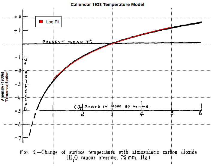
Figure 1. Callendar 1938 showing temperature zone relationship. Log curve (red) fitted by digitizing 13 points on the graphic and fitting a log curve by regression: y= -2.635113 + 2.410493 *x. This yields sensitivity of 2.41 *log(2) = 1.67 deg.
Callendar did not show corresponding graphics for tropical or polar regions, but commented that the results for other zones were similar. Nor did Callendar show the derivation of his results in Callendar (1938). It is my understanding that he derived these results from his knowledge of the infrared properties of carbon dioxide and water vapour (and not by curve fitting to observations, though he had also carried out his own estimates of changes in global temperature.)
Callendar implicitly discounted the arguments for substantial positive feedbacks on initial forcing that characterize subsequent GCMs, observing the nagative feedback from clouds as follows:
On the earth the supply of water vapour is unlimited over the greater part of the surface, and the actual mean temperature results from a balance reached between the solar ” constant ” and the properties of water and air. Thus a change of water vapour, sky radiation and tempcrature is corrected by a change of cloudiness and atmospheric circulation, the former increasing the reflection loss and thus reducing the effective sun heat.
“GCM-Q”
Although Callendar (1938) included projections of future carbon dioxide emissions and levels, Callendar had no inkling of the astonishing economic development of the second half of the 20th century. As Gavin Schmidt has (reasonably in this case) observed in connection with Hansen’s Scenario A, the ability to forecast future emissions is unrelated to the evaluation of the efficacy of a model’s ability to estimate temperature given GHG levels.
I thought that it would be an interesting exercise to see how Callendar’s 1938 “formula” applied out-of-sample when applied to observed forcing and compare it to the UK contribution to CMIP5 (HadGEM2), which I had been discussing. For my comparison, I used IPCC RCP4.5 forcing as a mainstream estimate, inputting their “CO2 equivalent” of all forcings (RCP4.5 column 2). It turns out that RCP4.5 column 2 “CO2 equivalent” includes aerosols converted to ppm CO2 somehow, as well as the other GHG gases (CH4, N2O, CFCs etc) plus aerosols (converted to ppm CO2). At present, I don’t know how these estimates have been constructed and make no comment on their validity: for this exercise, I am merely taking them as face value for a relatively apples-to-apples comparison.
Callendar’s relationship was based on anomaly to “present mean temperature”. For my calculations, I adopted the 1921-1940 anomaly as an interpretation (differences from this are slight) and therefore centered HadCRUt4 observations and HadGEM2 on 1921-40 for comparison.
Callendar’s Figure 2 is for “temperate” zones but he reported that the relationship was “remarkably uniform for the different climate zones of the earth”. For the purpose of the exercise, I therefore used the relationship of Callendar’s Figure 2 to estimate GLB temperature, recognizing that the parameters of this figure would only be an approximation to Callendar’s GLB calculation. I have not examined whether the Callendar formula might work better or worse for 60S-60N, as, in carrying out the exercise, I was not taking the position that the parameters in the Callendar formula were “right” – only seeing what would result.
Here’s what resulted (as I showed in the previous post). A reconstruction from the Callendar 1938 formula applied to RCP4.5 CO2 equivalent seemingly out-performed the HadGEM2 GCM. While some readers presumed that “GCM-Q” must have incorporated some knowledge or information of second-half 20th century temperature history in the development of the “model”, this is not the case. “GCM-Q” directly used the formula implicit in Callendar 1938 Figure 2. (I realize that my interest in the results arises in large part from their coherence with subsequent observations, but it wasn’t as though I foraged around or did multiple experiments before arriving at the results that I showed here, the first runs of which I sent to Ross McKitrick and Steve Mosher.)

Figure 2. Temperature estimate using Callendar relationship versus HadGEM2.
Skill Scores
Next in today’s post, I will quantify the visual impression that “GCM-Q” outperformed HadGEM2 by using a skill score statistic that is commonplace in the evaluation of forecasts, estimating the “skill” of a model from the sum of squares of the residuals from the proposed model as opposed to a base case, as expressed below where obs is a vector of observations and “model” and “base” are vectors of estimates.
skill = 1 - sum( (model-obs)^2)/sum( base-obs)^2)
This calculation is closely related to the RE statistic in proxy reconstructions, where the base case is the mean temperature in the calibration period. However, the concept of a skill score is more general and long preceded the use of RE statistics in proxy reconstructions. In today’s calculation, I used 1940-2013 for comparison (using 2013 YTD as an estimate of 2013.)
In addition to calculating the skill score of HadGEM2, I also calculated skill scores for the 12 CMIP5 RCP4.5 averages on file at KNMI. These skill scores (perfect is 1) are shown in the barplot below:
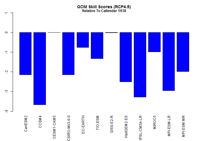
Figure 2. Skill Scores of CMIP5 RCP4.5 models relative to Callendar 1938.
Remarkably, none of the 12 CMIP5 have any “skill” in reconstructing GLB temperature relative to the simple GCM-Q formula. Indeed, 10 of 12 do dramatically worse.
Aerosols
In the comments to my previous post, there was some discussion about the importance of aerosols and whether 20th century temperature history could be accounted for without invoking aerosols.
Directly using the Callendar 1938 “formula” on RCP4.5 GHG CO2 equivalent (RCP column 3) leads to a substantial overshoot of present temperatures. As an exercise, I re-calibrated a Callendar-style logarithmic relationship of temperature to RCP4.5 GHG and did the corresponding reconstruction of 20th century temperature history, once again calculating skill scores for each of the CMIP5 GCMs, this time against the Callendar-style estimate only using GHG (no aerosols), as shown in the graphic below:
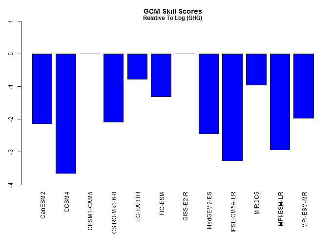
Figure 3. Skill Scores of CMIP5 RCP4.5 models relative to re-calibrated Callendar-style estimate using GHGs only.
The temperature reconstruction using the reparameterization is shown in the graphic below. This reconstruction is not out-of-sample, as observations have been used to re-calibrate. Its climate sensitivity is lower than the Callendar 1938 model: it is 1.34 deg C.
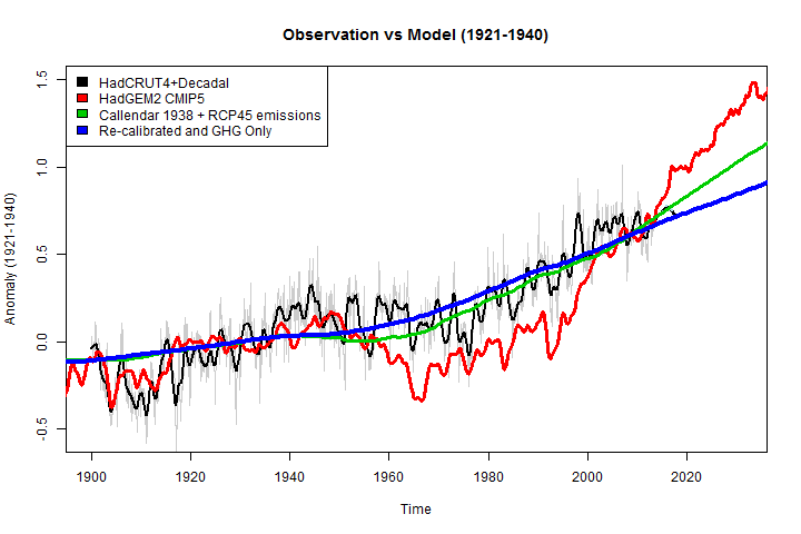
Figure 4. As Figure 2 above, but including recalibrated temperature reconstruction using RCP4.5 GHG (column 3).
Comments
What does this mean? I’m not entirely sure: these are relatively new topics for me.
For sure, it is completely bizarre that a simple reconstruction from Callendar out-performs the CMIP5 GCMs – and, for most of them, by a lot. For the purposes of this observation, it is irrelevant that Callendar reconstructed temperature zones (both given his comment that other zones were remarkably similar and the fact that the specific parameters of Callendar Figure 2 are not engraved in stone). Even if the Callendar parameters had been calculated using the observed temperature history, it is surely surprising that such a simple formula can out-perform the GCMs, especially given the enormous amount of time, resources and effort expended in these GCMs. And, yes, I recognize that GCMs provide much more information than GLB temperature, but GLB temperature is surely the most important single statistic yielded by these models and it is disquieting that the GCMs have no skill relative to a reconstruction using only the Callendar 1938 formula. As Mosher observed in a comment on the predecessor post, a more complicated model ought to be able to advance beyond the simple model and, if there is a deterioration in performance, there’s something wrong with the model.
From time to time, others have pointed out this ability of simple models (and a couple of readers have sent me interesting essays on this topic offline). In one sense, “GCM-Q” is merely one more example. However, the fact that the parameters were estimated in 1938 adds a certain shall-we-say piquancy to the results. Nor do I believe that one can ignore the relative coherence of Callendar’s low sensitivity results to observations in forming an opinion on the still highly uncertain issue of sensitivity. That GCM-Q performed so well out of sample would interest me if I were a climate modeler.
Third, all the GCMs that underperform the Callendar formula run too hot. It seems evident to me (and I do not claim that this observation is original) that the range of IPCC models do not fully sample the range of physically possible or even plausible GCMs at lower sensitivities. Perhaps it’s time that the climate community turned down some of the tuning knobs.
Finally, Callendar 1938 closed with the relatively optimistic comment that, in addition to the direct benefits of heat and power, there would be indirect benefits at the northern margin of cultivation, through carbon dioxide fertilization of plant growth and even delay the return of Northern Hemisphere glaciation:
it may be said that the combustion of fossil fuel, whether it be peat from the surface or oil from 10,000 feet below, is likely to prove beneficial to mankind in several ways, besides the provision of heat and power. For instance the above mentioned small increases of mean temperature would be important at the northern margin of cultivation, and the growth of favourably situated plants is directly proportional to the carbon dioxide pressure (Brown and Escombe, 1905): In any case the return of the deadly glaciers should be delayed indefinitely.
This last comment was noted up in Hawkins and Jones 2013, who sniffed in contradiction that “great progress” had subsequently been made in determining whether warming was “beneficial or not”, bowdlerizing Callendar by removing Callendar’s reference to direct benefits (heat and power) and carbon dioxide fertilization:
Since Callendar (1938), great progress has been made in understanding the past changes in Earth’s climate, and whether continued warming is beneficial or not. In 1938, Callendar himself concluded that, “the combustion of fossil fuel [. . .] is likely to prove beneficial to mankind in several ways” , notably allowing cultivation at higher northern latitudes, and because, “the return of the deadly glaciers should be delayed indefinitely”.
Postscript
As noted above, my attention was drawn to Callendar 1938 by occasional CA reader Phil Jones in Hawkins and Jones (2013) (here), which was discussed by coauthor Hawkins here.
Hawkins and Jones (2013) focused on one small aspect of Callendar’s work: his compilation of World Weather Records station temperature data into zonal and global temperature anomalies, in effect, delimiting Callendar, whose contribution was much more diverse, as a sort of John the Baptist of temperature accountancy, merely preparing the way for Phil Jones.
They noted that Callendar was “meticulous” in his work, an adjective that future historians will find hard to apply to present-day CRU. Hawkins and Jones observed that Callendar’s original working papers and station histories had been carefully preserved (at the University of East Anglia). The preservation of Callendar’s original work at East Anglia seems all the more remarkable given that Jones’ CRU notoriously reported that it had failed to preserve the original CRUTEM station data supposedly because of insufficient computer storage – an excuse that ought to have been soundly rejected by the climate community at the time, but which seems even more laughable given the preservation of Callendar’s records.
Postscript2: “Were Callendar’s Estimates Accurate?” is in the background to Richard Allen’s pod-snippet linked by Bishop Hill here. The screenshot in the background appears to be from the poster presentation by Hawkins and Jones – an odd choice of background.


225 Comments
Ha. Your fans are a broad church indeed.
Steve: In the previous post, I described Jones as “a CA reader, who has chosen not to identify himself at CA”. However, Jones made numerous references to CA in the Climategate dossier – thus at least an “occasional CA reader”, though arguably not a “fan”:)
I promise I won’t do this again until I at least finish the article but
has to be one of the great lines of Climate Audit history. As an obvious fellow-sufferer with Callendar I’m well pleased.
Unfortunate that Callendar correlate better false data. The only sound observational basis is satellites since 1979 and it is much too short to draw conclusions. Oddly enough, HadGEM2 CMIP5 follows a little better that HadCRUT4 what is known about surface temperatures by proxies. The cooling of the 60s and 70s is indeed the feature of the twentieth century the most characteristic and the best established.
You can find it at
http://www.biokurs.de/treibhaus/literatur/callendar/callendar1938.doc
The 1940 and 1958 papers are available by changing the date. This is from an archive put together by Ernst Beck and does not appear to be accessible through the main website.
Steve M,
Very entertaining, BUT…
Let me introduce three definitions to avoid future confusion.
The Equilibrium Climate Sensitivity (ECS) is defined (by the IPCC) as the steady-state SAT temperature achieved after a doubling of CO2.
The Transient Climate Response (TCR) is defined (by the IPCC) as the SAT temperature at the point of doubling CO2 when carrying out a 1% per year CO2 growth (numerical) experiment.
The Effective Climate Sensitivity is the apparent climate sensitivity per unit forcing expressed in degrees C per W/m2 obtained by taking the inverse slope of a plot of outgoing flux vs SAT temperature.
I have not been able to access an original version of the 1938 Callendar paper – only various other papers which reference it – so my comment here may be completely erroneous. That said, it seems that Callendar took a number of different assumed levels of CO2 and then calculated the steady state surface temperature which he thought would result from that level of CO2. This is not the same as the transient temperature which would result at the achievement of that particular level of CO2, since this is dependent on growth rate and system response time. Hence, his calculation of ECS in modern parlance was 1.67 deg C (for a doubling of CO2).
From that you can calculate a linearised effective climate sensitivity of 1.67/3.7 deg C per W/m2, or alternative if the effective forcing value is not equal to 3.7 W/m2. Using this effective climate sensitivity, you can then predict temperature from the CO2 level at a particular point in time, (converted to forcing as per your log formula). To do this, however, you also have to postulate a system response time – a missing variable here.
What I think you have done is misapplied his formula as though it yields a correct transient temperature response when the CO2 level is (arbitrarily) growing. If his formula is indeed a steady-state solution, then his actual temperature prediction would be lower.
Steve: see Callendar 1938 . Callendar did not turn his mind to transient vs steady state response. I did an experiment using the relationship in Figure 2. The outperformance of the GCMs using this simple formula is true regardless of how one interprets the transient vs steady state response. Nonetheless , I take your point that the characterization of the climate sensitivity of the formula does depend on the time path if there are material delays between forcing and temperature impact. It’s not a topic that I’ve parsed. As I recall, Lindzen argues for very short delays – a point that seems logically distinct from other issues in controversy, but I haven’t followed the arguments for and against.
.
The paper is available at http://onlinelibrary.wiley.com/doi/10.1002/qj.49706427503/pdf It seems to have been made open access.
It would be interesting to get Lindzen’s reaction on that specific point and the rest of the post. But looking good, SteveM/GuyC 🙂
Paul_K, I suspect that Callendar used logic to deduce that the difference in timescale between a transient response and final steady state in response to an increase in the steady state energy influx was less than one year.
This logical deduction is based on the fact that there is nowhere on the Earths surface where the difference in the summer maximum and winter minimum temperatures is less than any temperature change resulting from the addition of ‘green house gasses’.
It is actually rather easy to calculate the transient response, just take a thermometer and stopwatch to a place on Earth just before a total solar eclipse. You will note a drop in temperature occurs as soon as you are in the penumbra and a rapid drop when in the umbra.
DM, you’re talking here only about atmospheric response, while the argument for lags is mostly based on oceans.
I’ve taken a quick look at some energy-balance articles on the topic. One line of argument seems to be that a very slow exchange between surface and deep ocean means that the response of the surface layer to additional forcing will be rather rapid since deep diffusion is slow. Since this is the layer that is relevant for HadCRUT, this would argue for short response in the temperature measurements.
Not to venture off topic, but here is the temperature profiles at a mid-latitude site in the Northern Hemisphere (50 N, 145 W).
http://www.astr.ucl.ac.be/textbook/chapter1_node11.html
Background here
http://www.astr.ucl.ac.be/textbook/chapter1_node11.html
You can see that there is almost 10 degrees of temperature change in the top 25 meters. The lag in temperature change and light flux is about three months.
Ah the age old question of how to account for the “heat in the pipeline”. Steve’s implementation of Callendar’s formula is somewhat like a one-box model with a fast tau. To me, this model seems to fit observations better than the fast-slow reponse model of GCM’s. Not that the GCM’s agree on how fast and slow the reponse should be.
Based on some calculations I’ve done the following exponential decay model will produce a .995 R^2 statistic of the CMIP5 multi-model mean RCP4.5 scenario over the period 1900-2100:
ecs * forcing anomaly/3.7 * exp(-(t^1/2)/tau)
So essentially a one-box model using the square-root of time.
JMO, but lately I question that GHG effects have any significant time-lag. No GHG back-radiation can penetrate water beyond a few mm, unlike solar shortwave. So their “warming” effect would be almost instantaneous as SST and added atmospheric water vapor. OTOH, some of the changes in solar radiation (albedo changes) would be “stored” below the water surface & would result in a time-lag.
Quite remarkable really. If these results stand up to the white hot glare of scrutiny that will undoubtedly follow from the ‘climate community’ and do not turn out to be anything other than coincidental, this will be the most remarkable example of any scientific field which has regressed over such a remarkably long period.
Grant/funding corruption in action?
I agree with all that the fact that this old school model outperforms so many modern ones is remarkable. However I don’t find it surprising at all, and could have easily predicted that all the modern models would be running hotter without needing Steve to prove it, although I am glad he has.
As climate is the focus of this blog, it is understandable that readers feel that this scientific “regression” may be unique to climate science, but rest assured, it isn’t. There have been true believers gnawing away at other fields for decades too – economics, psychology and others too.
Tom Desabla:
A suggestive way of putting it, because for any software engineer worth his salt what Steve has shown beyond doubt is that climate science, not least its authoritative expressions in IPCC reports, has been atrocious in regression testing of its central general circulation and other models, taking that important term in its broadest and most important sense.
I can’t speak for psychology, as my therapist would surely confirm, but on economics I’m with srp‘s excellent post on Bishop Hill three days ago. Despite all its conflicts of interest the dismal science surely does a better job at maintaining some integrity than the puffed-up one for which Guy Callendar was such an excellent but neglected pioneer. Not of course that this is setting the bar higher than Lilliputian.
snip – overdeditorialzing
Tom: Thanks. My advice is never to interpret use of the Zamboni as your thoughts being “less than welcome,” just that the editor felt they weren’t right for a particular thread. There have been useful analogies made between climate and the credit crunch that I have seen and been involved in but they don’t happen all the time.
The concern at the moment is about regression testing. This should have been done all along (as Steve is effect putting right very belatedly now) and reported all along, most of all in the IPCC reports. That there is nothing is quite simply a gaping hole in the whole story. That is worth everyone who reads this taking in.
Amazing how much has been ‘forgotten’ (pg 235):
It is we11 known that temperatures, especially the night
minimum, are a little higher near the centre of a large town
than they are in the surrounding country districts ; if, therefore,
a large number of buildings have accumulated in the vicinity
of a station during the period under consideration, the departures
at that station would be influenced thereby and a rising trend would
be expected.
Steve: OT to this post. Nor is it fair to say that this issue has been “forgotten”: it remains much discussed to this day,
Steve M,
Thanks for the pointer to the original paper which I had carelessly missed on the first read-through. It is a remarkable paper in many aspects.
The paper does unquestionably derive this CO2-temperature relationship as a steady-state condition directly from Stefan-Boltzmann. However, while that does raise a big question mark over your application of the relationship to calculate transient temperature values, it actually suggests to me that he did an even better job than you may think. A slightly more rigourous application of the steady-state formula to account for transient behaviour should take his long wavelength temperature projection to exactly where it should sit in my view – i.e. cutting through the peaks and troughs of the 61 year oscillation. I will test this and produce a graph to show you when I get a few minutes.
Paul
Steve: Paul, I welcome your analysis. This is a new topic for me. I’ve noted your various posts at Lucia’s but haven’t parsed them. As a quick observation, it seems to me that, if one imputes noticeable delay between forcing and eq temperature, doesn’t it make the “pause” that much harder to rationalize?
Callendar seems to be the right guy at the right time; a steam engineer he would have been an expert on steam tables, the Rankine cycle. Since to a first order the earth’s
climate is largely driven by the response of the oceans to sunlight, his “simple”
model is a good first start. British engineers by his time had over 100 years of
experience with steam and the power spectrum of light would have been known by his
time (mainly visible light and near IR). I always find much to learn from older
textbooks or reports, and this is a good example. Great series of posts. I enjoyed the
scavenger hunt.
So what does the 0-dimensional energy-balance model predict about heat-waves in Australia, the decay of Arctic sea ice and Amazonian precipitation? Nothing? How about the impact of ozone depletion on Antarctic climate or Atlantic hurricanes? Still nothing?
A GCM can make predictions about all of these aspects of climate. A zero-dimension model cannot.
Steve: quite so. I’m not sure who you are arguing against. The issue is that there is no reason why a GCM should perform worse than Callendar in hindcasting observed GLB temperature. I see no reason why the (perhaps contested) ability to project regionally should detract from skill in GLB temperature. Nor have you have given any plausible reason. The poor GCM skill scores certainly suggests systemic problems in the parameterizations used to tune the models.
True – a GCM can make predictions about all of these aspects of climate. And all too often, GCMs disagree with each other on the magnitude (substantially) and/or sign of change of these aspects, and/or conflict with what becomes the observed reality.
GCM’s can’t make predictions about any of those aspects of climate, and to suggest otherwise is an abuse of “predict” as scientific language.
“So what does the 0-dimensional energy-balance model predict about heat-waves in Australia, the decay of Arctic sea ice and Amazonian precipitation? Nothing? How about the impact of ozone depletion on Antarctic climate or Atlantic hurricanes? Still nothing?”
What do GCMs predict about monkey’s flying out of my butt? nothing.
When comparing models you dont get to specify a test that the model was not prepared to answer. One doesnt test the skill of a hurricane model by looking at the snowstorms in Russia it predicts. And one doesnt test a GCM by seeing if it gets the count of ass monkeys right.
Calendar sets the table: predict the global temperature. And his model sets the standard. Beat that.
Now of course you can do something different. You can predict ass monkeys and temperature and then claim you are better than his model because while you miss his mark on temperature you add the critical feature of ass monkeys.
Normal model development would say “add all the ass monkeys you like computer engineer, but dont go backwards on our signature metric”
So, yes, GCMs are more comprehensive than 0 dimensional models.And they do a better job at higher dimensions–by default. But thats not the question. All the impact studies and costs associated with them are driven by getting temperature right. Pragmatically speaking Im interested in the best prediction tool for that metric. Im not interested in which model gets the number of snowflake correct, or ass monkeys correct, Im interested in which model gets the cost driver correct. Screw the physicists dream of verisimilitude. Give me actionable forecasts.
( of course I can argue the other side as well )
I am confident that you can!
😉
The GCMs disagree on local changes in precipitation, Arctic amplification, etc. The ability to model changes specifically in the Arctic or Australia isn’t there.
http://www.sciencemag.org/content/340/6136/1053.full
Can I suggest that was not influenced by “beliefs” in what the result should be.
Steve or anyone else for that matter:
Is Callendar’s 1961 article Temperature fluctuations and trends over the earth relevant to this discussion. If it is, can somebody point me to a copy that is not pay-walled?
He was right ! : This is exactly the same result as described in this comment
The figure of 1.7C is actually for TCR (transient climate response) – so it is still possible that ECS(equilibrium climate sensitivity) is as high as 2.5C. However the longer the pause in temperature continues the lower will fall climate sensitivity and If temperatures actually were to fall over the next decade then the whole edifice collapses anyway.
Yes, Even the orthodox in Climate Science admit that GCM’s have limited skill at regional climate. So, one must ask what do they do that simple energy balance models do not.
“Although Callendar’s qualifications would undoubtedly lead a modern Real Climate or Skeptical Science reader to dismiss him as suffering from Dunning-Kruger syndrome…”
Undoubtedly? I think RC has a better claim on PJ’s readership than CA. And he said:
“Callendar’s achievements are remarkable, especially as he was an amateur climatologist, doing much of his research in his spare time, without access to a computer. He was meticulous in his approach, and a large collection of his notebooks are currently archived at the University of East Anglia.”
Doesn’t sound so dismissive.
They may change their opinion now.
Hardly. As Steve said, he picked up the idea for these posts from the Hawkins and Jones paper, and they said of that 1938 model:
“Fig. 1 compares the latest CRUTEM4 (Jones et al. 2012) estimates for annual near-global land temperatures with that of Callendar (1938). The agreements in trends and variability are striking”
It was their idea to write a paper celebrating the 75th anniversary.
Nick,
I read that differently from your apparent interpretation.
If a previously unknown Callendar had shown up at any time in the last twenty years attempting to publish papers similar to the ones he actually published in the earlier parts of the 20th century, Callendar’s qualifications would undoubtedly lead a Real Climate or Skeptical Science reader to dismiss him as suffering from Dunning-Kruger syndrome. Undoubtedly.
Steve: yup. Real Climate and Skeptical Science commenters regularly allege Dunning Kruger syndrome against people who, like Callendar, have experience in other fields. It’s ludicrous for Stokes to suggest otherwise. That RC after-the-fact made an exception for Callendar himself is irrelevant. It’s very clear that the sort of attitude exemplified in their threads would have been applied in the day to Callendar. Not that Stokes would acknowledge the obvious.
Yep. A mordant first century wit said of the establishment of his day: you build the tombs of the prophets, showing that you agree with your fathers who murdered them. They tried to do away with him as well.
Does this mean that in 2089 McIntyre will be celebrated at RC/SS?
Remember folks, the Dunning Kruger effect only applies if they don’t like what you have to say. If they do like what you have to say, you can have no qualifications, be a fool and still become Gavin Schmidt’s Guru.
“Steam technologist?” Obviously he had ties to big industry! Dismiss his paper immediately!
Obviously he had been bought out by big coal.
Do not send to know for whom the ice Tols, it clarifies for the economists.
=============
They had to be meticulous or boilers blew up maiming and killing en masse. Now it’s just narratives that explode catastrophically.
=================
If you visit the Black County Museum or Iron Bridge Gorge you can see quite a few working steam engines from the 1780;s to the 1930’s. They all have modern, post-1900’s, boilers, as the older ones had an unfortunate habit of exploding. Modern health and safety rules mean they cannot be authentic.
Henry Clemens, the younger brother of the author Mark Twain, died along with 250 passengers and crew of the Mississippi paddle-steamer Pennsylvania had a boiler explode in the 1850’s. Steam engineers were like the aerospace engineers of the day. The boilermakers were an esteemed class of workers, who were highly paid for the time, they had to bend steel and rivet it without work hardening or introducing invisible cracks. They would strike their work with copper rods to listen to the tone and detect flaws, like the wheel-tappers did on rail wheels.
Indeed. A lot of hot-shots seem to believe that the IQ of the human species has been constantly rising (culminating in themselves). The remarkable discoveries and inventions of people who lived thousands of years ago are either not known of, or regarded as aberrations.
Steam engineering was important enough to have its own research institute in Callender’s day. I’m guessing that the computer model jockeys of today think that is a sign of how dumb people were then – once you get the James Watt tea-kettle thing, the rest is easy-peasy. No wonder they keep being blindsided by hubris.
Gutenburg.org has various E-book Flavors of Dionysius Lardner’s very readable 1840 book, “The Steam Engine Explained and Illustrated”. In addition to the very thorough technical discussions of the development of theories of steam application to power and the engines themselves, there is a fascinating chapter on the likely effects on the economy of inexpensive and reliable transport.
The book is worth reading for that chapter alone.
j ferguson – typo, s/b
gutenberg.org
A magnificent resource.
I don’t think it’s fair to say that many think IQs have been rising, but it’s certainly true that the body of available knowledge has risen. Therefore, one has to do less research to arrive at a certain plateau. You don’t have to re-invent the wheel (or the steam engine).
Look up Flynn effect
2.41*log(2) = 0.73; 2.41*ln(2) = 1.67.
All GCMs just linearly extrapolate fractional forcing. It’s not so surprising, therefore, that Callendar’s equation does as good a job as modern models. The scandal that’s revealed by your post, Steve, that everyone’s using multimillion dollar sooper-dooper numero-snoopers to do calculations that can be done just as well by hand. Climate models contribute almost nothing to climate science.
“The scandal that’s revealed by your post, Steve, that everyone’s using multimillion dollar sooper-dooper numero-snoopers to do calculations that can be done just as well by hand”
Do you think this can be done by hand?
“Do you think this can be done by hand?”
This one statement and the youtube video refers to tells us exactly what is wrong with climate science, and why climate scientists don’t understand why their message isn’t being received by the public.
Nick, prior to the postnormal science being practised in the halls of climate science, scientists did all they could to describe nature in as simple a way as possible so that the rest of the world could understand it, if not easily, but in concept. Hence the beautiful equations of Maxwell in the 19th century and the even more simple equation of Einstein, E = MC^2. The great man was probably as pleased with the simplicity of his equation as he was with the ideas behind it.
Nowadays the public are considered too stupid to understand climate science because it’s too complicated, yet it’s practitioners don’t understand it enough themselves to describe it in a way that is easily understandable to the general public. As Lord Rutherford once said, (presciently in my view):
“If you can’t explain your theory to a barmaid it probably isn’t very good physics.”
“The great man was probably as pleased with the simplicity of his equation as he was with the ideas behind it.”
Relativity was not thought obvious to everyone. There was a riposte to Pope’s optimistic
“Nature and Nature’s Laws lay hid in night
God said ‘Let Newton be’ and all was light”
which went:
“It did not last – the Devil howling ‘Ho!
Let Einstein be!’ restored the status quo”
But the fact is, the Earth is complex. GCM’s had been criticised, for example, for not modelling ENSO. This is the sort of complexity needed to manage that, as the animation shows.
Can Callendar do ENSO?
Steve: Not the right question. Can models which produce ENSO replicate GLB temperature as well as Callendar? If not, why not?
Obviously not Nick. But why wasn’t anyone checking how the most basic prediction was doing against both real world temperature anomaly and older models such as Callendar’s? Steve’s uncovered something that should be of great embarrassment here.
“But why wasn’t anyone checking how the most basic prediction was doing against both real world temperature anomaly and older models such as Callendar’s? “
They were. As part of the AR4 on model evaluation, Sec 8.8 surveys the results of simpler models.
Steve: the link noted the existence of simpler models, but did not “survey” their results. Is there another location in which the survey is reported or did you speak a little too quickly on this?
Of course. But nothing from Callendar in the References. Would you prepared to admit that IPCC working group 1 missed a trick there?
Hmm, I retract the ‘of course’. The lack of any actual survey, let alone comparison of Callendar’s model out of sample with hindcasts of more recent GCMs, as Steve has done, means we owe Nick our gratitude for highlighting the inadequacies of AR4 WG1 in this area. At least, if Sec 8.8 is the whole of the story.
“Is there another location in which the survey is reported “
Sec 8.8 surveys the lesser complexity models. Table 8.3 gives, for example, details of 8 EMICS (intermediate complexity) with parameter ranges, properties etc. But yes, the results are referred to elsewhere; distributed in the results chapter (10), with the acronyms SCM (simple) and EMIC (intermediate). Sec 10.5.1, for example, deals explicitly with the hierarchy of models, focusing on sensitivity and uncertainty.
And yes, Callendar is not referenced. The AR4 tends to focus on what has happened since the TAR. I expect Callendar would be mentioned in the FAR, but I don’t have a copy.
Steve: section 10.5.1 doesn’t look to me like what you advertised: isn’t it the stuff that Nic Lewis found to be garbage??
Nick Stokes:
There are at least three important possible meanings of ‘what has happened’ that I can see. The most basic is that there are more real-world observations, including global emissions of CO2 and aerosols and readings at temperature stations and SST buoys, leading to new values for stats like globally averaged temperature anomaly, and the like. Second, GCMs from last time (or even from FAR) may have been run again with the now known values for various anthropogenic factors. And third, GCM code may have been changed and the new code, assumed ‘improved’, run against the new values and into the future.
In reporting ‘what has happened since the TAR’ has there been enough happenin’ in the second category? Or has that been strangely overlooked?
The absence of mention of Callendar, and Steve’s current findings, subject to further scrunity, seems prima facie evidence that something has indeed been missing.
It’s a good point, here. When did climate science lose sight of Callendar’s science and when did the economists lose sight of his economic projections.
Was it a moment of ‘absence’, or ‘deliberance’?
===================
Do I think “this” can be done by hand? I know that animated simulations of complex systems can be done by hand, the Disney studios did it for decades. Next question.
Not the right question. Do you need to do it thus at all?
snip = pointless bickering
The context was global air temperature projections, Nick. GCM air temperature projections can be done by hand. Your SST challenge is irrelevant.
But speaking of SSTs, Carl Wunsch has noted that ocean models don’t converge. He wrote that when he asks at meetings about the physical meaning of a non-converged result, he gets shrugged off with the comment that model results ‘look reasonable.’
You raised SSTs as evidence of model wonderfulness, so how about it? What is the physical meaning of your pretty graphics representing the output of a non-converged ocean model?
Or can climate models do this:
https://sites.google.com/site/climateadj/ocean_variance
Nick Stokes: “Do you think this can be done by hand?”
Nick – My question is both O/T and clueless, but is there anything reasonably accessible discussing validation of this model, or significant parts of it?
“Do you think this can be done by hand?”
Maybe – an historical example here:
http://www.vangoghgallery.com/catalog/Painting/747/Wheat-Field-with-Cypresses.html
There are others with different starting conditions.
Nick Stokes provided a link to an elaborate animation of sea surface temperatures which i assume came from a elaborate model run on a supercomputer. Does anyone else find it disturbing that climate science can create such elaborate animations but cannot provide an accurate measure of climate sensitivity to CO2?
I am a total layman at this but I would like to ask the question of jsut hat is the most critical outstanding issue in climate science? Is it CO2 sensitivity?
I suppose my question for Nick Stokes is that there are many different climate models with varying parameters. I have herd that despite the difference in parameters that they all hindcast pretty well. If this is so what does this say about the utility of climate models?
richard telford
Posted Jul 26, 2013 at 3:58 PM | Permalink | Reply | Edit
Shakespeare, 1 Henry IV
GLENDOWER.
HOTSPUR.
Climate Wars, Act 13 Scene 5
TELFORD.
MCINTYRE.
In general, the regional predictions of the GCMs are worse, in some cases much worse, than the global predictions.
Steve, this is a most hilarious find, that a 1938 model outperforms all of the above. Not only that, but you’ve done an un-lagged version. If you lag it, from the looks of it the fit would improve … all of the GCMs I’ve tested have lags of half a decade or less.
Next, after years of arguing for this very thing, it’s a personal satisfaction that you note this line:
Steve: Willis, I was thinking of you when I inserted this quotation. 🙂
I note that you call this a “negative feedback” but Callendar doesn’t describe it that way. He describes it in terms of a governor, which counterbalances (or in his terms “corrects”) the temperature whether it goes up or down.
Finally, I have also argued that the warming will be generally beneficial, so I’m glad to see him say:
This has been part of my argument about the so-called “social cost of carbon”, which is that it ignores the social benefit of carbon.
A marvelous paper, well done, and well played.
w.
Willis, control systems 101: governors (aka proportional controllers) work by negative feedback. They’re exactly the same thing.
Harold, control systems 101. Governors use both positive and negative feedback (although there are one-sided governors), and are specialized mechanisms which exist apart from the feedbacks which they control.
w.
Wrong. Positive feedback destabilizes. It’s never used in governors.
You’re driving down the road at 60. You put cruse on. It finds a throttle position that makes the car go 60. You hit a hill. The speed goes down. The cruse control reacts to slowing by more throttle. Speed goes down. Throttle goes up. Negative feedback.
You go up and over the top of the hill and down the other side. Speed goes up. Throttle goes down. Negative feedback.
You hit flat again. Speed goes down. Throttle goes up. Negative feedback.
It’s all negative feedback. Positive feedback would make the the car speed up more if it’s above the set speed, and slow down more if it’s below the set speed. A positive feedback cruise control would ether floor the accelerator and stay there, or stop the car completely.
What’s really weird is that I was agreeing with you. Stability is, in itself, an indication of negative feedback. This is really basic CS theory; negative feedback always stabilizes, and positive feedback always destabilizes. There’s a narrow range of positive feedbacks that merely amplify, but outside of that small range, positive feedback will always go unstable.
So the governor analogy is perfectly apt. Callendar was right on the money.
Steve, thanks for bringing into the light the exceptional work and achievements of Guy Callendar. It is interesting that he had to go through a Fellow of the RS to get his work validated – some things never change – but notable that he did. Also, the leisurely pace of moving his paper through the process – submitted May ’37 and spat out February ’38 – indicates a very rigorous review process, a laid-back approach to same, or perhaps both. Best of all, he was a working stiff in the pay of Big Steam! Wonderful stuff.
A slight quibble with your post – you seem to agree with Mosher that making models more complex should make them better, otherwise they are wrong. Having some experience with models (although not scientific ones) IMO that is backwards. In my experience of models of dynamic systems (principally economics), making them more complex very frequently makes them worse.
I think that the substance of your post illustrates this point quite well.
Steve: I don’t think that we disagree on model complexity: I agree that making models more complex can make them worse. Indeed, one of my reservations about ultra-complicated GCMs is that their requirement to model everything gives far more opportunity to go astray and screw up what they started with,
Thanks, Steve. I guess that the term “models” is too broad. In engineering, adding factors can be a definite plus – these models typically describe things that are static or have well tested limits.
Dynamic models, such as those used in climate or economics, are cats of another colour.
@ Willis Eschenbach,
It is hard to dislike someone who uses Shakespeare so appropriately.
Steve,
Models that fixate on a dominant variable are doomed to failure but that does not discourage “Climate Scientists” around the world in the least.
The fixation on CO2 can be traced to 1896 when Arrhenius stated:
“The selective absorption of the atmosphere is……………..not exerted by the chief mass of the air, but in a high degree by aqueous vapor and carbonic acid, which are present in the air in small quantities.”
Arrhenius went on to calculate the warming effect of CO2 at ~5.4 K/doubling of CO2.
It is easy to explain the temperature variations during the last seven glaciations (~800,000 years) in terms of CO2. Just set the doubling coefficient to 16 K/doubling:
With a starting point of 1900, Callendar’s 2.41 K/doubling looks pretty good but the IPCC likes to focus on 1850 as the date the Industrial Revolution began to destroy the planet.
Even though my math tutor was J.C.P.Miller I can’t compete with your command of statistics so you may be able to refute my assertion (based on “Least Squares”) that the best fit starting at 1850 requires a climate sensitivity of 1.6 K/doubling.
Ain’t it wonderful to have a constant that varies with time over such a huge range!
I met SM’s son at AKCO, a Canadian bar, and suggested that he read the HSI cuz M and M and the Bishop had saved civilization. Still believe it.
This work would suggest that the man wasn’t sure he had saved it so decided to demolish something even more central to the IPCC’s narrative – and far more costly. If all the GCMs could have been replaced by pencil and paper for this:
as Mosh put it earlier, then there is nothing less than a gaping hole in the picture painted for policy makers these 25 or so years. And this one is going to be very hard to hide.
Needless to say it’s the If that’s the key word there. But Racehorse has gone ominously silent.
>> Guy Callendar (see profile here) seems entirely free of the bile and rancor of the Climategate correspondents that characterizes too much modern climate science. <<
Of course, that's because people like you and your crowd have harassed the latter to no end.
So what exactly is your point? That if only you'd have had the chance to harass Callendar, he too have been just as upset about it?
No end? Au contraire, the end is near.
=====
Would it be considered pylon to say he’s marked it well?
Why not comment on the larger point, instead of pointing to a tempest in a teacup?
There’s harassment and there’s embarrassment. This is the latter. It needs facing up to. But it could also point to a far more transparent modelling process where GCMs lose some complexity in return for much more openness, where everyone interested can reproduce results on an affordable machine. Don’t think there’d be a problem with Callendar’s ‘code’ on that front. This is a clarion call for a different way.
David Appell wrote:
I believe that the bile and rancor of the Climategate correspondents arose from the correspondents themselves and not from external “harassment”. The mean-spiritedness of the Climategate correspondents is evident early on. On accasions when there were opportunities to provide even-tempered responses, they too often took the low road.
This was very much my personal experience when I first entered this field. David, as you are aware, I began in this field by publishing a couple of articles in academic journals criticizing the methodology and data of Mann et al 1998. This was not “harassment”. I was particularly disappointed by the Climategate correspondence in late 2003 responding to our entry with what can fairly be characterized as “bile” and rancour”. There was no effort on the part of the correspondents- Stephen Schneider included – to understand whether there might be something wrong with the articles that we criticized. Their objective was to ridicule and disparage us. At the time, I was completely unknown to them, but nonetheless they felt free to impute motives to me.
You yourself participated at the time in the dissemination of Mann’s lies about the context of our article: Mann’s false claim that we had requested an “Excel spreadsheet”; Mann’s claim that the dataset to which I had been directed and which bore a timestamp of 2002 had been prepared especially for me; Mann’s claim that we had not checked with him when we noticed problems with the data; Mann’s claim that the dataset which he moved into a public folder in November 2003 had been online all the time (notice the CG2 email in which Mann accused me in September 2003 of trying to “break into” his data.
Your blog article distributed these lies to the public, though Mann had himself distributed them widely through email distribution. When I asked you in the politest possible manner, appealing to your journalistic ethics, to correct Mann’s untruthful allegations, you refused.
“The trouble with most of us is that we’d rather be ruined by praise than saved by criticism.”
Steve, you might be interested in an exchange I had with David Appell about a year ago. He requested a single example of Michael Mann lying. I responded:
I then pointed out we have the correspondence between you and Michael Mann. David Appell’s response:
There is no excuse too great for David Appell. He seriously suggested you deceptively posted only a portion of the correspondences you had with Mann et al in order to paint Michael Mann as a liar. It’d have been easy for Mann to prove this about you, but nobody else has ever suggested it. Still, Appell thinks it’s a valid enough idea to dismiss the overwhelming evidence that Mann lied.
That’s what made me decide David Appell is like a less intelligent, less honest version of Nick Stokes. I figured there was no point in pursuing the matter further as I’m sure he could find ways to deny any evidence one might present.
Steve: As you observe, Appell’s attempt to rationalize Mann’s lying is very Nick Stokesian. But even this bizarre excuse doesn’t rationalize the other elements of Mann’s lying at the time: (1) the data that I was referred to was timestamped in 2002 and was not prepared in response to my request in April 2003; (2) we had contacted Mann to confirm that this was the data that he had used and I provided an email to show it. Also in the Climategate emails, there’s an email from Mann to Climategate emails described as containing my original request and which was the email that I had placed online. I don’t regard Appell as harshly as some readers but I’m very disappointed in his irrationality on this topic.
Of course, that’s because people like you and your crowd have harassed the latter to no end.
The irony, it burns.
Of course, that’s because people like you and your crowd have harassed the latter to no end.
So what exactly is your point? That if only you’d have had the chance to harass Callendar, he too have been just as upset about it?
David Appel, argues that science is “rough and tumble”
Yet asking for data is harassment.
-snip-
@David Appell,
As a master of obfuscation you seem unable to make precise statements. What I got out of your comment was a complaint that Steve has somehow been unfair to the “Climategate Correspondents”.
In the opinion of virtually everyone Steve is overly kind and generous. What he sees as errors in statistical analysis look like dishonesty or fraud to many of us.
The problem with your web site (Quark Soup) is that honest discussion is not possible when censorhip rules. You will get better treatment here than you deserve.
Steve, why do the observations on your graph go past the present? I know I said I was done here but this is bothering the heck out of me. In the past you were a detail guy, now ‘it doesn’t matter’ (trade marked by you via climate scientists) isn’t going to work… Bender, Bender, Bender… or RC… Please help me. I’m dazed and confused…
Steve: I’ve included the most recent UK Met Office decadal forecasts as a dotted line and noted ” + Decadal” in the legend. I’ll make the caption clearer.
oh! Thanks for the reply.
“This last comment was noted up in Hawkins and Jones 2013, who sniffed in contradiction that “great progress” had subsequently been made in determining whether warming was “beneficial or not”, quoting Callendar, but surgically removing Callendar’s reference to direct benefits (heat and power) and carbon dioxide fertilization
“surgically removing”? Bowdlerization is an alternative term.
In this case, it is an example of altering a scientific publication to change its message.
Snipping a quote to change its meaning is technically known as “Dowdification” after Maureen Dowd of NYT.
http://www.urbandictionary.com/define.php?term=dowdification
Regards,
Bill Drissel
Grand Prairie, TX
Steve, nice work! The (lack of) skill of the current GCM’s always wondered me and I have been suspicious about the use of human aerosols as a convenient “tuning knob” to fit the past, and even so not so good, especially not in current times where the reduction of aerosols in the Western world is near fully compensated by the increase in SE Asia. With virtually no change in global aerosols, there is no way that aerosols can explain the current standstill in temperature with ever increasing CO2 levels.
Thus what else can be the cause of the standstill 1945-1975 and 2000-current? Large ocean oscillations may be one of the culprits, as these are not reflected in any GCM. But if they are responsible for the standstill of the past and today with record CO2 emissions, then they may, at least in part, responsible for the increase in temperature inbetween…
As a side note, Callendar was the man who did throw out a lot of local CO2 measurements made by chemical methods to show a curve for what he thought that the real increase of CO2 over time was until then. He used several predefined criteria to do that, not the post editing we see from many in modern climate research.
The remarkable point is that his estimates for the increase of CO2 over that period was confirmed several decades later by ice cores…
Steve: there was a recent article on tuning which Judy Curry covered. I haven’t parsed the topic but it sounded like there are knobs connected to cloud parameterization – clouds needless to say being a sort of black hole in terms of comprehensive understanding,
Steve re “clouds . . .being a sort of black hole in terms of comprehensive understanding,”
In his “TRUTHS” presentation (2010, slide 7) Nigel Fox of the UK National Physical Lab summarizes the IPCC’s uncertainty of 0.24 for clouds compared to 0.26 total (2 sigma). I.e. Clouds form ~ 92% of all uncertainty in the feedback factor. Furthermore:
I think I’ve never heard so loud
The quiet message in a cloud.
=================
I’ve worked with an MIT climate model, I think it was EPPA 2. Presumably a simplified version as century runs would run in about 10 minutes. For this, you were explicitly providing values for ocean sensitivity, aerosols, and clouds. And yes, changing these numbers would give you huge variations in the sensitivity. The professor even acknowledged that certain values which were possible would give you an amount of warming equal to the previous century+ and no big deal.
“And yes, changing these numbers would give you huge variations in the sensitivity.”
Which is congruent with the precision MIT “Monty Carthon” climate study tool shown here:
(This is not science; this is a “Big Six” carnival game.)
Even more primitive than Callendar is the more recent work of Akasofu (2010, 2013), who has looked at the simplest non-trivial fit to the data: he predicted the present temperature stasis and predicts that it will last another 15 years. It may, but is not likely, to be a fluke. Akasofu made his prediction based on the attribution of the first harmonic to oceanic patterns. It is a concern that most practitioners of GCMS have not taken it at all seriously. If they had engaged in 2000, they might have thought more carefully about what is happening, and the systematic divergence of the GCMS from the real-world data that ahs occurred since then might have not have emerged into the serious problem it is today.
Syun-Ichi Akasofu, ‘On the Present Halting of Global Warming’, Climate 2013, 1, 4-11; doi:10.3390/cli1010004
S-Y Akasofu , ‘On the recovery from the little ice age’ 2010, Natural Science 2 1211-24
This chimes in beautifully with a recent post by Willis at WUWT.
He found that a simple formula that can easily be run on a laptop performed as well or possibly better than the climate models running on million-dollar supercomputers.
snip – overeditorializing
Nice to see good “old fashioned” science in action. Excellent stuff Steve. Top quality.
Thanks Geronimo- love this:
“As Lord Rutherford once said, (presciently in my view):
“If you can’t explain your theory to a barmaid it probably isn’t very good physics.”
(And no surprises on reading David Appel’s response…)
I don’t know why folks here are characterizing Callendar as some sort of ‘unknown.’
As has been pointed out above, his work is well-described in Weart’s “Discovery of Global Warming,” and JR Fleming has written a biography at book length.
http://www.rmets.org/shop/publications/callendar-effect
One offshoot is an online article:
https://secure.ametsoc.org/amsbookstore/viewProductInfo.cfm?productID=13
His bio is also the primary source for my article on Callendar, here:
http://doc-snow.hubpages.com/hub/Global-Warming-Science-And-The-Wars
Callendar is scarcely unknown to readers of RC, or of the climate mainstream. For example, his papers form an important and treasured archive at the University of East Anglia:
https://www.uea.ac.uk/is/collections/G.S.+Callendar+Notebooks
I’ve characterized Callendar as the man who brought CO2 theory into the 20th century. He corresponded with several of the important mid-century figures in that study–notably Gilbert Plass, but also, if I’m not mistaken, Dave Keeling. And Revelle was certainly aware of his work–probably so, too, was Bert Bolin, first chair of the IPCC.
All of which explains why it was that scientists celebrated the 75th anniversary of his 9138 paper, back in April. (Googling “guy callendar anniversary” produced 697,000 hits!)
[Steve: I certainly did not characterize Callendar as “some sort of ‘unknown'”. Quite the opposite. In my post, I cited and linked your article http://doc-snow.hubpages.com/hub/Global-Warming-Science-And-The-Wars, noting that I had drawn on it for my profile of Callandar. I also referred to the Callendar archive at the University of East Anglia, contrasting Callendar’s “meticulous” recordkeeping with Phil Jones’ casual failure to preserve original station data. I cited Hawkins and Jones’ retrospective article on Callendar, tho I criticized it for overly focusing on Callendar’s temperature accountancy work. I also mentioned Plass, also Canadian- born. I don’t understand your complaint.
]
Sorry, “1938 paper”!
Thanks for linking the article. I’m not complaining about your original text; I’m expressing surprise at the characterizations of a number of commenters–and, for clarity, ‘some sort of unknown’ is my phrase, relating only to my perception of a number of comments, and is not meant to refer to any particular comment.
Steve: if you are criticizing someone, I think that you have an obligation to accurately quote and reference precisely what you are criticizing. Gavin Schmidt at Real Climate has a reprehensible habit of not doing this. It’s a bad habit that you should try to avoid.
Doc Snow
With nominally 425 citations to Guy Callendar (1938), it is surprising that the IPCC ignores his climate sensitivity estimate.
Steve: Archer and Rahnstorf, Climate Crisis, reported that Callendar’s sensitivity estimate was 2 deg C and that he had supported water vapor feedbacks.
“I also mentioned Plass, also Canadian- born.”
So was Nesmith… the inventor of basketball. This gives credence to the old joke:
Q: How many Canadians does it take to screw in a light bulb?
A: Ten. One to screw in the lightbulb and nine to say “Look… He’s Canadian!!!”
Naismith.
=====
I staannd coorectid 🙂
Nesmith was the Monkey who flew out of Moshers Akasofu.
You wouldn’t have noticed if I used an accent aigu, as in “Nésmith”, eh?
Heh, I wouldn’t have been able to find my way home.
===============
🙂
🙂 Good one. Makes me remember (very fondly) my years living in Ontario.
I’ve asked Spencer Weart a number of times when he is going to write ‘The Discovery of Global Cooling’.
====================
Doc Snow:
I found your article clear and helpful. The links were also helpful. Alas Flemings book appears to be hard to find.
Thanks, much appreciated. I don’t have a copy of the Fleming myself; my local library was able to get me one via ILL (Inter-Library Loan.) Maybe yours can, too?
Brunt’s “Discussion” to Callendar’s paper appears as pertinent today in terms of evaluating GCM’s “skill” in hindcasting/forecasting (or lack thereof as Steve quantifies):
A “steam technologist” who did furnace calculations would be familiar with methods of calculating radiation through an atmosphere containing CO2 and H2O, because flue gas contains those two species.
Steve: his practical experience clearly enabled him to see things that academic climate scientists of his day were unfamiliar with.
“Steve: his practical experience clearly enabled him to see things that academic climate scientists of his day were unfamiliar with.”
Much like our host 🙂
You seriously underestimate how hard and low resolution IR measurements were in those days.
Excellent work, Steve McIntyre. But ….
1. I never had much faith in the models used by the IPCC that projected global temperatures to 2100 because they could not be validated before 2100. Consistency requires that I restrain my faith in Callendar’s model until then. However I have much more faith in it than the IPCC’s model because it does seem to fit the data better than the IPCC models.
2. What global temperature would Callendar’s models project using various scenarios? Am I correct in assuming Callendar model is mostly C02 forcing without much feedback? Then Callendar is assuming, say, sunspots are not important.
Whatever the answers to the above questions are I think the current modeler’s might want reevaluate their models.
klee12
Steve: I’m not asking readers to take a position on whether Callendar was “right”. As I observed, his parameters are hardly “engraved in stone”. The question was why, after so much resources and effort, GCMs had no skill in GLB temperature relative to Callendar.
Can’t wait for Bel Tol to chime in.
=============
Evidently the establishment has already defined Callendar’s work as “consistent with” IPCC http://en.wikipedia.org/wiki/Guy_Stewart_Callendar though “on the low end.” Never mind the difference between a climate sensitivity of 2 deg per Archer and 1.67 deg, the latter value lying outside of the range of liklihood defined by IPCC.
Steve:
This is what I was trying to point to in the last thread and it got snipped as O/T.
The cloud “amount” is the biggest fiddle factor in the whole story, especially in the tropics where most of the energy input to the system comes in.
Roy Spencer calculated that is would take a 2% change in cloud cover to equal the CO2 forcing and I don’t think anyone claims the current guestimates of cloud cover are accurate to within 2%.
That means modellers can just pick cloud “parametrisations” that give the results they like.
Also tropical cloud cover is not just some wandering “internal variability” it is a strong negative feedback climate mechanism. The problem is that individual tropical storms are well below the geographical resolution of any model so don’t get modelled AT ALL. Just parametrisation.
We have a natural experiment to look at climate response to changes in radiative input in the from of major eruptions. And when we look at the tropics we see a very different response to extra-tropical regions:
The cumulative integral of degree.days (or growth days to farmer) seems to be fully maintained in the tropics. This implies a strong, non-linear negative feedback mechanism. It think it is very likely that it is tropical storms that provide the physical mechanism
Willis has posted a number of times on this at WUWT calling it a “governor”. A governor would maintain a roughly constant value of the control variable. I think my graphs show this is tighter control that a temperature governor, since it appears to maintain the cumulative integral. This would be closer to an industrial PID controller.
To do this requires a self-correcting mechanism not just a passive negative feedback. The nature of tropical storms where the negative feedback is amplified and self maintaining seems to provide that.
The series of inter-linked graphs I’ve provided demonstrate that there is a fundamental control mechanism in the tropics that leaves them with a near zero sensitivity to changes in radiative forcing.
That may go some way to explaining why a low sensitivity model works better on global averages but it’s not just a case of playing with the global tuning knob.
OK. Arguing for specific knobs is non-Callendar but I guess that I opened the theme.
FWIW it seems to me that clouds also function as a sort of regulator in mid-latitude summers. Today is another cool cloudy day in Ontario in what has been a rather cool cloudy summer. In our mid-latitude summers, heat waves seem to occur when there are blocking patterns that enable the sun to pour in, as in the 1936 and 2012 heat waves. Although we are often told that cloud feedbacks are positive, in our mid-latitude summers, when the total solar insolation is very large even in tropical terms, cloudy days are cool.
Given that the planet is warmest in NH summer (even though it is then almost at the farthest in its orbit), mid-latitude thermostats are probably worth mulling over as well.
“… mid-latitude thermostats are probably worth mulling over as well.”
Indeed, and my graphs demonstrate that too. The same one I linked above covers ex-tropical SH and shows that between 3 and 5 years after the “average” eruption the integral is flat. ie SST is at the SAME temp as the four year, pre-eruption reference period.
How much of this is the stabilising effect of tropics and how much is local ‘thermostatic’ effects would need investigation.
The down step is a loss of degree.days not a permanent temperature drop.
“Given that the planet is warmest in NH summer …”
This is why I shy away from global averages, especially land + sea averages. Land temps change about twice as fast as SST.
That means that looking at SST should be sufficient to follow any warming patterns and avoids introducing the land/sea ratio bias of NH.
I think it is quite important to get any further with understanding that we move beyond unified global average metrics.
That kind of approach is OK as a first approximation but to understand why models are not working and have even a chance of determining system behaviour beyond a trivial CO2 curve, we need to stop muddying the water my mixing all the paints in one pot.
Steve,
Yes, a cool and cloudy summer but not cooler than the average at Pearson (since 1938 anyway).
BTW and COTSSAR(*), Environment Canada changed how they register temperatures at Pearson (GTAA) in July.
(*) Completely Off Topic So Snip As Required
Given the fact that GCM-Q is a few orders of magnitude simpler and less resource intensive than the GCM’s you’re pitting it against, how feasible would it be to exhaustively test parameterisation and goal-seek a better fit? Not a guarantee of the plausibility / reality of the winning parameters, but maybe interesting.
Hi Steve,
I think Callendar did some amazing work. Our focus in the 75th anniversary paper was on his temperature records, but his work in collecting the various CO2 observations and also inferring that the ocean would not take up all the excess human emissions of CO2 was also excellent, and way ahead of Revelle who proved this much later. His model of the atmosphere was advanced for the time, but he did consider the radiative balance at the surface, whereas we now consider that this is flawed and the balance at the top of the atmosphere (TOA) is more appropriate. Interestingly, Arrhenius used TOA balance.
Regards,
Ed.
PS. The two links which look they should go to my blog article on this are wrong – one points to the paper (first para), and the other is missing (in postscript).
PPS. The article I mention is this one:
http://www.climate-lab-book.ac.uk/2013/75-years-after-callendar/
And, the accepted paper on the 75th anniversary is now online in it’s final form, and is open access:
http://onlinelibrary.wiley.com/doi/10.1002/qj.2178/abstract
Ed.
@Ed Hawkins, I agree that Callendar did amazing work in his time. But I have some objections against your story in the first link for the mixing in of the role of aerosols in the cooling period 1945-1975, which isn’t part of the Callendar story, but part of the tuning story of current GCM’s to explain that period with increasing CO2 levels.
While SO2 emissions may have had some small role in that period, they can’t have a role in the current standstill, as the increase of emissions in SE Asia is compensated by the decrease in emissions in the Western world, thus there is hardly any increase in cooling aerosols while CO2 levels are going up at record speed and temperatures are stalled. That makes it quite doubtfull that the same aerosols would have had much impact in the previous period of temperature standstill/cooling.
@FerdiEgb – the effect of aerosols is thought to be more complicated than you imply. For example, a simple shift of emissions from one location to another could still have a global temperature impact because of (a) emissions into a regionally cleaner atmosphere have a larger impact, and (b) any cloud & circulation response will depend on the mean state in the region where the emissions occur, i.e. the effect is likely non-linear. As the emission of aerosols in the 1940s onwards tended to be into a cleaner atmosphere they may have had a larger effect.
There is still much debate about possible causes of the recent slowdown in temperatures – but the natural solar & volcanic forcings are very likely to have had an effect:
http://www.climate-lab-book.ac.uk/2013/recent-slowdown/
As an aside, Steve’s forcing estimate used above for the GCM-Q doesn’t, I believe, include the natural forcings?
Regards,
Ed.
@Ed Hawkins, I have more the impression that aerosols were a convenient way to explain the non-change in temperature 1945-1975 with increasing CO2 levels. When stringent measures were taken in industrial (and residential area’s – see the London smog) that should have given a huge difference in temperature downwind the most polluting sources (as the average residence time of tropospheric SO2 is only 4 days), but that was not measurable at all.
But this is an aside of the main article which is about the performance of the complex GCM’s compared to the simplest model possible (or any simple model, see: http://www.economics.rpi.edu/workingpapers/rpi0411.pdf ), maybe worth another discussion, about the causes of the current standstill…
I’ve found the asides on this thread particularly educational though – those allowed to remain by the rumbling zamboni. Another sign the main post may just be onto something?
@FerdiEgb – the direct effect of aerosols is fairly well understood, and produces a cooling effect – it is not just a convenient way to explain the flat period. The indirect effects of aerosols have more uncertainty. And, when the clear air acts were implemented, and the cooling aerosols were removed, the temperature started to increase. Remember that the global temperature changes are not instantaneous with changes in forcing – this lag is missing from Steve’s model as he acknowledges above.
@Richard Drake – I think Steve should add the volcanic forcings to GCM-Q, and use a skill measure which doesn’t penalise the GCMs for having internal variability. Simple models are useful, but have their limitations.
Ed Hawkins: Steven Mosher‘s also suggested adding Leif Svalgaard’s ‘new TSI forcing’ to the mix. I don’t know enough to know how wise and/or uncontroversial that might be. I’m also not at my best with skill measures, indeed some would say with skill itself. But that’s what I mean by educational.
I do have some more confident reflections on regression testing though, arising from my own experience of software engineering, which I will post further up the thread.
@Ed Hawkins, I agree that the direct effect of aerosols is good understood, but I have the impression that the models exaggerate their effect. If you look at the effect of the Pinatubo and compare that to what humans emit, both in quantity and accumulation/lifetime, then the net global effect of human SO2 emissions is less than 0.05 K
I received a plot of the HADcm3 model which shows the regional impact of the reduction of human aerosols in Western Europe in the period 1990-1999. That gives a 4-6 K increase in temperature downwind the main emissions area (with highest effect near the Finnish-Russian border) over that period.
But if you look at the temperature record of several stations upwind and downwind the industrial area’s, there is hardly any difference over a long period, except for a stepwise change in 1989, which is directly atributable to the switch of the NAO from negative to strong positive. That has more effect over the far inland stations than over the seaside ones. See:
http://www.ferdinand-engelbeen.be/klimaat/aerosols.html
@FerdiEgb: the figure in your link shows a modelled temperature change that may or may not be due to aerosols. It could be entirely due to climate variability as it looks like the difference in two 10 year means, which can be very different by chance – and you have no way of knowing the cause.
And, volcanic eruptions are very different from human produced aerosols as they put the aerosol into the stratosphere, rather than the troposphere. The effects are then very different and are not comparable.
@Ed Hawkins, the model shows the difference between the influence of all human influences (including GHGs, aerosols and ozone) and GHGs only. Thus the influence of aerosols and ozone over the period with the largest decrease in aerosols. I suppose that the codes on top should give the type of runs which were done.
Further, chemically and physically there is no difference in effect between SO2 in the troposphere and the stratosphere. The difference is in the residence time, mainly due to the lack of water vapour: the stratospheric injection of SO2 by the Pinatubo did last 2-3 years before the reflecting drops were large enough to fall out of the atmosphere. The human emissions in the (lower) troposphere drop out on average in 4 days…
Even if, as it looks from the codes at the top of the plots, it is the difference between two simulations with and without aerosol, you are still ignoring the possible effect of variability on the pattern and magnitude of response. With only one simulation of with and without aerosol you CANNOT separate these two effects.
And, you are wrong again on the aerosols. Chemically the volcanic and human caused aerosols are very different – even each eruption has a very different chemical signature. Physically, the response is also very different if the aerosol emission is into a part of the atmosphere with or without clouds.
Ed.
Ed, the IPCC TAR (haven’t found something similar in the FAR) shows a similar cooling effect of SO2 aerosols (primary effect), see Fig 6.7.d in:
http://www.grida.no/publications/other/ipcc_tar/?src=/climate/ipcc_tar/wg1/fig6-7.htm
be it more eastward, while the main wind direction in NW Europe is from the SW. Thus the one simulation of the HADcm3 models can’t be far of for the warming effect for the period 1990-1999 when SO2 emissions were drastically reduced.
While there are huge differences in aerosol injection from different volcanoes, most of the heavy particulates injected in the stratosphere are dropping out within a few months. What is retained is SO2, which is oxidized to SO3 (I suppose by ozone), which attracts water to form drops that reflect sunlight. That is a much slower process as there is little water vapor in the stratosphere. The average time that these drops grow before dropping out of the stratosphere/atmosphere is 2-3 years.
Human emissions are quite different in composition as some also contain brown/black soot which may absorb more sunlight and thus may have more a warming than a cooling effect (especially over India). But the first effect of SO2 is exactly the same as for volcanic aerosols: oxidizing to SO3 (via ozone and OH radicals), attracting water and the formation of reflecting drops. The main difference is in the residence time: average 4 days (the IPCC FAR even gives ~1 day, http://www.ipcc.ch/graphics/ar4-wg1/jpg/fig-2-20.jpg ), thanks to lots of water/rain in the troposphere.
Ferdinand
Another possibility to consider for the 1945-1975 lull is the injection of aerosols via nuclear detonation.
Over 1900 nuclear tests were performed by USA, Russia, UK, France, China, and India.
Nuclear blasts are stratospheric injectors.
Open air testing was rare by the 1980s, and likely only France used open air in the 1990s.
So, the direct effect of aerosols is fairly well understood, and produces a cooling effect? I guess this is why they were forecasting dire cooling consequences when the Iraqis set the Kuwaiti oil fields on fire in 1991. How did that turn out?
Ben, almost all of those tests were underground after ~ 1955
Are you joshing me Eli?
More than 80% of atmospheric tests were conducted after 1955 and nearly half were after 1960.
Callader did do some amazing work. A few years back I came up his work with temperature series. Just stunning when I thought of the discipline doing this by hand would require.
Steve, if I may I’ll use this space to reply to your important comment down there in WordPress non-hierarchical land (reproduced with small typos corrected):
As I’m sure you’re aware, the point about regression testing is not that models should not have become more complex since 1938 and the advent of the digital computer thanks to Tommy Flowers at Bletchley Park a few years later – and reportedly some folks Stateside, though personally I’ve never believed it 🙂
It is that we should have known at every point if any accuracy was being lost as complexity was gained on what you characterised yesterday as the ‘cost driver’ or ‘actionable forecast’ (rightly or wrongly) of globally averaged temperature anomaly. I mean this should have been checked at every single step change of the code.
At every single step change of the code.
And this one.
Get the picture?
I’m sure you do. And this discipline would have changed the development (and almost certainly the resultant complexity) of GCMs, very much for the better.
Also, Callendar kept publishing updates on the CO2 absorption effect:
http://onlinelibrary.wiley.com/doi/10.1002/qj.49706729105/abstract
as well as updated temperature records:
http://onlinelibrary.wiley.com/doi/10.1002/qj.49708737316/abstract
There are also two nice blog posts on the life of Guy Callendar here:
Regards,
Ed.
Ed,
Did Callendar ever publicly resolve his doubts that were expressed in his 1957 Tellus paper, specifically regarding the 14C measurements and southern-ocean measurements of ~205ppm as measured by Muntz?
Michael,
Callendar has a 1957 Tellus comment and a 1958 Tellus paper, both of which discuss this but don’t seem to come to any firm conclusions, and I cannot see a later paper. The Geophysical Year was in 1958, so presumably there are some additional SO observations which were published after.
Ed.
There is a paper by From and Keeling that discusses this
http://www.biokurs.de/treibhaus/literatur/keeling/keeling2.zip
If Callendar is John the Baptist, who plays Mary Magdelene?
I feel a Caravaggio coming on….
“As many readers have already surmised, the “GCM-Q” model that visually out-performed the Met Office CMIP5 contribution (HadGEM2) originated with Guy Callendar, and, in particular, Callendar 1938 (QJRMS).”
This site always makes me feel stupid. I’m a chemical engineer and expected to be fairly intelligent. But you lost me in the very first sentence. I have literally no idea what you just said. I think you might have spelled ‘calendar’ wrong, but that’s as far as I’ve gotten so far.
Question: Can we presently evaluate feedback when GMT is flat? Aren’t atmospheric feedbacks – moisture, clouds – only activated (and neccesarily quickly) by changes to GMT?
How would the answer to this change if the pause was either A. an offset of GHG’s and aerosols and other anthro cooling forcings, or B. an offset of GHG’s by primarily (>50%) natural cooling trends?
Quite the embarrassement for the supercomputer climate scientists.
I finally read the paper through and I am left shocked at how much Callendar reads like modern climate science (without the alarm). It was all figured out back then, emission altitude (although downward), temperature approximations, benefits, wow! It isn’t overly pessimistic to state that not a heck of a lot has been proven in the field of climate science in the last 75 years.
It seems informative that a zero feedback forcing comes so close to the answer. There are plenty of unknowns in climate but 285K is actually very similar to 286.
Way back then, warming was considered a good thing. Now it’s an article of faith that it isn’t. Anyway Callendar didn’t require grants from a government funding agency, so the spin cycle hadn’t been developed yet.
That is the key, of course
It seems to me that the modern day climate models have been steam-punked by Guy Callendar.
Sorry, I had to say that. Feel free to delete. 🙂
The “GHG only” sensitivity of ~1.34 C per doubling would appear to hard lower bound on ECS, since it assumes no aerosol offsets and runs over much less that the time needed (>>100 years) to approach equilibrium. If you assume even modest aerosol offset (say 20-25% reduction in GHG forcing over the industrial period) and some ocean heat uptake (currently running about 0.45 watt/M^2 globally), then the ECS based on a heat balance looks more like 1.6 – 1.7 C/doubling.
.
There is no doubt Callendar was a very clever fellow, but a simple heat balance based on much better information than Callendar had available is certainly going to do better…. and much better than the GCM’s as well.
Intrigued by the last para of the your post on UEA bragging about its professional archiving of Callendar’s papers and appears to be a case of the UEA re-writing the record. When Callendar’s excellent biographer, James Rodger Fleming, visited the archive, he was appalled at the chaotic state of Callendar’s papers. As a result, his papers were loaned to Colby College, Maine, where they were properly archived. I mention this episode on p.222 of my book, ‘The Age of Global Warming – A History’ as it provides evidence of the UEA’s general attitude towards record keeping.
Steve: Rupert Darwall has an excellent recent book entitled The Age of Global Warming which will be of interest to many CA readers. The publisher sent me a copy which I’ve meaning to discuss. Like many other things. Here’s the excerpt on CRU’s archive of Callendar:
Steve & Rupert have been slightly disingenuous in their description of the relevant sentence from the Hawkins & Jones paper, which states:
“He was meticulous in his approach, and a large collection of his notebooks are currently archived at the University of East Anglia.”
There is no other statement on this, and no “bragging” about “professional archiving” and certainly no “rewriting the record”. Of course, it also matters how, why and when the notebooks came to be at CRU in the first place as Callendar had no connection with CRU. Does Rupert know?
Ed, thanks for your further comment. You stated that I had been “slightly disingenuous” in my characterization of how Hawkins & Jones 2013 had described the archiving of Callendar’s paper. Rupert has observed that my description of CRU archiving practices was, if anything, overly generous, rather than “disingenuous”. I had stated in my post:
Ed observes that the relevant sentence only said:
In other words, they had not directly stated that UEA had done anything “carefully”. Thus, Rupert’s observation that UEA archiving of Callendar’s papers had been a shambles (mitigated by work done by Colby College) did not directly contradict the express language of Ed’s sentence.
I accept Ed Hawkins’ correction that Hawkins and Jones had not claimed (let alone “bragged”, the word used by Rupert Darwall) that the Callendar papers had been carefully preserved by UEA.
I apologize to UEA for suggesting that they had “carefully” preserved the Callendar papers and offer my deepest apology to Hawkins for suggesting that he had suggested that UEA had taken care in their archiving. 🙂
Ha. I didn’t know how you were going to do that. But I knew it would be worth the wait.
Glad that’s sorted. 😉
Please can you fix the links to my blog now please?
Ed:
Just in case Rupert Darwall never sees the question I’m sure I speak for many, or at least for myself, in saying I’d love to know why.
Steve:
The successful fund manager Crispin Odey hosted and gave a stimulating talk at the launch of Rupert’s book at his offices in Mayfair in March – an event I learned about from David Holland. Odey was a name I knew from a friend in far-off days grappling with the Akaike Information Criterion and Canonical Variate Analysis for financial time series. I came under-dressed from a day’s coding in the scruffier surroundings of London’s Silicon Roundabout but it was striking to hear Odey refer admiringly to Steve’s work, with folks like ex-Chancellor Norman Lamont seeming to nod in agreement. The mutual friend said later he didn’t know that Odey even had any interest in the climate area. Thus one learns of the hidden and powerful influence of this blog (and I guess the more conventional works of science it has also generated). But the influence is quite the other way around from the big-money or fossil-fuel funding myths. Steve has convinced many thoughtful and successful people in different fields through the merits of his arguments. The Dunning-Kruger syndrome writ large, with Guy Callendar now close to becoming our patron saint? Or perhaps simply a subset of the wisdom of crowds, given what opinion polls tell us the ordinary voter makes of this area.
@Ed Hawkins
“Remember that the global temperature changes are not instantaneous with changes in forcing..”
Do you expect different lag times to be associated with different forcings?
@Green Sand: That is entirely possible, yes.
Re: Ed Hawkins (Jul 29 09:02),
@Ed Hawkins
Thanks Ed, do you have any insight into a rough magnitude of possible range?
Ask a GCM? 😉
Steve –
Please consider publishing this in the PR literature. Beyond the specific issue of climate sensitivity, it raises the more general problem of optimal model complexity. A reasonable person would conclude that determining how many variables / parameters to include ia analogous to step size choice when solving DE’s – there’s usually an optimum – not too large, not too small. The creators of massive simulations believe, to the contrary, that the more variables / parameters the better, neglecting in their opinion the fact that each parameterization / mechanistic assumtion has its own inescapable attendant error. Also, massive simulations can’t be understood mathematically.
Best Regards.
If you want a hint at the model failures – keep in mind natural holocene warming events and their relation to high northern latitudes. The IPCC models can’t account for the warming (they miss 40 to 60 percent of the 1930 and 40s NH warming) that Callendar himself had to omit (10x the warming he reports for other zones). Differential warming has NOT been explained and thus huge uncertainty in any model.
this is from the 1938 article ‘peer review’ section at the end PLEASE SEE ORIGINAL as the pdf pasting as text is a bit off.
[Dr. C. E. P. BROOKS said that he had no doubt that there had been
a real cliniatic change during the past thirty or forty years. T,his was
sho\vn not only by the rise of temperature at land stations, but also by
the clccrease in the amount of ice in arctic and probably also in antarctic
regions and by the rise of sea temperatures. This rise of temperature
could honcvcr he explained, qualitatively if not quantitatively, by changes
in the atiiiospheric circulation, arid in those regions where a change in
the circulation aould be expected to cause a fall of temperature, there had
actually been a fall; moreover the rise of temperature \vas about ten
times as great in the arctic regions as in middle or low latitudes, and
he cliil not think that a change in the amount of carbon dioxide could
cause such a differential effect. The possibility certainly merited dis-
cussion, however, and he welconied the paper as a valuable contribution to
the problem of climatic changes. ]
[In reply to Dr. Brooks, the author agreed that the recent rise in
arctic temperatures was far too large to be attributed to change of CO, ;
he thought that the latter might act as a promotor to start a series of
imminent changes in the northern ice conditions. On account of their
large rise he had not included the arctic stations in the world temperature
curve (Fig. 4). ]
thoughts anyone?
@Steven Mosher:
A sofisticated model that does not live up to its expectations, when compared to a simpeler model, indicates that the basics (physics) of the sofisticated model are flawed. No matter what the sofisticated, multi billion dollar model can model: economics, the outcome of dancing with the stars, the fertility of polar bear lice, its basics are flawed.
A civil engineer would like to rely on his tools for the construction of a bridge without questioning. If his laser leveller has a 1 degree error, the bridge will not end up in one piece.
Message: when your tools are defective, the outcome of your work will be desastrous.
GCM’s are not only defective, they are rigged. And thus, the outcome is rigged.
I rely on my tools, but regularly check/calibrate them.
The only answer can be: back to the drawing board.
I think some may not be giving enough credit to the beauty and simplicity of Callendar’s model. It is the size and complexity of current global climate models that make them mostly useless to understanding the atmosphere and climate. The best ideas, concepts, plans, ect… require deep intellect and thought… but are most eloquently expressed with simple words, formulas and models. Do you not think Callendar thought through the complexity of the atmosphere before settling on this simple succinct model regarding CO2? I am reminded of a phrase Abraham Lincoln borrowed from the great 17th century scientist, Pascal, “I have made this letter longer than usual because I lacked the time to make it short”.
@Ed Hawkins
“Ask a GCM? ;-)”
Will do, GCM-Q? 😉
It’s surely not a straight choice between simple models and GCMs. GCMs are designed to provide all sorts of information on top of mean temperature predictions. Furthermore, you can combine the two to produce better forecasts (see: Fildes and Kourentzes, 2011: http://eprints.lancs.ac.uk/45811/1/10.pdf). The forecasts are important in themselves, for designing policy responses but also establishing the validity of the GCMs. A lot of the suggestions/ criticisms we hear could in principle can be tested by looking the errors produced by GCMs and relating these errors to various forcings. We did just that in the above paper – the results suggested misspecification in the particular GCM we were looking at, pointing to routes for improvements. After all, how can you base policy on a model that is outperformed by something much simpler based on very different sensitivities.
The discussion here is now focussing on ‘correct predictions’, not really a term any forecaster would sensibly use. The issue is the calibration of the prediction intervals – what percentage of observations fall with a specified probability limit: the point forecast itself carries limited information. The key question remains the purpose of GCM modelling exercises. One obviously important purpose is global and local decadal predictions. And here I agree with the critics, there is little if any evidence the models are better at forecasting than much simpler alternatives and this has serious policy implications.
I don’t agree with that. I’m focussing on regression testing, since 1938 and especially since 1988, and honesty in reporting by the IPCC. Do you think the reporting since FAR has been adequate, given what Steve has found here?
While forecasters are reluctant to use the term ‘correct predictions’ for model testing, the term is applicable to the question of theory testing. To the extent a model is an embodiment of a theory, failure to make correct predictions has definite implications.
Also, the fact that GCMs yield a greater profusion of numerical detail in their output is by no means an indication of greater accuracy. My first area of research was constructing Computable General Equilibrium models. The ones I put together divided the production side of the economy into 5 sectors nation-wide, with the entire manufacturing sector occupying one of them. At one point someone in a government agency commented that they liked the model of a particular consultant because it yielded detailed manufacturing sub-sector predictions at the provincial level. I remember thinking that with a few lines of code I could easily downscale the manufacturing sector output into dozens of subsectors and split the outputs up by province too, but the downscaling parameters would be guesswork and it would just create the illusion of detailed precision. The failure of GCMs to generate valid regional detail suggests a similar illusory process is at work in that kind of modeling as well.
As I understand it, a GCM which is not ocean coupled should not be necessary for a model which is only attempting to simulate a CO2-Temperature response as an average for the planet (a 0-D model). The GCM attempts to show how that temperature may be distributed unevenly across the planet, but the CO2 response should be more than adequately modelled with a 0-D model as the CO2 is assumed to be well mixed in the atmosphere. However, if the GCM output is averaged one would expect a very simple CO2-Temperature response to result, which indeed is the case.
However, if the GCM is also ocean coupled, then the response might differ, as the temperature response from CO2 is then coupled to a large, circulating mass of water with high SHC, which may effectively act as a buffer or lag response if compared to a 0-D model.
Steve: on my part, I’m not trying to debate the GCM concept, though some readers may. My issue is that the GCMs are performing worse than a highly simplistic formula proposed 75 years ago. There’s nothing intrinsic in the GCM concept which requires them to do worse. The idea was surely to do better.
It’s surely not a straight choice between simple models and GCMs. GCMs are designed to provide all sorts of information on top of mean temperature predictions. Furthermore, you can combine the two to produce better forecasts (see: Fildes and Kourentzes, 2011: http://eprints.lancs.ac.uk/45811/1/10.pdf). The forecasts are important in themselves, for designing policy responses but also establishing the validity of the GCMs. A lot of the suggestions/ criticisms we hear could in principle can be tested by looking the errors produced by GCMs and relating these errors to various forcings. We did just that in the above paper – the results suggested misspecification in the particular GCM we were looking at, pointing to routes for improvements. After all, how can you base policy on a model that is outperformed by something much simpler based on very different sensitivities.
The discussion here is now focussing on ‘correct predictions’, not really a term any forecaster would sensibly use. The issue is the calibration of the prediction intervals – what percentage of observations fall with a specified probability limit: the point forecast itself carries limited information. The key question remains the purpose of GCM modelling exercises. One obviously important purpose is global and local decadal predictions. And here I agree with the critics, there is little if any evidence the models are better than much simpler alternatives and this has serious policy implications.
Robert, you may have become confused by not seeing your earlier post of the same text at the foot of the thread. That’s due to the strange way WordPress behaves when the host starts chopping out posts he doesn’t think add to the whole. Your original is here. Though will you ever see this note to that effect? Ah well.
I had the bright idea of sending an email after that, so Professor Fildes and his co-author Nikolaos Kourentzes are now more aware of some of the challenges of trying to take part here. I expect we’ll hear more from them in due course.
I suspect the GCM’s appear to do well on a large scale because they model the broad brush circulation of the atmosphere, eg Hadley cell, coriolis etc quite well. This is well established and described atmospheric ciculation physics, but not really relevent to modelling the issue of CO2-Temperature response of the atmosphere. The introduction of GCM in climate models is really window dressing, in this regard.
I wonder if the GCM models fare worse compared to the simple Callendar 0-D model because of one of two reasons:
a) They are over-parameterised eg high climate sensitivity with compensating negative temperature response from aerosols or
b) the stochastic perturbations the GCM models include to simulate chaotic processes lead to significant random effects that, even when considering an average of multiple runs, doesn’t cancel out to the average CO2-Temperature forcing response and so the residual noise makes them appear worse in a statistical “skill” test (ie insufficient realisations averaged; cf conditional simulation vs kriging)
Steve M,
This first graph shows a spectacularly good (and highly misleading) match of SAT data (Hadcrut3 in this instance) using Callendar’s parameters in a single capacity linear feedback model. It is based on Callendar’s calculated ECS value of 1.67 deg C for a doubling of CO2. The calculated Transient Climate Response (TCR) at the point of doubling CO2 works out to be 1.52 deg C. It uses only the historic CO2 measurements for the match (column 4), with no adjustments for other anthropogenic gases or aerosols. The match was obtained by (i) stripping out all of the zero bias high frequency data from the temperature data, (ii) matching the very low frequency content by selecting the best system response time for that data and then (iii) adding back in the high frequency data. The justification for this approach is that the CO2 forcing data, since it has no high frequency content at all, cannot match the high frequency content in the temperature series, and therefore should be fitted only to the very low frequency trajectory in the dataset. The higher frequency content in the temperature series by necessary assumption arises from other radiative forcings as well as natural heat flux oscillations.


The matched value of mixed-layer heat capacity works out to be 14.7 watt-years/deg C/m^2, which roughly corresponds to a thermal mass equivalent of the top 120 m ocean water depth. This is isomorphic to an e-folding time of 6.64 years, which implies about a 20 year period for the system to reach full equilibrium after a step forcing.
The second plot shows the calculated Ocean Heat Content from the “Callendar model” fitted with the above parameters, and compares it with the 0-700m data held by NOAA, based on Levitus. Again, the agreement looks highly credible.
So the big question is: what has this proved? Sadly, the answer is – not a lot. The above graphs use the best Climate Science graphics ™ to display the results , including a judicious choice of the period for centering the data. In a second post I will try to explain the problem.
Part 2 of my fit of the Callendar model…
The following graphic highlights the real problem here. It shows the actual fitted Callendar model “forecast” of temperature, using only CO2 forcings, compared directly against the low frequency content in the temperature data after the zero-bias high frequency content is removed.


It is evident that there is a substantial missing component in the low frequency. We can either match the early data (which was what Callendar had available) or the late data, but we cannot match both if we use just the CO2 data. This does not prove that Callendar’s calculations were wrong. In fact I think his estimate of ECS is credibly within the ballpark, even if his methodology may be seen as suspect today. However, it does prove that you cannot explain the low frequency temperature variation using only the CO2 data. To be fair to Callendar, he never claimed that the CO2 variation should explain all of the temperature variation. The real problem then is that in your and my attempts to predict temperature here, we are assuming that a prediction can be made on the basis of CO2 alone. By so doing, we are ignoring other low frequency forcings (such as long wavelength changes in TSI and albedo) which would have to be included to make any sense of the data.
The fact that, despite this problem, your model beats the GCMs only confirms what we already knew, that they need to be retuned and subjected to a rigourous validation and verification programme.
Paul thank you. Even before I grok it all can I highlight the final paragraph and question whether it goes far enough. How about a more open approach to all climate models including GCMs. Not just fully open source but with all results reproducible by anyone on affordable machines. Allowing the last few years of Moore’s Law to help us build up complexity again, but only if it can be shown to add value, from much simpler starting points. With all the advantages of crowd-sourcing and auditing this would give. A fitting 75th birthday present for Callendar’s brilliant paper.
How to avoid overfitting a mere 160 years of temperature anomaly, used over and over again, this way and that? That I don’t know. But all the more reason for everything to be in the light of the best openness those savings in supercomputers can buy.
Paul_K, the match between CO2 and temperature (both ways) is a lot better in the period 1960-current, by coincidence since we have much better direct measurements of CO2 and more temperature data (not necessary better…). What if Callendar (and the ice cores and other CO2 proxies) overestimated the real CO2 levels in the pre-Mauna Loa period and/or the temperature in reality was higher than Hadcrut3 shows?
FerdiEgb,
Yes, both explanations are possible. The difficulty is that they are only a subset of a number of possible explanations, and the challenge is to find the most likely one. The mainstream explanation would be that the steep temperature gradient 1880-1960 was due to a combination of (slowly changing) solar and aerosol variation, but that there was little net solar heating from TSI changes in the second half of the 20th century.
One of the most puzzling things is that the heating between 1980 and 2000 seems to have been driven by a large increase in net received shortwave radiation due to albedo reduction, rather than by any observed reduction in outgoing longwave radiation. This comes from observational data, and is not compatible with any model which forecasts heating based solely on CO2, such as those discussed here. (Equally the AOGCMs are not compatible with these satellite-based observations, since none of them manage to simulate or account for this increase in net received shortwave over this key period.) In summary, therefore, I am not yet ready to give a lot of credibility to any model which is based solely on CO2 variation, since at best it can only offer a part of the heating story.
Paul_K, interesting points! Does that imply that since about 2000 the incoming shortwave radiation didn’t increase anymore, so that temperatures remained flat? Some connection with the global “dimming/brightening” meme? Or direct connection with cloud cover? Do you have some (preferably not paywalled) references?
Ferdinand
Ferdinand,
There are numerous papers which discuss the data showing a reduction of albedo, but I have not found any which set that in the context of climate sensitivity.
I would start here:-
http://www.ipcc.ch/publications_and_data/ar4/wg1/en/figure-9-3.html
This graph from AR4 shows a comparison of outgoing SW from the AOGCMs against the satellite data – you can follow the referenced papers from there. Ignore the Pinatubo effect, and focus on the fact that the models (all of them) show no overall change in outgoing SW. The observational data, on the other hand, shows a substantial reduction of about 3 Watts/m2. The comparison is made somewhat difficult by the fact that each of the datasets is centred on itself over the whole period – thus masking some of the difference.
Nasa’a ISCCP project offers some additional data on the SW reduction as well as some discussion of possible physical causes.
http://isccp.giss.nasa.gov/projects/flux.html
PaulK, I don’t think you can reconcile that low frequency portion because it is likely due to a change in the hemisphere imbalance. Toggweiler’s shifting westerlies due to a change in the thermal equator or ITCZ. With the NH SST currently about 3 C warmer than the SH SST due to the northward shift of the ITCZ you have about 18Wm-2 of meridional imbalance that was only about 9 Wm-2 in 1900. According to Toggweiler and basically backed up by Brierley, there can be up to 3.2 C of unforced variability due to ocean mixing/shifts in the westerlies. I believe that is a touch higher than the 0.1 to 0.2 estimate used in most “global” GCMs.
Brierley’s paper, Relative Importance of Meridional and Zonal Sea Surface Temperature Gradients deals with the onset of the ice ages, but the mechanism is still there which Toggweilder puts in perspective with this http://www.gfdl.noaa.gov/bibliography/related_files/jrt0901.pdf
His concluding paragraph is pretty interesting.
Whatzitto,
Thanks for this, but I think it is unlikely that climate oscillations over scales of 10000 to millions of years would be visible in the instrumental period. That is not to say that I reject the evidence that changes in meridonial flux and temperature gradients form part of the explanation for the quasi-61-year oscillation observable in the SAT series. (See Soon & Legates 2013: Solar irradiance modulation of Equator-to-Pole (Arctic) temperature gradients: Empirical evidence for climate variation on multi-decadal timescales.)
However, for the above model analysis, I have explicitly removed the 61 year cycle (and other higher frequency data) in order to examine the low frequency data, so I do not feel that your explanation is a likely explanation of the variance.
PaulK, Perhaps not, but the periods in the SH are more like 30, 150, 400 and 1000 years. They are not so much oscillations as they are weakly damped charge/discharge curves with irregular recurrences.
http://redneckphysics.blogspot.com/2013/05/how-to-splice-instrumental-data-to.html
That is how I spliced instrumental to an indo-pacific warm pool reconstruction. The low frequency component you are seeing is likely regain from the little ice age. There could be other causes, but that is a good fit with a reasonable explanation. There are not that many high resolution SST reconstructions, but Sirce et al have two in the Sub-polar North Atlantic that compare well with the Oppo ipwp. In the SH, Neisen 2004 lists the more common frequencies he isolated, “Spectral analysis reveals centennial-scale cyclic climate changes with periods of 1220, 1070, 400, and 150 yr.”
dallas
Paul K
I don’t understand why you use CO2 forcing only. Not only does Callendar not say “that the CO2 variation should explain all of the temperature variation”, nobody says that! It’s always ALL the forcings summed, you seem to have taken a step backwards from Steve’s use of ‘CO2 equivalents’.
Hi HR,
OK, I think we are agreed. The only reason I used CO2 alone was because I thought that was Steve M’s original intention – a pure prediction of the temperature gain from Callendar.
Going to “CO2 equivalents” is not necessarily progress however. The data on aerosols and non-CO2 GHG’s are speculative and include some relatively short wavelength variation which confuses the analysis, in my view.
I agree that at the end of the day, it is necessary to use all of the forcings to test whether a particular climate sensitivity may be realistic. It is not too difficult to show that doing so does not exclude low climate sensitivities at all. The challenge that remains is to explain the 61-year and 22-year cycles in the temperature series. The accepted forcing series do not include these frequencies (apart from some aerosol fudges which inconsistently explain a small part of the amplitude of variation of the 61-year oscillation), and so GCMs typically explain all of the late 20th heating with GHG forcing.
We can say that the GCM results (using the same input forcings and the same modeled temperature outputs) can be matched with a zero-dimensional model with low effective climate sensitivity. It has been demonstrated many times. The problem is that the GCMs still do not capture the amplitude of variation of these oscillations, so we are still missing a big piece of the puzzle.
Michael Faraday was a famous example of an “amateur” (someone with no formal degrees?)who contributed greatly to science. A more recent, and perhaps less well known example, is that of John Stewart Bell, whose theorem on quantum entanglement has been called “the most profound discovery of science”. He was employed as a technician in the physics department at The Queen’s Univerity of Belfast.
The Bell of Bell’s Inequality, leading to experiments that put paid to the Einstein-Podolsky-Rosen Paradox. I never knew that about his background. Thanks.
I only knew it for a very short time. Like so much else.
Bell spent a year working as a lab technician at Queens University Belfast before beginning his physics degree there. That was long before the work that led to his famous theorem.
The facts they are so tiresome sometimes. 🙂
It seems to me that most famous “amateurs” from the past were highly professional in their field. Nor do I find invocation of their stories very relevant since the sociology of the science enterprise has changed so much.
In my opinion, most climate scientists on the Team would have been high school teachers in an earlier generation – if they were lucky. Many/most of them have degrees from minor universities. It’s much easier to picture people like Briffa or Jones as high school teachers than as Oxford dons of a generation ago. Or as minor officials in a municipal government.
Allusions to famous past amateurs over-inflates the rather small accomplishments of present critics, including myself. A better perspective is the complete mediocrity of the Team makes their work vulnerable to examination by the merely competent.
Zing!!!!!
Bazinga!!
In fact, although you may find the following slightly O/T, it is consistent with your observation: I learned from Thomas Sowell’s “Inside American Education” that modern public school teachers are usually among academia’s poorest students – those with the lowest SAT and GRE scores. This would explain why our 4th graders are doing about as well as comparable students in other countries, but by the time students reach high school, they have fallen way behind.
Apparently, the typical high school teacher isn’t smarter (enough) than his/her student, and so has a hard time actually advancing their knowledge.
C’mon Steve… tell us what you really think!!
To add to this perspective: At my (German) high school, there were numerous teachers with PhDs, and more than a few would not have been out of place at a university at all.
My chemistry teacher (phys chem PhD) also effortlessly taught math, physics, and French, and would have had no trouble filling in with Latin. I do not think he would have been in any danger to commit blunders like Mann and Jones.
“It seems to me that most famous “amateurs” from the past were highly professional in their field.”
Your entire comment is a quotable keeper and reads ‘old school’ in the best sense, particularly your understatement of self. However, I would suggest that Callendar was far from an amateur. I would say as a steam engineer, he is well qualified to comment on the heat engine that is climate.
As an aside and certainly not from your quarter, Pachauri of IPCC wrongly comes under criticism as a railway engineer out of his depth. He’s old enough to have knowledge of steam and heat engines, however, the real criticism would be that he has abandoned his metier for new-world-order-politics. I suppose he is a famous “professional” his organization having won the Nobel Prize. This makes your comment even more potent (“it’s worse that we thought”. The school teachers are Nobel Laureates.
This is a great comment by Steve, and suggests a new way of summarizing the situation: we have heard far too much from Totally Incompetent Teachers and Municipal Officials (TITMOs).
100% of TITMOs believe all tenets of the warming orthodoxy:
1. The present increase in CO2 is bad, mainly because of projected warming.
2. A temperature increase of 1 degree C in 150 years is a problem that decision makers must address. There is no significant upside.
3. Even if there has been no significant temperature increase so far, and even if the warming has paused, and even if no bad effects from the increase in CO2 have been proven, none of this matters–the future in 50 years or more will be extremely grim.
4. All forms of energy should be made more expensive, whether or not there is any benefit to the environment in making this change. Somehow this will teach the poor, or all of us, a damn good lesson.
Thanks for the correction. I’ve misplaced my copy of JSB’s biography, but Wiki confirms your statement.
Ironically, in 1964 when JSB published his first paper, I was just starting an experimental PhD at QUB on the polarization of gamma photons, and was thus perfectly equipped to perform the experiments that Alain Aspect performed nearly 20 years later. But at that time I’d never heard of Bell, and neither, apparently, had my supervisor. 🙂
All this begs the question as to whether the GCM’s would coalesce around Callendar’s sensitivity absent the always suspect (to my mind) feedback assumptions.
Steve – Why does the GCM-Q temperature dip between 1940-60? Apologies if it has been covered, I didn’t see it – unless it was the aerosols from RCP4.5 in which case how do we know what the aerosol level was back then?. Does GCM-Q make any allowance for ocean oscillations? Can GCM-Q be run from a much earlier date than 1895, eg covering MWP, LIA, etc?
Good job of faking it, but you didn’t actually provide an answer or even give a way for us to tell if we got a “less wrong answer”. Especially when the team habitually claims anything which happens bad has been predicted by GCMs and things will only get worse. Please try again and this time show your work.
I get that you are using this simple model to bash GCM’s but aren’t there other interesting conclusions you could draw from this? If you assume the simple model result comes from skill rather than luck then it would suggest GMT is almost exclusively governed by thermodynamics. No significant role for oscilations like AMO or PDO. I think Judith Curry and others favour a significant role for internal variability, this says it’s all external forcing.
On tweaking there is a possibility that this is contributing to the result. All GCM must be based on a version of this relationship between CO2 equivalent forcings and temperature. And the RCP4.5 forcings have been developed in the present period to work with these models to reproduce historical temperature. Callenders models can’t have been tweaked to fit modern temps but the inputs (forcings) for it could have been and these may have been tweaked to work with models that have something that resembles Callenders model at the heart of them. Maybe the simple point is that Callendars model and GCMs are not completely unrelated beasts they both have ADW theory at their heart.
You are also pushing the 1.65 climate sensitivity of this simple model. So we know 1.65 works well at matching historical temperature but we don’t know using this type of simple model just how well (or badly) 2, 3, 4.5 or even a climate sensitivity of 1 might work. I’m not a maths or physics guy so I don’t know how to do this or whether it’s even possible but can the Callendar formulae be tweaked in some plausible way to give higher and lower climate sensitivities and then these run with RCP4.5? Just to give some idea how much the climate sensitivity of this particular formulae is contributing to the good fit with the data. If do-able that seems like a good control experiment.
“Thus a change of water vapour, sky radiation and tempcrature is corrected by a change of cloudiness and atmospheric circulation, the former increasing the reflection loss and thus reducing the effective sun heat.”
Exactly as per my blog contributions for the past 6 years and as per my New Climate Model (new website imminent).
A strong aroma of kirschwasser attends Steve’s choice of sensitivity estimates to ressurect, beacuse
1. There are dozens more , ranging from near zero to nearly 10 C.
2. They show little sign of converging on a single uncontroversial value.
Oh further on my ‘discovery’ of Callendar here. Some of the criticisms of Callendar’s figures are interesting. If he is so close on temp, which let’s face it, this has been the basic concern until it has proven to be not so alarming, tell me what significant portion of the temp record represents Callendar’s shortcoming? What would you like to see that’s better?
Oops, should be ..natural cycles and more negative feedbacks –
That should have appeared under William Larson’s comment.
~ ~ ~
But, since I’m back may as well ask –
What degree of accuracy do you expect from climate models?
I mean, aren’t you folks setting up impossible standards considering we are talking Earth Sciences as opposed to bridge engineering.
citizenschallenge,
“I mean, aren’t you folks setting up impossible standards considering we are talking Earth Sciences as opposed to bridge engineering.”
We are talking spending trillions of dollars and remaking our world based on these GCM’s. I think it is you who undervalues the need for absolute accuracy that it is impossible for them to deliver at this time.
Re: citizenschallenge (Aug 6 17:04),
Speaking of impossible standards, I urge you to rethink your own publications. You’ve made quite the unprovable assertions at your own blog. Here’s a reply I posted to your blog. I would gently urge you to reconsider the path you’ve taken:
citizenschallenge,
I think you are asking the wrong question:
“What degree of accuracy do you expect from climate models?”
“We” do not expect any degree of accuracy from climate models. Therefore stop pretending that GCMs are good tools for informing political decisions.
It would be nice if climate models used by meteorological agencies like Environment Canada and the Met Office in the U.K. to provide seasonal forecasts were more reliable. These forecasts were once used by agriculture, industry and governments at all levels for business and budgetary purposes. I know that the Environment Canada forecasts (the “Canadian Model”) consistently runs hotter and drier than the subsequent reality. The “Canadian Model” generally runs hotter and drier than most other GCMs, or so I have heard. Apparently the Met Office model is similarly unreliable.
Seeing this comparison has me wondering how else the historical temperature reconstuctions could be used to rate, tune or even create improved models, eg, scale factors to better fit model to historical record, and/or create ensemble models (as is done in the machine learning world(*)). Well, some of its been done:
http://onlinelibrary.wiley.com/doi/10.1029/2011GL050226/abstract
“[1] Projections of 21st century warming may be derived by using regression-based methods to scale a model’s projected warming up or down according to whether it under- or over-predicts the response to anthropogenic forcings over the historical period. Here we apply such a method using near surface air temperature observations over the 1851–2010 period, historical simulations of the response to changing greenhouse gases, aerosols and natural forcings, and simulations of future climate change under the Representative Concentration Pathways from the second generation Canadian Earth System Model (CanESM2). Consistent with previous studies, we detect the influence of greenhouse gases, aerosols and natural forcings in the observed temperature record. Our estimate of greenhouse-gas-attributable warming is lower than that derived using only 1900–1999 observations. Our analysis also leads to a relatively low and tightly-constrained estimate of Transient Climate Response of 1.3–1.8°C, and relatively low projections of 21st-century warming under the Representative Concentration Pathways. Repeating our attribution analysis with a second model (CNRM-CM5) gives consistent results, albeit with somewhat larger uncertainties.”
The cites from this paper (done by Canadians) show several other papers, some with similar analysis and conclusions, e.g.,
http://onlinelibrary.wiley.com/doi/10.1002/jgrd.50239/abstract
I dont think it’s an accident at all that the transient climate response values that match historical temperature record are in the 1.2-1.8C range. Back-of-envelope math using the log effect of Co2 and the historical record: About 0.6-0.7C temperature increase from ~40% increase in Co2 over 70+ years. Translates into about 1.3C Co2 sensitivity. So of course the models that match the historical record will be the models around that level. Listen to the data – it might tell you something.
(*) PS. This kind of ‘fit the model to the backtest’ activity can lead to over-fitting, but the solution is to use a separate validation suite from your model-fitting test suite. For Climate, it could be (maybe should be) that the temperature record itself is the test set for fitting and the troposphere signature, ocean heat, or some other signature is used as the ‘validation’ set. Models that overfit for temp but dont match other signatures can be thrown out.
I don’t find it bizzare at all that a simple reconstruction from Callendar out-performs the CMIP5 GCMs, but it will fail spectacularly by ~2020, like any model that takes into account a warming CO2 effect. We go down now.
This is the rough model:
http://www.woodfortrees.org/plot/hadcrut4gl/detrend:0.765/plot/hadcrut4gl/detrend:0.765/trend/plot/esrl-amo/plot/esrl-amo/trend
GCM’s, while a useful tool in attempting to understand climate variability, rely on many theoretical feedbacks which in the main such results are scientifically unproven and based on indefinite probabilities, or should we say, educated guesswork. No GCM data or feedback inputs can possibly take account of the huge number of unknown variables that occur within and of our solar system, never mind the inestimable cosmic activities taking place in the galactic environment that directly impinge upon the Earth’s climate system. Hence those who need to predict our climate have no hope of making serious forecasts as the knowledge stands at present.
I read the Callendar’s paper today – and I couldn’t believe the already in 1938 somebody proved that co2 has virtually on effect on warming due to the narrow band of spectrum it absorbs, and the amount of radiation which was intercepted by co2 concentration in XIX century was actually reaching the max. warming capacity of atmospherically co2. Why are we still even bothered about the ‘warming enthusiasts’ ? The latest revelation about ‘pacific ocean factor’ is the best proof they don’t know what they are doing.
8 Trackbacks
[…] https://climateaudit.org/2013/07/26/guy-callendar-vs-the-gcms/#more-18244 […]
[…] McIntyre at Climate Audit has been looking at history too. In his case, historical models of CO2 forcing. One of the early 20th Century investigators of the phenomenon, Guy Callendar, developed a simple […]
[…] – Steve McIntyre, Climate Audit Aug 1, 2013 at 2:44 PM […]
[…] build in hypothetical positive feedback effects in order to generate greater temperature impacts. Steve McIntyre […]
[…] esta gráfica de Steve McIntyre [–>]. Está comparando la predicción de Guy Callendar con las de los modelos climáticos alarmistas […]
[…] de Guy Calendar [–>], aunque solo sea porque su predicción va mucho mejor que la del IPCC [–>], vemos algo completamente […]
[…] student of the greenhouse effect. A Canadian mathematician and blogger named Steve McIntyre has pointed out that Callendar’s model does a better job of forecasting the temperature of the world between […]
[…] Steve McIntyre of ClimateAudit is a big fan of Callendar, and you can read more about Callendar here. In the 1938 paper you will find Callendar’s projection of the relationship over time. He […]