Shi et al 2013 use the following five varve thickness series, all of which have become widely used in multiproxy series since their introduction in Kaufman et al 2009: Big Round Lake and Donard Lake, Baffin Island; Lower Murray Lake, Ellesmere Island; and Blue Lake and Iceberg Lake, Alaska. Some of these proxies have been discussed from time to time, with an especially detailed discussion of Iceberg Lake (see tag here.)
The figure below compares a simple scaled average of these five series to the Hvitarvatn varve thickness series (inverted so that the Little Ice Age is shown as “cold” rather than warm. See accompanying discussion of Hvitarvatn here. Whereas Miller et al reported that the 19th century at Hvitarvatn was the period of greatest glacier advance in the entire Holocene, the “Kaufman five” show 19th century levels similar to the 11th century medieval period, with an anomalously ‘warm” 20th century:
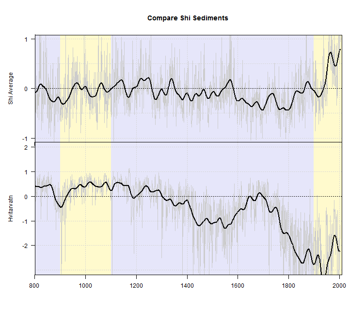
Figure 1. Top – average of five Shi et al varve thickness series; bottom – Hvitarvatn varve thickness (inverted). All in SD Units.
There is no “common signal” in the Kaufman Five according to common methods. The median inter-series correlation is 0.00605, with negative interseries correlation as common as positive interseries correlation. If one examines the eigenvalues of the correlation matrix – a useful precaution in assessing whether the data contains a “common signal” – there are no eigenvalues that are separable from red noise as evident in the barplot below.
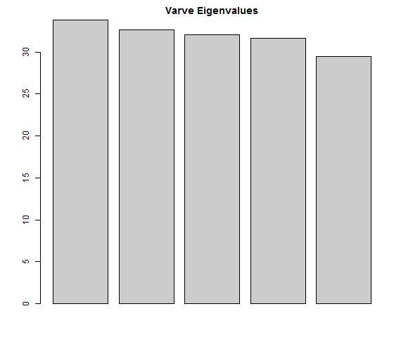
Figure 2. Eigenvalues of (Kaufman Five) Varve Thickness Series
Despite the overwhelming lack of common signal according to these criteria, the average of the Kaufman Five has a distinctly elevated 20th century. Here is a plot of the Kaufman Five. The lack of correlation and lack of significant eigenvalues is evident in the plot, where there is little in common among the series except for one feature: the 20th century in each series is somewhat elevated relative to the 19th century. (As noted above, the average of the five series has a somewhat elevated 20th century, but is relatively featureless in centuries prior to the 20th century, especially in comparison to the well-dated Hvitarvatn series.)
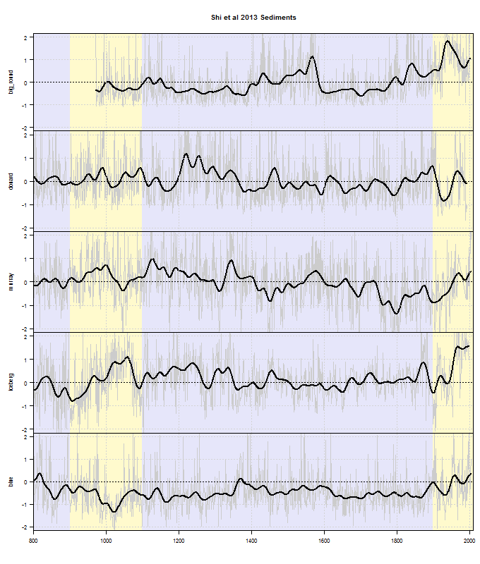
Figure 3. Five Varve thickness series used in Shi et al 2013 (SD Units.)
When parsed in detail, each of the Kaufman Five has troubling defects, some of which I’ll briefly discuss today and which I’ll try to follow up on.
The Iceberg Lake, Alaska series has profound inhomogeneities, especially in its 20th century portion. A major inhomogeneity is that varve thickness is related to distance to the inlet, an observation first made in comments at Climate Audit in comments on Loso 2006. Loso 2009 conceded this point (without mentioning Climate AUdit though it did acknowledge WIllis Eschenbach who corresponded with Loso on a different point) but its remedy (taking logarithms) was hopelessly inadequate to the problem. Dietrich and Loso 2012 acknowledges that inhomogeneities impact their reconstruction, but did not amend or withdraw the earlier series. Interestingly, Dietrich and Loso report glacier advance in Alaska commencing around 1250AD, almost exactly contemporaneous with the well-dated Hvitarvatn advance. The Iceberg Lake series, as used, has a late 20th century uptick coinciding with a major inhomogeneity, the effect of which cannot be separated under any plausible technique known to me.
Major features of the Big Round Lake series (as I’ve observed previously) correspond to major features of the Hvitarvatn series and there is a much higher inter-series correlation between these two series than to other series in the Kaufman Five. The only problem is that this correlation requires inversion of the Big Round series so that thicker varves are generated in the Little Ice Age. There are important geological parallels between the two sites: like Hvitarvatn, Big Round is a proglacial lake, the sediment volume of which is related to proximity of a nearby glacier, which advanced in the Little Ice Age to its Holocene maximum and receded in the 20th century. In order to use the Big Round series in its present orientation, specialists have to explain why its behavior is opposite to Hvitarvatn. And why one should interpret Big Round varve data as showing a Little Warm Period in Baffin Island during Iceland’s Little Ice Age (especially when glacier lines moved 500 m lower in Baffin Island during this period.) The reason why Big Round varves are oriented thick-up by the original authors (Thomas et al 2009) is that there is a positive correlation in the late 20th century between varve thickness and local temperatures. Together with the exclusion of the inhomogeneous Iceberg Lake series, inverting this series (as seems required) would obviously impact the average of the canonical series.
Like Hvitarvatn and Big Round Lake, Donard Lake (Baffin Island) is a proglacial lake whose sediment volume is controlled by proximity of a nearby glacier (Caribou Glacier). Once again, this glacier reached its Holocene maximum in the Little Ice Age, prior to its 20th century retreat. However, the Donard Lake varve thickness series has a slightly negative correlation to the Big Round Lake series. Rather than simply averaging these two incompatible series, specialists need to closely re-examine the data to explain the inconsistency. Donard Lake dating is one thing that needs close examination.
Thomas and associates have recently reported a third proglacial varve thickness from Baffin Island (Ayr Lake), for which they unable to report a significant correlation to instrumental temperature. Thus, they did not report a temperature reconstruction for this site. However, the absence of such correlation surely bleeds back to the other series, inviting a reconsideration of whether their supposed correlations to temperature were spurious – particularly in the context of their inconsistency with the well-dated Hvitarvatn series.
Because varve thickness in these proglacial lakes is profoundly affected by glacier proximity, there is no homogeneous relationship between varve thickness and temperature


37 Comments
Is there not a need for a prior step on data such as the Kaufman 5?
That step would be determination of whether there is any useful signal among the noise.
In exploration geochemistry in my time, the data shown here would probably not have been accepted as a on which to build a complex set of statistics and inferences.
An interesting and particularly well documented Norwegian study here from glacial lake sediments in northern Norway, above the Arctic circle- The study is unfortunately in Norwegian, but the abstract and figures are in English. It clearly shows the impact of the LIA.
Link: https://bora.uib.no/bitstream/handle/1956/6068/97160206.pdf?sequence=1
¨
Abstract:
Svartfjelljøkelen is a small (5 km2), maritime ice cap situated on a mountain plateau on the Bergsfjord peninsula in Finnmark, Northern Norway, with an average equilibrium line altitude (ELA) close to 870 m altitude. Several prominent moraines are deposited between the present day glacier snout and the downstream lake Bergsfjordvatnet. Photographs show that the glacier has receded substantially during the last 100 years or so. In an effort to reconstruct continuous glacier activity throughout the Holocene (<11 700 year), two piston cores and HTH-cores were retrieved from the downstream lake, which annually receives sediment laden melt water originating from the glacier, for further analysis. The lake was mapped using ground penetrating radar (GPR) prior to coring in order to secure that analysis were carried out on cores that are representative of the general influx of sediments. The lake sediments were analysed by investigating geochemical elements (XRF), rock magnetic properties, dry bulk density (DBD), weight loss-on-ignition (LOI) and grain size distribution. The resolution of the various methods range from 5 cm to 0,005 cm. Sediment samples were collected from the surrounding catchment in order to cross-validate the glacier signal, as observed in the lake. The relationship between MS and titanium proved, together with the MS versus manganese/titanium, to be particular good indicators of glacial and extra-glacial sediment sources. 210Pb dating of the uppermost sediments and 14C dating of macrofossils throughout the piston cores provided a robust age-depth relationship that covers the last 9000 years. Quaternary geological mapping of the area revealed the impact of glaciofluvial, fluvial and colluvial processes. Marginal moraines were indirectly dated using historical records, which again were connected to certain levels in the lake sediments. This was feasible due to successful 210Pb dating of the lake sediments. By tying the age of the moraines to the independently dated lake sediments, a regression was constructed that allows for a continuous ELA reconstruction. This reconstruction was used, by means of the Liestøl equation, to calculate variations in winter precipitation for the corresponding time interval. Here it is demonstrated that Svartfjelljøkelen retreated between 9000 and 7000 cal. yr BP, with a brief glacier advance around 8200 years ago. There was arguably little or no glacial input in Bergsfjordvatnet between 7000 and 5200 cal. years BP. After this the glacier advanced throughout the “Neoglacial”, until Svartfjelljøkelen reached its maximum extent during the “Little Ice Age”. This overall trend is coherent compared to other glacier reconstructions from Northern Norway, however variations on multi-decadal time scales are observed that possibly reflect more local climatic changes and/or uncertainties associated with the methods employed in this study.
I looked up the Wikipedia article on varves (because I didn’t know exactly what they were) and found an interesting quotation: “By 1914, De Geer had discovered that it was possible to compare varve sequences across long distances by matching variations in varve thickness, and distinct marker laminae. However, this discovery led De Geer and many of his co-workers into making incorrect correlations, which they called ‘teleconnections’, between continents, a process criticised by other varve pioneers like Ernst Antevs.” [bold mine]
When I learnt Quaternary Geology back in the seventies “teleconnections” were considered a classical case of a failed technique based on wishful thinking.
Plus ca change, plus c’est la même chose.
Notice that they have to excuse themselves and put the mandatory brackets around “The Little Ice Age” and make mandatory consessions to the “consensus”b view that the LIA was local and/or an artifact of shortcomings of the Methods employed in the study.
Who said climate scientists are not humble?
Interestingly there are no brackets around ‘den lille istid’ (LIA) in the Norwegian text, but then I don’t think anyone has seriously tried to dispute its existence in Scandinavia.
I appreciate both articles. It was an easy read for a layman, and helps in my understanding.
I would have expected the eigenvalues to show some signal! Hmm.
Steve wrote:
“Because varve thickness in these proglacial lakes is profoundly affected by glacier proximity, there is no homogeneous relationship between varve thickness and temperature”
These topics predate AGW, of course. This (still paywalled!) paper addresses some of the questions raised in the comments:
“Correlation of Alaskan varve thickness with climatic parameters, and use in paleoclimatic reconstruction” James A. Perkins and John D. Sims, 1983
Abstract
The thickness of varves in the sediments of Skilak Lake, Alaska, are correlated with the mean annual temperature (r = 0.574), inversely correlated with the mean annual cumulative snowfall (r = −0.794), and not correlated with the mean annual precipitation (r = 0.202) of the southern Alaska climatological division for the years 1907–1934 A.D. Varve thickness in Skilak Lake is sensitive to annual temperature and snowfall because Skilak Glacier, the dominant source of sediment for Skilak Lake, is sensitive to these climatic parameters. Trends of varve thickness are well correlated with trends of mean annual cumulative snowfall (r* = .902) of the southern Alaska climatological division and with trends of mean annual temperature of the southern (r* = .831) and northern (r* = .786) Alaska climatological divisions. Trends of varve thickness also correlate with trends of annual temperature in Seattle and North Head, Washington (r* = .632 and .850, respectively). Comparisons of trends of varve thickness with trends of annual temperature in California, Oregon, and Washington suggest no widespread regional correlation. Trends of annual snowfall in the southern Alaska climatological division and trends of annual temperature in the southern and northern Alaska climatological divisions are reconstructed for the years 1700–1906 A.D. Climatic reconstructions on the basis of varve thickness in Skilak Lake utilize equations derived from the regression of series of smoothed climatological data on series of smoothed varve thickness. Reconstruction of trends of mean annual cunulative snowfall in the southern Alaska climatological division suggests that snowfall during the 1700s and 1800s was much greater than that during the early and mid-1900s. The periods 1770–1790 and 1890–1906 show marked decreases in the mean annual snowfall. Reconstructed trends of the annual temperature of the northern and southern Alaska climatological divisions suggest that annual temperatures during the 1700s and 1800s were lower than those of the early and mid-1900s. Two periods of relatively high annual temperatures coincide with the periods of low annual snowfall thus determined.
[I have inserted “r*” where the paper had “r” with an overscore, not sure how to reproduce the overscore in my browser – Matt]
So it was well known 30 years ago that snowfall confounds temperature in proglacial lake sediment varve thickness. On the west coast of the US, snowfall occurs when marine moisture meets cold, dry arctic air. This is weather more than it is climate. Note that the coldest periods, 1770–1790 and 1890–1906, somewhat coincide with the coldest periods in the other proglacial lakes. I would surmise that the cessation of snow during these periods would be related to the weather we have right now, a massive dome of frigid arctic air keeping marine systems well off the coast.
“Comparisons of trends of varve thickness with trends of annual temperature in California, Oregon, and Washington suggest no widespread regional correlation.” What does this say about reconstructions which estimate global or hemispherical temperature history from widely scattered proxies? Even if the proxies were ideal thermometers for the meteorological vicinity, they are not necessarily representative of the region. Yet the reconstruction methodology posits that they are.
Is not this analysis merely a round-about way of pointing to the flaw in the basic approach to almost all of these temperature reconstructions, i.e. selection of proxies based on the correlation of the response to the instrumental record (as it very clearly is noted in the Shi et al 2013 paper)? Do not these authors of temperature reconstructions realize how easy it is to obtain a low frequency correlation between an upward trending observed temperature and any other upward trending measurement – and without a direct cause and effect relationship between the two variables.
That there is poor correlation between these proxy responses is evidently not a major concern with these authors as the stated criteria does not include that relationship. The authors might attempt to wave away these concerns by noting that there are regional differences in temperatures, which there well may be, but as SteveM has been careful to note the discrepancies between proxy responses are over extended periods of time. Unfortunately if temperatures were spatially varying in this manner (over extended periods of time) the uncertainty of any estimated mean regional temperature that encompasses these locations should have properly calculated confidence intervals from the floor to the ceiling.
I continue to attempt to rationalize the conceptual blind spot that allows these authors to continue to make this basic error in their approach to temperature reconstructions. Perhaps part of it is that in their hurry to confirm their prior beliefs that we are in an “unprecedented” warming they see a correlation in some proxy responses in the same upward direction as temperature and proceed to stop thinking and start publishing.
Steve: the older specialist literature on varves shows very clear understanding that varve thickness is not linearly and homogeneously related to current temperature, but seem to be ignored in the articles proposing these various temperature reconstructions from varves.
Well, that was supposed to be fixed by the shiny new methodology used by Gergis-Karoly-Neukom. Filter out the low-frequency signal and select proxies by using the high-frequency signal only. And we know how that worked out.
“Well, that was supposed to be fixed by the shiny new methodology used by Gergis-Karoly-Neukom. Filter out the low-frequency signal and select proxies by using the high-frequency signal only. And we know how that worked out.”
It can easily be shown that two series with very good correlation (higher frequency correlation) can have very different trends (low frequency correlation). Ideally one would want a proxy response that shows both good high and low frequency correlations with the observed temperature – like a thermometer does. The conundrum is that temperature reconstructions are carried out primarily to look at low frequency phenomena (trends) which would point to finding temperature responses of proxies to temperature trends. The problem there is that finding a spurious low frequency correlation between two trending variables is not difficult at all and particularly when you are selecting proxies.
I believe it is the dendroclimatologist, Rob Wilson, who has always reminded us of the consistency of tree rings to record prominent historical volcanic events, i.e. a potential proxy getting a high frequency response correct. The problem remains that those responses, even in close proximity, do not have nearly the same magnitude in response and it is that near same magnitude in a proxy response that would be required to properly proxy a temperature trend.
E.M. Leonard studied varve chronology at Hector Lake, ALberta and observed that high sedimentation rates occurred during periods of moraine deposition (ice maximums) or during rapid recession (this certainly seems consistent with the Hvitarvatn data.
The temperature reconstruction jockeys seem to have lost contact with previous scientific knowledge about varves. A number of the early temperature reconstructions using varves were from Raymond Bradley’s students :(.
this is off topic, but Dr. Leonard was a professor of mine in college. He had a comic on his office door that depicted some arctic explorers looking at their dog sled. All of the harnesses were empty and laying on the ground. The caption was, “Well, that’s it. We’ve eaten the last of the geologists.” This was 30 years ago. Seems like things haven’t changed that much.
So the proxy actually has a “U”-shaped response to ice extent. This reminds of the work trying to compensate for age in tree rings, which is also “U”-shaped except the “U” is inverted. Somebody – was it Craig Loehle? – showed that with a “U” shaped response to an independent variable buried in the data, the correlation to the variable of interest was always going to be indeterminate no matter how fancy your math. Jim Bouldin’s excellent series of blog posts on treemometry using synthetic data supported similar conclusions. Since ice extent at any given time correlates poorly to temperature at that same time, the same limitations seem to apply.
Kenneth,
Are you saying that much of what we see is noise? That’s how it looks to me. I agree with Steve’s comments about using simple algebra as an aid to rejection of low quality data, and I agree – as would most of us, I guess – that the desirable path of data evaluation is from high quality down. But then, my experience might be atypical because in mineral exploration we were most interested in the fine structure of anomalous values, whereas the dominant trend in climate work is to reject or smooth them. Rejection of the anomaly (in its broad definition, not the climate one) is possibly approaching the data from the wrong end.
if you view unexplained variance as noise, its easy to go down that road. Instead of looking at the data available and thinking that we don’t really know how to explain what we all can see, we smooth away anything we think is noise. The urge to draw conclusions from momentary glimpses at the underlying physics must be strong indeed… unless its the late 20th century…in that case, the variance isnt noise, its signal. give me a break.
“Are you saying that much of what we see is noise?”
Those doing the reconstructions admit to that. Unfortunately their approach cannot extract a signal because selection of proxies after the fact does not allow for “subtracting out” noise – assuming that the noise is random. There may well be valid temperature proxies out there but those doing the reconstructions are so wrongheaded in approach and unwilling to do the preliminary work that finding and differentiating those proxies from the invalid ones will not be an easy task.
I suspect the field you worked in was driven by profit and loss and involved science that was “harder” than that used in constructing temperature proxies. You had the opportunity to conclusively test the validity of your methods – and without waiting years for out-of-sample test results. And profit and loss are good motivators for getting it right or at least better.
Steve, you stated that:
“the older specialist literature on varves shows very clear understanding that varve thickness is not linearly and homogeneously related to current temperature, but seem to be ignored in the articles proposing these various temperature reconstructions from varves”
When did the transition between it being generally believed that varves were poor temperature proxies to being generally accepted that they were a valid means of determining regional temperature?
Interesting question that I’ve been wondering about. It looks like Raymond Bradley and his students had a large hand in it. Lamoureux and Bradley 1996 did a temperature reconstruction for Lake C2 on Ellesmere Island. They considered the possibility of inhomogeneity but set it aside. Once a couple of reconstructions were in print, they seem to have been relied on as authority without the contradicting literature being cited.
Their introduction into multiproxy studies seems to be mostly due to Kaufman et al 2009.
I don’t think that any of the TAR multiproxy reconstructions (including MBH) used any. Bradley, Hughes and Diaz 2003 used a couple of varve series (Murray Lake and one other). Kaufman used all of the varve series that are now “canonical”. Following Kaufman, they became widely used – in the various Ljungqvist studies, PAGES2K, Shi. However, the repertoire of varve thickness series becomes fairly stereotyped.
In my ongoing naïveté I would expect a broad series of major, rigorous calibration and validation studies of diverse locales and conditions before any scientist would even begin to treat varves as reliable temperature proxies.
What kind of scientific field treats casual guesswork as confirmed scientific results??
Looking more closely, Overpeck et al 1997 used six lake series, including C2 and Donard.
After reading the varve posts, my concept of their validity as a temperature proxy has become consdierably muddier.
LOL!
Bottom Feeders?
So:
1. Find paleo series which are proxy to multiple physical phenomena among which conceivably temperature.
2. Data mine for a hockey stick from any of the phenomena.
3. Claim temperature as THE phenomena causing the hockey stick.
Next week we’ll cover climate science communications. Read up.
==================
aahhhh, Kim, surely there is a more sympathetic way to describe such sophisticated, rigorous, and “bullet-proof” scientific procedures….
p.s. I do enjoy how you can describe the methods of current ClimateScience-TM so succinctly.
I wonder if you have a stratospheric overview of temperature reconstructions of the past. What are all the methods used, what are the problems (and strengths) of each of them, and which (if any) do you consider reliable?
Steve McIntyre Posted Dec 5, 2013 at 6:29 PM
This was the subject of my discussion with Michael Loso, and the question to which he never replied. I came across the reversal when I took a look at how the Iceberg Lake varve thickness compared to the local temperature. There was a good fit … except it was 180° out from what Loso claimed. He was saying that the thick varves were a sign that it was warmer weather than usual … but the data showed that thick varves were correlated with cold weather.
He never answered this, presumably because he’d have to retract a bunch of his previous assertions … the details of all of this were published and discussed on CA back in 2007, the graphs are here.
w.
Although I am a geochemist and a geologist only by contamination, it can be noted that sedimentary deposition is a major topic in geology. In some places it has special features that draw specialist studies. One such case is the Brockman Iron Formation in West Australia. There are hundreds of references to past work, an entry level one being http://ammin.geoscienceworld.org/content/90/10/1473.short
“…..microbanding is especially well developed in the Brockman Iron Formation of Western Australia, where it has been interpreted as chemical varves, or annual layers of sedimentation. BIFs ranging in age from 2.2 Ga to about 1.8 Ga…”
These BIFs are among the types of iron ores mined on a large scale and that has attracted extra study focus. Despite the study and the observation of pattern matching of fine banding over distances of hundreds of km, there are many remaining unknowns about the factors affecting deposition. The science is not settled. The cited article uses cautious prose as if more developments are expected.
Unless one is a specialist in sedimentary geology, perhaps even a specialist in geological pattern matching, it is naïve to make correlations between patterns and depositional history within modern sediments. One might say that we can observe the present conditions of deposition to our advantage and hence infer more than we can from old rocks, which is in part correct. The other part is that some parameters can change in the time between the deposition we observe today and those that are eventually recorded when the sediments are lithified to a long-term constancy. That is why geos have terms like penecontemporaneous dedolomitization, to use Nth American spelling.
One short message is that you cannot write a definitive paper when you do not know (and cannot know) some past conditions. The known and unknown unknowns appear to exert too large an influence to allow definitive statements. That is what I meant above when suggesting that one has first to establish that a useful signal can be separated from the noise. The ‘noise’ here is the unknowns, which can show themselves in data that goes up at one place and time and down at a nearby place at a similar time – as Steve has illustrated with the 5 graphs of Shi sediments. (To average these, if that was done, is schoolboy howler stuff).
Another short message is that you cannot swoop in wearing a ‘climate scientist’ seal of approval and expect to be correct.
Surely you could titrate the degree of contamination, Geoff ?
I mean, being a chemist and all … 🙂
Speleothems are used as a proxy for temprature at a given age. Why can’t plain limestone be used for the same purpose?
As a specialist in sedimentary geology (aka sedimentologist), I was tempted by your comment to dip into my copy of Reading (ed) Sedimentary Environments. There is a chapter on lakes, as well as a section on glaciolacustrine environments. Lakes are completely outside my area of expertise.
Paraphrasing glaciolacustrine environments.
Glacier-fed lakes are divided into ice-contact lakes and distal (non-contact) lakes fed by outwash streams. The main factors that affect physical processes and sedimentation are proximity to the ice, thermal stratification of lake water, and seasonality of inflowing meltwater and ice cover. Thermal stratification is inhibited by ice contact. Contact/non-contact may evolve with time. Stratification leads to autumnal overturning of the water layers and this influences sedimentation patterns.
In lake basinal sub-environments, seasonal fluctuations are recorded as rhythmites and varves. Sediment is deposited from suspension and by density currents, turbidity currents and mass flow. A typical succession contains rhythmically laminated or varved fine sand to clay interrupted by turbidites, current rippled sand deposited by bottom-hugging flows, and massive or graded diamicton beds deposited by mass flows.
Moving on to lakes (rhythmites).
Lamination style depends on stratification regime and suspended sediment supply. Lakes may be stratified, unstratified or partly stratified and partly unstratified. Suspended sediment supply may be continuous, discontinuous, discontinuous during stratification, discontinuous during non-stratification or discontinuous during stratification and non-stratification.
I would suggest, as is the case with statisticians, this is an area that would benefit from the employment of specialists. Limnologists, for example.
Thanks for the link Geoff, I enjoyed reading that. I’ve spent a lot of time doing fieldwork in the Mt Brockman area. I will take issue with this:
BIFs of the Hamersley Range were deposited on continental crust, and according to my knowledge of plate tectonics, continental crust doesn’t floor deep ocean basins. I have also identified to my satisfaction, plenty of ripples and large scale cross-bedding structures in BIFs. These indicate the influence of waves as well as significant currents on BIF sediments. Sedimentary structures apart from lamination may not be described in the literature, but that doesn’t mean they aren’t there. I suspect that most of the descriptive work has been done by hard-rockers who weren’t looking for and weren’t qualified to recognise them.
Also, the BIF literature is completely wrong in another area. The standard evolution goes: deposition -> compaction -> lithification -> deformation. In fact, some BIFs are full of soft sediment deformation structures (boudinage) and their aspect ratios indicate minimal compaction. A more correct evolution is: deposition -> deformation -> lithification. Compaction and D1 go straight out of the window. Not to criticise hard-rockers, but they shouldn’t stray into areas outside their competence. That’s why I stay away from maths and stats.
Hector,
I was not endorsing a deposition mechanism, merely quoting some papers that might lead into further relevant reading. The main point is that there remains a good deal of scientific uncertainty in sedimentology; and while interpretative uncertainty exists, it is not safe to do some types of statistics because you do not necessarily know which variables need to be quantified and included.
Our team was strong on colloidal phases in sedimentary rock formation – I have not seen a mention of this possible mechanism in the papers referred to above, so that might serve as an example of ignoring a variable or a process that might?? be part of the required analysis.
Thanks Geoff. I didn’t mean to imply you were endorsing anything, simply making a more general point that it’s easy to fall into traps.
I know for certain that anyone who qualifed with a geology degree in Western Australia between about 1975 and 1995, could have done so without ever seeing any sedimentary rocks, either in the field or in hand specimen. If said geo was working with a mental model “laminated sediments = low energy environment”, then they may not have been looking for sedimentary structures. As the mineralogy is massive chert +- Fe, these features may be quite subtle.
I’m intrigued by your reference to colloidal phases. There can be no doubt that these chemical sediments behave as particles, otherwise they would not develop cross bedding. Perhaps I should consult a geochemist. I’ll bring my long handled spoon when I go to sup.