Last year, a paper of mine (Lewis 2014) showing that the approach used in Frame et al (2005), which argued for using a uniform prior for estimating equilibrium (strictly, effective) climate sensitivity (ECS), in fact led to a unique, objective Bayesian estimate for ECS upon undertaking a simple transformation (change) of variables. The estimate was lower, and far better constrained at the upper end, than the one resulting from use of a uniform prior in ECS, as recommended in Frame et al (2005) when estimating ECS. The only uniform priors involved were those for estimating posterior probability density functions (PDFs) for observational variables with Gaussian (normally distributed) data uncertainties, where they are totally noninformative and their use is uncontroversial. I wrote an article about Lewis (2014) at the time, and a version of the paper is available here.
I’ve now had a new paper that uses an essentially identical method to Lewis (2014), but with updated, higher quality data, published by Climate Dynamics, here. A copy of the accepted version is available on my web page, here.
Like many climate sensitivity studies, the method involves comparing observationally-based and model-simulated temperature data at many differing settings of model parameters, a simple global energy balance model (EBM) with a diffusive ocean being used. But, unusually, surface temperature observational data were not used directly. Like Lewis (2014), my new paper uses observationally-constrained estimates of global mean warming attributable purely to greenhouse gases, separated using detection and attribution methods from temperature changes with other causes, treating them as “observable” data. Effective heat capacity, the ratio of ocean etc. heat uptake to the change in global mean surface temperature (GMST), is used as a second observable. It is estimated using the AR5 planetary heat uptake estimates spanning 1958–2011 and HadCRUT4v2 GMST data.
Detection and attribution studies involve coupled 3D global climate model (GCM) simulation runs with different categories of forcing. They use multiple-regression techniques to estimate what scaling factors to apply to the GCM-simulated spatiotemporal temperature response patterns for the various categories of forcing in order to best match their sum with observational data. The scaling factors (being the regression coefficients) adjust for the GCM(s) under- or over-estimating the responses to the various categories of forcing and/or the forcing strengths. So the estimates of GHG-attributable warming they produce, used as input data in my study, are fully constrained by gridded observational temperature records. This approach is potentially better able to isolate aerosol forcing, the biggest cause of uncertainty when estimating ECS from warming over the instrumental period, than methods using low dimensional models. I used estimates from the same multimodel detection and attribution studies that underlay the main anthropogenic attribution statements in the IPCC fifth assessment Working Group 1 report (AR5), Gillett et al (2013) (open access) and Jones et al (2013), based on their longest analysis periods (respectively 1861-2010 and 1901-2010).
The abstract from my paper reads as follows:
Equilibrium Climate Sensitivity (ECS) is inferred from estimates of instrumental-period warming attributable solely to greenhouse gases (AW), as derived in two recent multi-model Detection and Attribution (D&A) studies that apply optimal fingerprint methods with high spatial resolution to 3D global climate model simulations. This approach minimises the key uncertainty regarding aerosol forcing without relying on low-dimensional models. The “observed” AW distributions from the D&A studies together with an observationally-based estimate of effective planetary heat capacity (EHC) are applied as observational constraints in (AW, EHC) space. By varying two key parameters – ECS and effective ocean diffusivity – in an energy balance model forced solely by greenhouse gases, an invertible map from the bivariate model parameter space to (AW, EHC) space is generated. Inversion of the constrained (AW, EHC) space through a transformation of variables allows unique recovery of the observationally-constrained joint distribution for the two model parameters, from which the marginal distribution of ECS can readily be derived. The method is extended to provide estimated distributions for Transient Climate Response (TCR). The AW distributions from the two D&A studies produce almost identical results. Combining the two sets of results provides best estimates [5–95% ranges] of 1.66 [0.7 – 3.2] K for ECS and 1.37 [0.65 – 2.2] K for TCR, in line with those from several recent studies based on observed warming from all causes but with tighter uncertainty ranges than for some of those studies. Almost identical results are obtained from application of an alternative profile likelihood statistical methodology.
The posterior probability density functions (PDFs) for the two ECS estimates are shown in Figure 1. The exact match of best estimates and uncertainty bounds using the alternative frequentist profile likelihood method confirms that the objective Bayesian method used provides frequentist probability-matching.
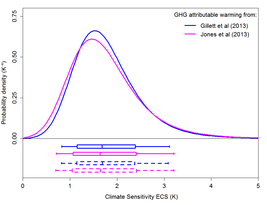 Figure 1. The box plots indicate boundaries, to the nearest grid value, for the percentiles 5–95 (vertical bar at ends), 17-83 (box-ends), and 50 (vertical bar in box), and allow for off-graph probability lying between S = 5 K and S = 20 K. Solid line box plots reflect the percentile points of the CDF corresponding to the plotted PDF. Dashed line box plots give confidence intervals derived using the SRLR profile likelihood method (the vertical bar in the box showing the likelihood profile peak).
The revised best (median) estimate for ECS in Lewis (2014) using the objective Bayesian approach, after correcting data handling errors, was 2.2°C. It seems likely that estimate was biased high by the use of temperature data spanning just the 20th century, which started with two anomalously cool decades.
The new study’s best estimate for ECS is almost identical to that of 1.64°C obtained in Lewis and Curry (2014). That study used a simple single-equation energy budget model to compare, between periods spanning 1859–2011, the rise in GMST with forcing and heat uptake estimates given in AR5. As it relied on the expert assessment of aerosol forcing given in AR5, which spans a very wide range, the ECS estimate upper uncertainty bound was higher, at 4.05°C, than in my new study.
The ECS estimate in my new study is also very similar to that in Lewis (2013). That study compared the evolution of surface temperatures in four latitude zones with simulations spanning 1860– 2001 by the MIT 2D global climate model (GCM). Many simulations were performed with differing parameter settings and hence varying model values of equilibrium/effective climate sensitivity (ECS), ocean effective vertical diffusivity (Kv) and aerosol forcing – which can be tightly constrained when zonal rather than GMST data is used. The parameter combination that best fitted the observational data gave a median estimate for ECS of 1.64°C. With non-aerosol forcing etc. uncertainties adequately allowed for, the 5–95% uncertainty range was 1.0–3.0°C.
Figure 2 shows posterior PDFs for the two TCR estimates from my new study. The best estimates are within 0.05°C of each other. Their average is 1.37°C, with a 5–95% range of 0.65–2.2°C. This is within a few percent of the best estimates for TCR in Lewis and Curry (2014), and of those given in Otto et al (2013), of which I was a co-author alongside fourteen AR5 lead authors.
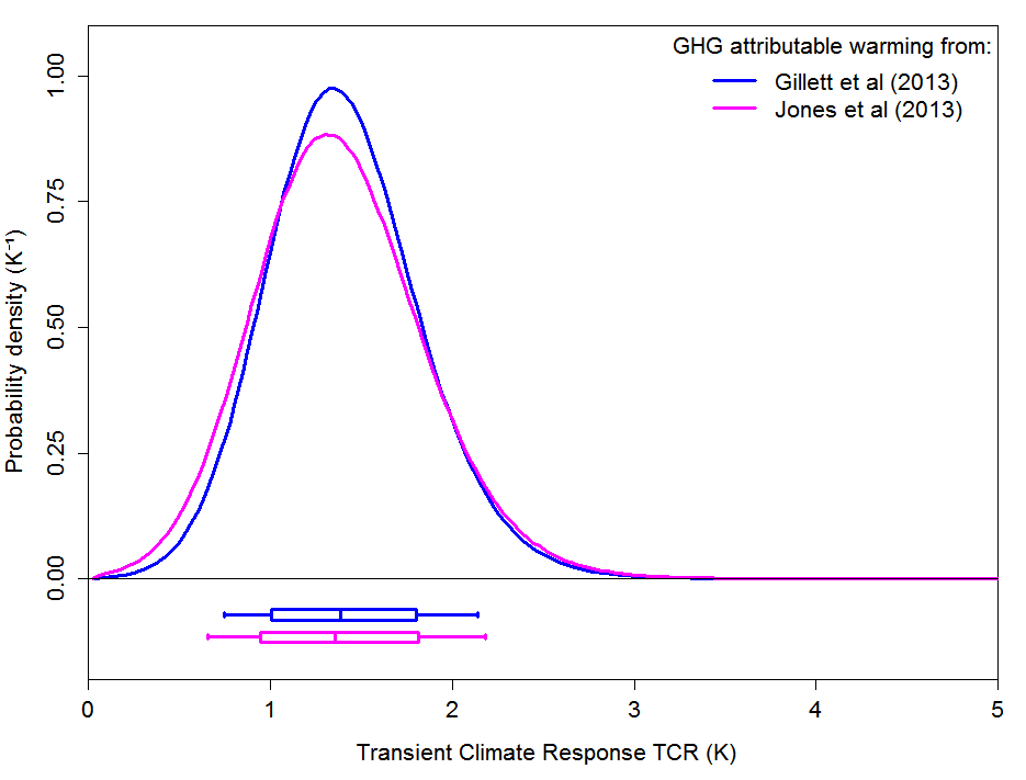 FIG. 2: Estimated marginal PDFs for transient climate response derived, upon integrating out Kv, using the transformation of variables method. The box plots indicate boundaries, to the nearest grid value, for the percentiles 5–95 (vertical bar at ends), 17-83 (box-ends), and 50 (vertical bar in box). They reflect the percentile points of the CDF corresponding to the plotted PDF.


141 Comments
The Bishop Hill blog had a posting containing tweets from a conference at which Myles Allen presented. Allen was reported to have strongly criticized the Otto paper with the correspondent commenting that he was surprised that Allen was so critical of a paper of which his was a co-author. Does Nic Lewis have any comments on Allen’s objections to the Otto paper’s results?
Relevant tweet about Allen’s description of Otto paper is:
I don’t know the grounds for Myles Allen’s objections or even to what exactly he objected, so I can’t comment, I’m afraid. He didn’t voice any objections to Otto et al (2013) in his talk at the March 2015 Ringberg climate sensitivity workshop at which we were both participants, as far as I recall. I’ve no idea what “ignores the disequilibrium effect” refers to.
I don’t see any reason for strong criticism of the Otto et al energy budget study, although I think the Lewis and Curry (2014) study preferable.
Nic,
The most common critique of all EBM based estimates of equilibrium climate sensitivity is the Armour et al, Journal of Climate (2013) argument of large differences in regional response rate, with the highest sensitivity regions, at higher latitudes, being much slower to respond than the rest, leading to incorrect (low) estimates based on the ‘early’ response to forcing (that is, discounting any EBM equilibrium sensitivity estimate that is based on the instrument temperature record). Of course, the CMIP models do not all agree with Armour et al, but many do shot substantial temporal non-linearity in response. Does your 2013 paper (with 4 modeled latitudinal regions) offer anything to refute the Armour et al argument? Seems to me the same argument would not apply to EBM based estimates of transient response.
Steve,
I think Kyle Armour’s single-model analysis has been rather superceded by multimodel analyses, in particular Andrews, Gregory and Webb (2015): The dependence of radiative forcing and feedback on evolving patterns of surface temperature change in climate models. They find that the majority of the reduction in the global climate feedback parameter over time comes from the tropics, not high latitudes. The highest sensitivity regions in many models are in the deep tropics, not high latitudes.
The shortfall in effective climate sensitivity (as one would expect energy budgets to estimate) from the usual 150 year Gregory plot estimation of model ECS values (as given in AR5) is quite modest for the CMIP5 mean.
My 2013 paper estimates effective climate sensitivity but with a value calibrated to the equilibrium sensitivity of the (2D MIT) GCM involved. I am unsure how the time variation of climate feedback strength in that model compares with other models.
I don’t think time varaition of feedback strength has any implications for TCR estimation, and (for the average model) it makes a pretty negligible difference in warming over the first 200-300 years.
This battle will not be over until climate scientists accept the fact that the lower bound of CO2 warming is negative and the overall result of adding CO2 to an atmospheric mix can include cooling as an outcome.
Depends which battle. This could be seen as slayers vs delayers – those like myself who feel that attempts to cut carbon emissions have gone too far (or at least too stupid) too fast. The sensitivity bounds Nic finds by constraining to real world data sit well with delaying – and finding out far more with the passage of years – without any need to pronounce a negative lower bound.
Just out of curiosity – how do you compensate for missing coverage in the surface temperature record. From what I can see you only use HadCRUTv2 and make no allotment for coverage bias (which is undoubtedly real and makes a difference).
Using BEST or CW2014 gives temperature change values of ~0.56°C and ~0.58°C on the same time periods as you use which is an appreciable difference from the 0.52°C result you use. Using a later period (e.g. 2004-2014) gives ~0.57°C and 0.59°C, respectively.
At some point you’re going to have to explain your rationale for assuming that the unsampled portions of the Earth are changing at the same rate as the global average (e.g. HadCRUTv2). There is very strong evidence that this is not the case from satellites, remote weather stations, atmospheric reanalysis and physical phenonenon. These nuances in the research are important and if you have concerns with these datasets then you should publish your concerns or be willing to respond and read the evidence which contradicts those views.
Robert if its possible can you say ( back of the envelope ) what difference you think those numbers would make to the ECS and TCR?
I believe when Robert asked last time RE the sensitivity of the estimates to using the BEST or CW products that Nic’s response was essentially “not sensitive”.
seeing the actual numbers run would put this issue to bed.
I remain perplexed why that is so hard
Robert,
If you think there is an additional 10% warming that is not accounted for in HADCRUT4, then I guess the best estimate would increase by ~10% (~1.83C per doubling). Is that what you are suggesting, or something else?
Robert,
I’ve explained before in response to near identical comments from you why I make no adjustments to the HadCRUT4 datasets. Doing so does not imply that I think unsampled areas all warm at the same rate as the global average.
Anyway, in this case your comment shows that you have not understood my study. Increasing the HadCRUT4v2 0.52 K increase in GMST between means for 1958-68 and 2001-11 to the CW2014 estimate of 0.57 K would REDUCE my study’s best estimate of ECS by about 2%, not increase it!
It is the choice of surface temperature dataset made by Gillett and Jones for their attribution studies that I would expect you to be more concerned with, as my ECS estimates scale with their increases. Both chose HadCRUT4v2. I don’t expect you’ve calculated the difference between the HadCRUT4v2 and CW2014 warming trends over 1901-2010, the analysis period used in Jones et al 2013. They are actually the same, both being 0.075 K/decade. For Gillett et al 2103, over its 1861-2010 analysis period CW2014 warms 8% faster than HadCRUT4v2. If you want for your purposes to adjust my ECS estimate by 2% ([0% + 8%]/2 – 2%: including for both the average of 1901-2010 and 1861-2010, and for 1958-68 to 2001-11) then go ahead and do so.
Nic,
How can a greater warming (more warming than HADCRUT4) with everything else the same lead to lower sensitivity estimates? I really don’t understand.
I guess it depends upon when the warming occurs.
The time difference between the two is 1861 to 1901 which means that CW2014 must have more warming in this period than HadCRUT4v2.
More warming before CO2 increases implies less sensitivity to CO2 and more natural variability.
Steve,
If you read the paper it should be clear to you. The warming Robert W referred to is used purely to estimate effective (ocean etc) heat capacity (EHC), being delta_OHC/delta_GMST. A higher GMST value gives a lower EHC estimate, which implies a smaller difference between the multidecadal and the equilibrium warming caused by a given GHG forcing increase.
Dr. Lewis,
This paper relies on some input from modeling studies, which I assume is necessary. I have never seen a sensitivity study that relies entirely on interpretations of empirical data. It seems we have upwards of 15 years of good data and that should be enough to at least make an estimate, albeit with wide error bars. Could you briefly explain the limitations of the empirical data that prevent a sensitivity estimate without model input?
It is impracticable to obtain estimates of effective radiative forcing without use of models: even for GHG forcing, some kind of model (not necessarily a GCM) is needed.
Estimates of the very uncertain aerosol forcing will certainly have to involve some kind of climate model, although it could be a simple hemispherically-resolving one. It is very difficult to well estimate aerosol forcing from first principles and empirical data because indirect (cloud change linked) aerosol forcing is thought to have a logarithmic relationship to cloud condensation nuclei (CCN) concentration and is hence very sensitive to the (very poorly known) natural preindustrial CCN level. But energy budget and similar sensitivity studies are not much, if at all, dependent on how sensitive the climate models used to derive forcing estimates are.
15 years of good recent data is helpful, but a much longer period is needed for changes in GMST and ocean heat content to sufficiently exceed natural internal variability. That means looking to changes starting many decades ago, when data was poorer.
Thanks for the bit about CCN, I have been puzzling over this for awhile, figuring that some clever person would figure out how to discern aerosol forcing by teasing out spectral absorption differences or whatever. Sounds like that is only one piece of the puzzle.
Nick,
“I’ve explained before in response to near identical comments from you why I make no adjustments to the HadCRUT4 datasets. Doing so does not imply that I think unsampled areas all warm at the same rate as the global average.”
You’ve never been able to give a coherent answer to why you do not use an improved approach to estimating global surface temperature changes. Whether this makes material difference to this result or to others is not a rationale for excluding the (now three) datasets out there showing more warming than HadCRUTv4.2 due to coverage issues.
In the past it has made a difference to the results of one of your studies (for instance to Lewis and Curry) and it is very odd that you choose not to test your assumptions under the different datasets. Appealing to prior studies usage of a dataset isn’t exactly a convincing argument since there have been various versions of HadCRUT used in the literature over the past 5 years. I’m not even saying it makes an appreciable change on this analysis – what I’m saying is that it would be skeptical to try analysis using a variety of datasets.
Dear Robert:
i can certainly appreciate your concerns regarding Nic’s paper…
One always must be concerned that a time series was picked, not because of its ability to reveal underlying climatic behavior, but rather because its behavior fits into an established paradigm.
Of course, the same could be said for some peoples’ use of contaminated sediment proxies…or for the inclusion of stripped tree bark proxies, some containing a total of 1 (one) tree for periods of time in the time series…the use of varves to infer climatic behavior, when the authors who collected the data, and published the paper from which the data were used, advised against using that data for that purpose. Theres that practice, or lack of practice.
I would suppose that inferring the temperature of the entire antarctic continent from a few stations on the coast wouldn’t be too wise of a practice?
How about using temperature data from the northern hemisphere to infer temperature behavior in the southern hemisphere?
What about inventing a new type of PCA, non centered PCA, a technique which the person who developed PCA felt was indefensible?
I mean really, once one starts to critique the behavior of researchers in this field, when is it reasonable to stop?
I suppose another interested researcher could attempt to independently verify Nic’s result using another temperature time series?
That would be skeptical as well.
You know, email Nic, and ask him for his code, and run the analysis on another data set?
im betting that you won’t get a response along the lines of “Why should i give you my data, youre just going to try to show that I’m wrong”
Anyway, you’ve waded into a pissing contest of historical proportions,. Perhaps because of the scale of grants being awarded for research into this phenomenon?
Nick,
I’m reading through again and I have an issue.
You state in the paper:
“Gillett et al. (2012) found that using data from the twentieth-century, the first two decades of which coincided with an AMO cycle bottom and were anomalously cool, introduced substantial upwards bias into estimation of the GHG scaling factor relative to estimation based on the longer 1851–2010 period.”
Gillett et al. (2012) make no mention of the AMO in that paper and they use an older surface temperature record that does not have compensation for coverage because they’re masked. Currently, warming has been at the upper end of model runs for the Arctic according to Thorne et al (2015) so masking isn’t enough either. If you look out our record for instance you will see the early 1900s were not ‘anomalously cold’.
That you assert that these decades were anomalously cold in the global temperature record (they weren’t relative to the prior decades) and that you believe this was caused by the AMO (a feature we still can’t even isolate the sign of during that period effectively) is incredibly problematic.
Robert,
Gillett et al (2012) says:
“Figure 1a shows that the global mean temperature in the first two decades of the 20th century was anomalously cool”
I didn’t write that Gillett et al 2012 attributed the anomalous coolness to the AMO. I wrote that the first two decades of the 20th century coincided with an AMO cycle bottom. It does, per the widely used NOAA AMO index.
The last two decades of the 19th century were affected by much heavier negative volcanic forcing than the first two or so decades of the 20th century.
Dr Way:
First, I want to thank you for engaging in the discussion this blog. I seek out and read your comments whenever you make them, and I know you’ve been the target of some rather intemperate remarks here, so, thanks again.
In the interest of clarifying areas of disagreement, as well as agreement, in the current debate concerning Equilibrium (or Effective) Climate Sensitivity. I ask the following questions :
1) Why do you think there has been little success in narrowing the uncertainty associated with estimates of ECS over the last thirty years or so?
2) Whats your best guesstimate for ECS?
3) Do you disagree or agree with the proposition that right end of the PDF of ECS estimates produced by scientists and cited by IPCC may be a…bit too long? A bit too wide?
4) If you dont agree with Nic’s choice of a value for his prior, what do you feel would be an appropriate value for the prior used in Nic’s analysis? Any thoughts on how this would affect his calculation for ECS?
5) What do think the appropriate governmental policies should be regarding climate change IF ECS turns out to be in the neighborhood of 1.4-2.0 degrees C?
thanks again.
david
what robert asks is simple.
how robust is the answer to changing temperature datasets.
It would take less time to actually do this and report the number than to debate the issue.
if its 2% then that is actually a bonus point that Nic should actually show. Showing ( not merely claiming) that your result is robust to data selection is something we’ve beat Mann up over. I’m just puzzled at the resistance.
If I understand correctly above, it sounds like Nic has used the more conservative temperature data set with regard to lowering the upper bound of ECS (i.e., he could lower it even more using CW or BEST). This is not the same type of data selection error/bias of which Mann has been accused.
Steven
Your comment should really be addressed to Jones and to Gillett. If they had used different temperature datasets and reported different estimates of GHG-attributable warming, I could have used them. Neither of them did so, and because their analyses are based on gridded data only they could provide an accurate estimate of the sensitivity.
I was able to give an estimate of the sensitivity to the 1958-2011 GMST change used for the EHC estiamte and, if you read my paper, you will see that I did so.
what robert asks is simple.
how robust is the answer to changing temperature datasets.
It would take less time to actually do this and report the number than to debate the issue.
If that’s the case, then go and damn do it, just like you always tell others to do when they ask you questions about best.
“If that’s the case, then go and damn do it, just like you always tell others to do when they ask you questions about best.”
easy when you provide the code.Since I do, I make those comments.
Reading through Nic’s comments it is not clear whether
A) he provides the code.
B) even if he did that might not help, since, it appears the dependency on Hadcrut4 is upstream. That is, he built his results on something we can’t check.
It looks like Nic chose papers that rely on hadcrut4, and that choice means we can’t get the answer to the question in any kind of definitive way. it is what it is.
There is an analog in open source when people build on or inlclude code that is closed. basically that choice infects everything.
Reading through Nic’s comments it is not clear whether
A) he provides the code.
B) even if he did that might not help, since, it appears the dependency on Hadcrut4 is upstream. That is, he built his results on something we can’t check.
Sorry for the snark. Reading thru the SI I didn’t see the code either. Agree it should be provided. And agree that, the relevant code may be needed from Jones and Gillett – that should be made available too. I guess it boils down to: if the Jones and Gillett code isn’t available or forthcoming, it probably isn’t simple.
I’m not assuming bad faith on anyone involved, but really wish the CliSci guys would get in the habit of using github like the rest of the world 🙂
Steven
“It looks like Nic chose papers that rely on hadcrut4”
Well, if you think so, perhaps you would like to suggest a suitable recent multimodel attribution study that doesn’t use HadCRUT4?
I intend to make code and data publically available prior to print publication – I will do so as soon as I get some time. Until then, you could replicate my ECS results and test sensitivities by adapting the code I’ve posted on my webpages for Lewis (2014) and the data values given in my new paper.
Davideisenstadt,
Dr Way:
First, I want to thank you for engaging in the discussion this blog. I seek out and read your comments whenever you make them, and I know you’ve been the target of some rather intemperate remarks here, so, thanks again.
[RW]Thanks for the kind words and the bump up in title but I am not a PhD but rather a lowly grad student 😉 I imagine there’ll be two more years of dissertation writing and field work before I finish!
In the interest of clarifying areas of disagreement, as well as agreement, in the current debate concerning Equilibrium (or Effective) Climate Sensitivity. I ask the following questions :
[RW]: Keep in mind that I’m not a strictly a climate scientist. I study the terrestrial cryosphere so my expertise mostly lays with Arctic (and sometimes Antarctic) environmental change rather than issues of climate sensitivity. I’ll have an answer for each but take them with a grain of salt.
1) Why do you think there has been little success in narrowing the uncertainty associated with estimates of ECS over the last thirty years or so?
[RW]: I think we’ve come some ways towards narrowing down TCR if it counts for something. I think one of the problems has been one of terminology in that ECS has been used too often in place of the more policy relevant TCR. It’s a timescale question in that it takes a much longer period to be able to estimate ECS than TCR so constraining the range can be challenging.
2) Whats your best guesstimate for ECS?
[RW]: Over the long, long term? I don’t know… Probably near the IPCC best estimate. If you were asking TCR then I would say a little lower than the IPCC best estimate but nowhere near as low as Nick’s estimates.
3) Do you disagree or agree with the proposition that right end of the PDF of ECS estimates produced by scientists and cited by IPCC may be a…bit too long? A bit too wide?
[RW]: I would say that I’m fairly close to where James Annan sits on that issue.
4) If you dont agree with Nic’s choice of a value for his prior, what do you feel would be an appropriate value for the prior used in Nic’s analysis? Any thoughts on how this would affect his calculation for ECS?
[RW]: I’m not sure I believe that ECS is able to be calculated effectively using a relatively short instrumental record with the considerable uncertainties associated with that metric. TCR I believe we can do well with constraining but even in doing so it is worth remembering that maximum warming associated with the emission of GHGs comes 10-20 years after they’re emitted so there is some difficulty in using forcing and temperature change estimates for these purposes.
If you *properly* evaluate climate models against observations there isn’t much of a reason to doubt that they’re far off in terms of TCR. Often times when people do these comparisons they aren’t done correctly though. It’s much more nuanced than maybe is made clear.
5) What do think the appropriate governmental policies should be regarding climate change IF ECS turns out to be in the neighborhood of 1.4-2.0 degrees C?
[RW]: I’m not a policy guy. I have no predetermined policy agenda aside from that I believe that more funding should be available for mitigating impacts, planning adaptation and promoting resilience in areas expected to be hit the hardest (e.g. Arctic). I do think that Business as usual should be avoided in terms of scenarios – as a northerner and person of Inuit background I think that an increase of Arctic temperatures of 8°C would be very tough on ecosystems and human adaptive capacity, particularly considering many of the hardest hit regions have other socio-economic stressors at play.
An important point to recognize is that over the long term (centuries) there is a commitment being made to significant sea level rise. This is mostly related to ice-dynamics. If you warm the Canadian Arctic (for instance) by even 2-3°C it may lose most of its ice. On many ice caps today they are experiencing melt rates that are beyond their long-term survivability thresholds.
Robert Way:
thanks for responding, I used the honorific because, well, i thought you were pretty much ABD by now.
my only responses to your kind answers are:
1) that the IPCC’s best estimate os a pretty grisly, rough affair, and
2) 2-3 degrees C from where we are is quite a bit of warming, given that the amount of warming experienced since the end of the LIA is around 1-2 degrees C.
Robert Way:
Thank you for your participation. I think you’ve just earned an honorary doctorate in courtesy and thoughtfulness.
If I might offer two more questions for you:
1. On which paper(s) do you rely in concluding there is a 10-20 year delay in the maximum warming associated with the emission of GHGs?
2. Would your concerns about polar warming be reduced if it could be shown that the delay period is considerably shorter?
@Robert Way,
“TCR I believe we can do well with constraining but even in doing so it is worth remembering that maximum warming associated with the emission of GHGs comes 10-20 years after they’re emitted so there is some difficulty in using forcing and temperature change estimates for these purposes.”
I strongly suggest that you run a few forward models of an EBM of your choice to gain some insight on this question. There are no grounds for your confusion. The maximum warming associated with any forcing is associated with the frequency of variation of that forcing. The majority of GCMs exhibit all of the necessary features of an LTI in terms of aggregate response. The observational data offers no reason to doubt that it responds in aggregate as a linear system over periods of decades to centuries. Are you suggesting that both the GCMs and the observational data are misleading us? If so, then we are adrift at sea. If not, then the TCR falls close to Lewis’s estimates of distribution. Or Normal Page is right and there is a multicentury or multimillenium oscillation which needs to be taken into account and which accounts for a lot of the 20th century warming. There are’nt a lot of credible alternatives.
There is no IPCC best estimate. Are you going with best estimate from AR4, or with James Annan and a number like what Nic produced?
MikeN:
please elucidate:
What entity was responsible for aggregating editing producing and distributing AR4?
There has been a report since then, with no best estimate.
are you implying that the IPCC was responsible for producing AR4?
If so, isn’t the best estimate from AR4 the work of the IPCC?
@davideisenstadt
I won’t try to respond to all of Robert Way’s comments above. It is clear that he has not read the paper.
You posed one question which has a very simple answer (which Robert did not give you). You asked:-
“If you don’t agree with Nic’s choice of a value for his prior, what do you feel would be an appropriate value for the prior used in Nic’s analysis? Any thoughts on how this would affect his calculation for ECS?”
Basic statistical theory says that if you have a random variable X which is transformed into a random variable Y by a known functional relationship then you can compute the distribution of Y from the known distribution of X. This works equally well if you have two variables (X1, X2) which have a known functional map to a bivariate space (Y1, Y2). One of the things which Lewis demonstrated in his paper was that if you have an observationally constrained joint distribution of (Y1, Y2), then you can reproduce the observationally constrained joint distribution of (X1, X2) by inverse mapping. (strong)This does not involve any choice of Bayesian prior.(/strong)
He then goes on to demonstrate that his choice of objective prior can reproduce this (correct) answer (while other subjective choices cannot). The point about this is that you do not have a choice of prior for this problem. There is only one right answer which will satisfy the original joint distribution. Because the initial joint distribution is very often unknown, subjective Bayesians sometimes believe that they have a free hand. This case demonstrates that they do not. There is only one correct choice of Bayesian prior for this particular problem.
apparently guys like perks dont feel that way, they believe that there really isn’t such a thing as an objective prior. personally, I think that adopting a uniform prior isn’t appropriate, but i like to ripeness those questions to people on both sides of the divide, and see what their talk on things is.
i thought it was more salient that he advocated looking at TCR, Im thinking thats because the tail of the ECS curve results in TCR being greater that ECS…thus TCR is the bigger (scarier) number.
if Way isn’t a bayesian, it isn’t really that surprising that he would decline to step into the slime pit.
My stake was that rather than critiquing Nic’s choice of a prior, he had an issue with the time series (hadcrut) that Nic used…I suppose that he feels that the BEST would be…abetter series to look at?
Paul_K,
I agree that the transformations are well defined in this case, and that the transformation does not involve any prior, but
– How do you know, what’s the correct result?
– How can you justify the claim that the distribution of (Y1, Y2) is observationally constrained?
– What is the set of observations that constraints that distribution?
– Why do you think that the distribution of (Y1, Y2) is not subject to an prior that can be chosen subjectively?
– Why should the observations determine fully the distribution in (Y1, Y2) rather than modify a prior to a posterior distribution as observations do generally in Bayesian analysis?
All the above questions overlap, but I wanted to ask essentially the same question in several different ways.
Only if the function mapping X to Y is single valued, which is why tNic Lewis’ priors failed on C14
Eli:
excuse me for asking, but did Nic actually study C14 at all?
my reading of his work is that he didn’t us C14 for anything…I dont believe it shows up in his papers…I dont think he used carbon isotopes in his analysis; his papers dont deal with it…
so, what were the priors Nic used that involved C14?
when did that term “C14” show up in his work?
.
And off you go Rabett, back in your hole.
@davideisenstadt,
Let me emphasise that I am not religious about the use of an objective prior. I have used and will continue to use a subjective prior in the appropriate circumstances.
But we were talking about THIS PARTICULAR PROBLEM. And this problem has a right answer and a wrong answer. The use of a subjective uniform prior yields a wrong answer.
I will restate that Lewis had absolutely zero choice in temperature series. The paper is based on the use of an anthropogenic warming derived from two D&A studies, both of which used Hadcrut4. Short of repeating the optimal fingerprint analyses, I cannot see what else he could have done here.
Dear Paul:
I believe that we agree…my only point was that Mr Way doesn’t agree with Nic’s use of HADCRUT3….I just find the level and tone of objections to any analysis that results in a smaller value for the estimate of ECS to be most salient.
That, and looking back, Way suggests that TCR is really the metric to be used…so i wonder:
In Mr Way’s mind, is TCR greater or lesser than ECS…I would think less than, but his desire to employ TCR as a metric leads me to believe that the say, 50-200 year in the future tail of ECS may in fact be a net negative…that is, i some peoples; minds, is TCR a bigger, scarier number than ECS?
“..is TCR a bigger, scarier number than ECS”
I think most observers who understand the differences between ECS and TCR would say that TCR is the more appropriate model and observed derived value to use if your concerns are the effects of GHG levels in the atmosphere on temperature over the next 100 years. TCR should always be smaller than ECS with the difference being the storage of heat in the oceans and the long equilibrium times for that process that would, of course, affect the Equilibrium Climate Sensitivity and less so the Transient Climate Response. Actually ECS would be the scarier number if the user failed to point to the times required to reach those values.
TCR for models can be derived from models with much less computational cost if one wants to use practical GHG levels. In order to shorten times for the ECS estimate model experiments for CMIP5 required an abrupt 4X CO2 and than a straight line extrapolation after a 200 year run time to the point of equilibrium.
kenfritch:
thanks for considering and commenting on my musings…
As for ECS and TCR…thats what i thought as well….however, after thirty or so years of investigating ECS, to object to Nic’s works because he does the same thing, and to suggest that TCR is a more relevant metric seems a bit odd to me.
My belief (unbuttressed by facts or reality, BTW) is that in the end the difference between the two will be surprisingly small…
Robert Way:
Your questions are good ones, and I might make a couple of comments: Over the past few years I’ve used a variety of simple energy-balance approaches to back out both climate sensitivity and implied aerosol forcing. My results are, in general, quite close to Nic’s, both as to median sensitivity and to the spread of uncertainty.
In one such approach I’ve used a regression-like method to best-fit observed hemispheric temperatures over the full period 1850-present. When I use the HadCRUT4 data set for the observations the “best fit” ECS comes out to be 1.63 degrees C, very close to Nic’s results. Interestingly, my predicted temperatures in that case are actually a little closer to CW2014 global values over the 1990-2012 period than they are to HadCRUT4 over the same period. (Though not directly relevant to your comment, they also predict the “pause”, implying that is mostly a sensitivity-driven effect.)
On your question as to how a greater observed temperature increase could lead to lower predicted sensitivity, I have found that that can happen if the temperature differences arise predominately in the NH. In that case the fitting process can lead to a greater estimate of aerosol forcing (which is greater in the NH), in turn leading to a higher estimate of average global sensitivity. I have, however, not looked specifically at the CW2014 data at the hemispheric level so don’t know whether that would apply there or not. In any event, my experience would imply that any differences are likely to be small with respect to the existing uncertainty levels.
Robert,
There are he gaps in the data even in places of high population density, if you have experienced the actual problem of seeking more and more data before being satisfied that enough is reached. It is a common problem in interpolation of ore grades from sparse drill hole analysis and assays. Sure, it is conceded that statisticians working with ore grades in principle have the ability to do more sampling to infill areas of uncertainty, but this has taught lessons about offsetting the cost of more data collection with the uncertainty of the final answer. Everywhere there is compromise. Much science is the art of compromise. I am just as worried about the gaps in SAT data in northern Australia as around the north Pole, let alone the South. Then ARGO is another major worry where too much accuracy by far is claimed, given the sampling density in time and space.
When we get to the stage of extrapolation by kriging methods or whatever, to vast distances away from stations that are themselves of questionable quality, the need arises to exclude the “an extrapolation too far” data from any formalism of data sets. It is simply not rigid enough in science to include numbers that have a high component of guesswork alongside numbers that have better measurement histories. There is no allowable science that I can accept, to include the C&W north polar extrapolation “guesses” into many global data set. The point that temperature trends seem to have been increasing in latitudinal slices as one approaches that pole could be meaningful, but then again it could be unrelated to factors presently understood well enough to be quantified and used as corrective variables.
It seems that you are on a course of treating your science as a product that can be marketed and boosted in importance by advertising. The data do not get any better in quality through repetition on blogs. Rather, the recurring reader starts to think of a character deficiency, an insecurity on the part of an author who repeats the “Look at me” theme while not progressing the science behind it significantly.
Nic Lewis is more the gentleman than I am, but I suspect he has grounds to think much the same way without saying so as directly.
That may be the most elegant slap upside the head that I have ever seen. Hopefully, the target will get some benefit from it.
“There is no allowable science that I can accept, to include the C&W north polar extrapolation “guesses” into many global data set.”
Well by excluding you make an implicit acceptance that you believe that these areas behave like the global average. You can’t have it both ways – you’re making an assumption whether it be explicit *like us* or implicit *like you* about how you treat these regions. I’m confident in our interpretation because the satellite records and the independent records I have come across over the years agree with the idea of extrapolation of nearby temperatures as opposed to infilling a global average.
If you’d prefer to just include areas where data meets your subjective idea of quality then go right ahead – just don’t present it as being *global* because it certainly won’t be. Go against the satellites and buoys and all the other datasets if you so choose. Just be explicit about it – own that you’re going against the preponderance of evidence.
“The point that temperature trends seem to have been increasing in latitudinal slices as one approaches that pole could be meaningful, but then again it could be unrelated to factors presently understood well enough to be quantified and used as corrective variables.”
You know people who study the polar regions have a fairly good idea as to why temperatures have increased to the extent they have in these regions. It’s direct, observable and makes sense from all perspectives. If you want me to explain to you the processes of Arctic amplification I can go about doing so but i’d much rather refer you to a couple papers so that you can better understand the core principles.
“It seems that you are on a course of treating your science as a product that can be marketed and boosted in importance by advertising. The data do not get any better in quality through repetition on blogs. Rather, the recurring reader starts to think of a character deficiency, an insecurity on the part of an author who repeats the “Look at me” theme while not progressing the science behind it significantly.”
I’m happy enough for Nick (and whoever else) to use whichever dataset they choose. They just have to own the uncertainties with that and make it explicit that they’re underestimating recent warming and historical changes depending on their choices. If they choose BEST or CW2014 or GISS then they’ll be less at risk of doing this. Everyone is entitled to make their own choices – but when you know about a problem and you refuse to discuss it even when confronted on the issue many times then one starts to wonder what motivations belie the science.
As for your perception of me and the science behind CW2014 – your commentary shows very clearly that you’re not willing to discuss the actual details of science and that you’d rather try to make things personal. You’re welcome *of course* to discuss in detail aspects to do with CW2014 but you’ve not been able, just like any other detractors, to provide any quantitative arguments against the approach. You have to be able to point out where our study, the atmospheric reanalysis, the satellites and the independent Buoy data have it wrong. Then you have to explain how this managed to slip past the hold-out cross validation steps.
Until you can do so i’ll take your commentary to be what it is – hand-waving aimed at detracting from actual discussion of science. If you had anything substantive to add to this discussion you’ve had plenty of opportunity to do so. I have plenty of respect for people willing to put in the work and evaluate theories – I have very little for those who are too lazy to do so. People are raised differently though I suppose… where i’m from you don’t just shoot off your mouth unless you’ve got something substantive to back it up. I’ll be waiting for your detailed exposé discussing where we went wrong with Cowtan and Way. I look forward to your contribution which i’m sure you’ll put so much work into preparing 😉
“That may be the most elegant slap upside the head that I have ever seen. Hopefully, the target will get some benefit from it.”
http://en.wikipedia.org/wiki/Dunning%E2%80%93Kruger_effect
Dear Robert:
Im always sorry when critiques of ones work turn personal, and especially when they turn personal against one who has the balls and integrity to go in front of an hostile audience. You are to be commended for making the effort to communicate with everyone, and you presence here is appreciated by (at least) me. So, as far as Im concerned, youre taking a bum rap here, in that sense…
I have always been amused by the meme of “global temperature”, since temperature is such an evanescent thing, and doesn’t directly measure energy levels anyway (given latent heat in the atmosphere) and the fact that our “global” network of temperature stations really isn’t all that global, and the quality of many of those stations is questionable.
Maybe the problem is in trying to make a silk purse out of a sow’s ear?
Why not stop pretending that the data series produced are global, and accept that we have an imperfect view of “global” temperature anyway?
I would only point out that the trends that are thought to exist within the noise of the time series evaluated are within the margins of error for many of the data sets, and the analysis of the data seem, to those who made their living attempting to tease the signal out of noisy sets, to be ham handed and indefensible.
For example, recently temperature trends down to a a few thousand’s of a degree have been mined from buoy based data sets,. Yet those sets have recently been found to be in error, by comparing them to temperatures taken from ships water intakes (!)…so, the buoy data sets have been adjusted by sores of thousandth’s of a degree…that implies that the actual trend is many times smaller than the necessary adjustments.
It is accepted in applied statistics that very transform one performs on a data set reduced the information available….all the while giving the impression of a greater degree of knowledge regarding the behavior of that set.
Its analogous to taking a derivative of a linear function, and then trying to get the full information provided by that function by integrating the function you just differentiated…you lost something in that process, and you can’t retrieve it.
a quick question, do you feel comfortable pronouncing temperature changes in the ocean based on 3600 or so buoys each making three measurements per month each, down to a precision of a thousandth of a degree?
Human1ity1st: “Robert if its possible can you say ( back of the envelope ) what difference you think those numbers would make to the ECS and TCR?”
Lay scientists (not on a climate science career path,) besides being diagnosed as suffering from inordinate degrees of psychological aberrations, get accused of nit-picking climate science without doing the work of quantifying their argument. I am sure you have the skill to quantify your criticism of Nick’s work because if you didn’t you might be suffering from the Dunning Kruger Effect. 😉
It doesn’t take a genius to spot serial self-promotion. It seems to also be shameless self-promotion. They should give your own blog on the Guardian.
Rob,
It seems to me that Nick L views the choice of temperature dataset to be immaterial to his results, and, notes that the related studies he is working with only use HADCRUT. I don’t think he would disagree that CW2014 is likely more accurate than HADCRUT, but, perhaps doesn’t see the need to wade into the battles over which datasets should be used in a paper that has a much larger potential impact on the global climate debate. If Nick is right about CO2 sensitivity, the entire global plan for dealing with greenhouse gases could be (highly likely is) different than if the IPCC consensus is right.
Just wanted to add a comment to other posters. Nobody should be upset with Robert for wanting to push what is seemingly a superior metric (for measuring temperatures) onto his peers. So what if it is self-promotion? If I invented something that was better than the status quo, I’d be pissed if people weren’t using it, too.
As far as materiality: Steve Mc has often criticized the “Team” for handwaving away criticisms that don’t “matter”. Nic isn’t in this group at all. He isn’t asking anybody to take his word for it, he’s just not interested in testing different temperature datasets himself, but (soon will have) provided the code for others to do so. And he has supplied (in the comments on this very thread) a reasonable argument for why he thinks the results won’t be significantly different, which the Team rarely did.
I get what you are saying, Jason. And what if somebody points out that somebody is engaging in self-promotion? No big deal. Right?
UAH is fine with me. If the SkS Kidz think it’s good enough to fill in missing data in the Arctic, it’s good enough for the rest of the planet.
The “Dunning-Kruger Effect” argument became so (mis)used in the climate discussion that it became the Godwin of climatology.
Robert: I couldn’t agree with you more. Climate is a geologic problem. I have plenty of respect for people willing to put in the field, drafting, and numerical modeling work and evaluate theories – I have very little for those who are too lazy to do so. People are raised differently though I suppose… where i’m from, a wet-behind-the-ears grad student doesn’t just shoot off his mouth and focus on meta issues like consensus percentages, pop-psychology debate tricks and demand that your latest paper is somehow the new world standard metric. Unless you’ve got something substantive to back it up like actual geologic experience drilling and logging and analyzing thousands of coreholes, personally collecting hundreds of thousands of readings from equipment you have purchased and calibrated, field mapping a few tens of square miles, preparing several hundred conceptual site models, and then recommend a field program to confirm or refute your hypotheses. After you get off your lazy behind and taste the real world through the mire and the muck, then I might be inclined to take you seriously.
I could be mistaken, but I think that Howard is saying he is not impressed with self-promoting upstarts who eschew hands-on research preferring the vicarious kind.
Nic, thank you for your persistent efforts on this.
Cheers.
Thanks, Bob, and thanks also for your own very persistent efforts on ocean etc. behaviour.
another thank you for me on your work on this important topic.
never knew you had a web page, like the opened pine cone pic 🙂
It is not possible to make any estimate of D and A and thus ECS until we have a reasonably good empirically based estimate of the timing and amplitude of the natural quasi- periodicities e.g. the 60 year and quasi-millennial periodicity so obvious in the temperature records and reconstructions. Nic’s estimates depend entirely on the D and A studies used and these in turn depend entirely on the assumptions used in structuring the GCMs.
All the bottom up numerical climate models are useless both because they are inherently incomputable and also because we simply do not understand well enough the physics involved in the various processes and we cannot initialize the various parameters with a grid that is of small enough size and sufficiently precise.
Section IPCC AR4 WG1 8.6 deals with forcings, feedbacks and climate sensitivity. The conclusions are in section 8.6.4 it concludes:
“Moreover it is not yet clear which tests are critical for constraining the future projections, consequently a set of model metrics that might be used to narrow the range of plausible climate change feedbacks and climate sensitivity has yet to be developed”
What could be clearer. The IPCC in 2007 said itself that we don’t even know what metrics to put into the models to test their reliability (i.e., we don’t know what future temperatures will be and we can’t calculate the climate sensitivity to CO2). This also begs a further question of what erroneous assumptions (e.g., that CO2 is the main climate driver) went into the “plausible” models to be tested any way.
The successive uncertainty estimates in the successive “Summary for Policymakers” take no account of the structural uncertainties in the models and almost the entire the range of model outputs could well lay outside the range of the real world future climate variability. By the time of the AR5 report this is obviously the case
The IPCC has now even given up on estimating CS – the AR5 SPM says ( hidden away in a footnote)
“No best estimate for equilibrium climate sensitivity can now be given because of a lack of agreement on values across assessed lines of evidence and studies”
but paradoxically they still claim that we can dial up a desired temperature by controlling CO2 levels .This is cognitive dissonance so extreme as to be crazy.
For a complete discussion of the inutility of the GCMs in forecasting anything or estimating ECS see Section 1 at
http://climatesense-norpag.blogspot.com/2014/07/climate-forecasting-methods-and-cooling.html
The same post also provides estimates of the timing and amplitude of the coming cooling based on the 60 and especially the millennial quasi- periodicity so obvious in the temperature data and using the neutron count and 10 Be data as the most useful proxy for solar “activity”.
Does it beg the question or raise the question
CS estimates are guesswork and unconfirmed assumptions draped in opaque math.
I think this Nic Lewis guy is for real, but I’m a layman and, best case, it would take me over a week of full-time effort to assimilate his paper and the three previous papers it relies on, including learning “objective Bayesian” and all the other buzzwords. And I doubt that I’m the only one whose limitations would so hamper him. (Indeed, my recent experience with the Monckton et al. paper revealed that most of those who write with confidence in forums such as this one don’t have a clue.)
Consequently, someone like a McKitrick who can write this stuff in English would be doing a great service if he were to translate that series of jargon-filled papers into something comprehensible by a layman.
Yes, I know I’m being lazy here; I know I’m hoping others will do my work for me. But that’s human nature; if comprehending the paper remains too hard, few people will end up really understanding it (although many will profess to). And, no, I don’t really expect anyone to take on the translation task; I’ve done that kind of work, and I know how time-consuming it can be.
But I don’t think it hurts to point out from time to time that those of us who attempt to convey technical subject matter almost never make it as accessible as we think we have.
@jhborn,
Well I don’t pretend to Ross’s ability to offer eloquent simplification, but see my response to mathewrmarler below which may help clarify a few things.
The climate models on which the entire Catastrophic Global Warming delusion rests are built without regard to the natural 60 and more importantly 1000 year periodicities so obvious in the temperature record. The modelers approach is simply a scientific disaster and lacks even average commonsense .It is exactly like taking the temperature trend from say Feb – July and projecting it ahead linearly for 20 years or so. They back tune their models for less than 100 years when the relevant time scale is millennial. This is scientific malfeasance on a grand scale. The temperature projections of the IPCC – UK Met office models and all the impact studies which derive from them have no solid foundation in empirical science being derived from inherently useless and specifically structurally flawed models. They provide no basis for the discussion of future climate trends and represent an enormous waste of time and money. As a foundation for Governmental climate and energy policy their forecasts are already seen to be grossly in error and are therefore worse than useless. A new forecasting paradigm needs to be adopted. For forecasts of the timing and extent of the coming cooling based on the natural solar activity cycles – most importantly the millennial cycle – and using the neutron count and 10Be record as the most useful proxy for solar activity check my blog-post at
http://climatesense-norpag.blogspot.com/2014/07/climate-forecasting-methods-and-cooling.html
The most important factor in climate forecasting is where earth is in regard to the quasi- millennial natural solar activity cycle which has a period in the 960 – 1020 year range. For evidence of this cycle see Figs 5-9. From Fig 9 it is obvious that the earth is just approaching ,just at or just past a peak in the millennial cycle. I suggest that more likely than not the general trends from 1000- 2000 seen in Fig 9 will likely generally repeat from 2000-3000 with the depths of the next LIA at about 2650. The best proxy for solar activity is the neutron monitor count and 10 Be data. My view ,based on the Oulu neutron count – Fig 14 is that the solar activity millennial maximum peaked in Cycle 22 in about 1991. There is a varying lag between the change in the in solar activity and the change in the different temperature metrics. There is a 12 year delay between the neutron peak and the probable millennial cyclic temperature peak seen in the RSS data in 2003. http://www.woodfortrees.org/plot/rss/from:1980.1/plot/rss/from:1980.1/to:2003.6/trend/plot/rss/from:2003.6/trend
There has been a cooling temperature trend since then (Usually interpreted as a “pause”) There is likely to be a steepening of the cooling trend in 2017- 2018 corresponding to the very important Ap index break below all recent base values in 2005-6. Fig 13.
The Polar excursions of the last few winters in North America are harbingers of even more extreme winters to come more frequently in the near future.
Sorry this second comment was inadvertently posted to the wrong site.
Dr. Page,
Are you aware that your comments add up to the following?:
1) Future climate cannot be predicted.
2) But here is what is going to happen:
That is not what I said. I said Future Climate cannot be predicted using GCMs and I gave several reasons why.For a complete discussion see section 1 at
http://climatesense-norpag.blogspot.com/2014/07/climate-forecasting-methods-and-cooling.html
Reasonable and useful forecasts can be made using,first, the very obvious periodicities in the temperature records and temperature reconstructions and then using the Neutron count and 10 Be data to see where we are with regard to the millennial solar activity peak.
See Figs 14 and 13 at the link.
New book. The title says it all: “The Unsettled Science of Climate Change: A Primer for Critical Thinkers”
Available from the Kindle store: http://www.amazon.com/dp/B00YOARTPQ
Feedback welcome. Direct comments to: doktorgosh (at) live.com
To confirm low sentitivity:
Hadcrut, Giss, NCDC, C&W, BEST, UAH and RSS observed global temperatures all show a warming of about 0.25 C from 1990 untill now. This is less then 50% of what is predicted by the IPCC-models.
The years 1991- 1994 would have had (at least) the same temperature as 1990 when you take in account the Pinatubo eruption.
See also: http://www.nature.com/ngeo/journal/v7/n3/fig_tab/ngeo2098_F1.html
I cannot speak for Nic here, but what I see from his series of papers on observationally based estimates of uncertainty distributions for ECS and TCR and his comparisons with others works is that using various approaches, methods and data and then in turn showing the differences, or lack thereof, in results that that are derived in my mind constitutes a kind of general sensitivity test. I think he has shown that some concerns are not borne out in these tests. Using the same temperature series (HadCRUT4) would be required of such testing. A sensitivity test of HadCRUT4 versus, for example, CW Infilled HadCRUT4 would require a separate comparison.
I have been using the 4 major observational temperature series (HadCRUT4, CWHadCRUT4, GISS and GHCN) in making comparisons with CMIP5 model Historical temperature series from trends derived from a Singular Spectrum Analysis using various window lengths. I have found that, depending on the time period selected and its length and the window length selected, differences in the observed series although small compared with the differences between models and model to observed series result, but not necessarily in the same direction for a given observed series. I believe this is due to the oscillatory nature of the temperature in the Arctic zone that CWHadCRUT4 and to a lesser extent GISS 1200 km can pick up. Recall that much was made of the increased GMST trend that CW series when it first was published provided over HadCRUT4 and to a lesser extent over GISS 1200 km when the time period was restricted to the most recent 15 years or so and then how much that difference was diminished when a period of 35 years was used.
Kenneth,
All of your comments are valid. I hope though that you understand that they don’t make any difference to what Lewis has done in THIS paper. The optimal fingerprint analyses were pre-existing and based on Hadcrut4v2. The climate sensitivity estimates are therefore compatible with the attribution of anthropogenic global warming (surface temperature gain) based on the specific spatio-temporal distribution based on comparison with that temperature dataset. If it’s wrong, it’s wrong. That means that Lewis’s results are also wrong. That also means that the most sophisticated attribution and detection studies recognised by IPCC AR5 are also wrong.
Paul_K, your points are well taken about the attribution and detection results that Nic used in his recent paper and particularly so if those authors used a mask to match the model and HadCRUT spatial coverage. I need to read in detail the A and D studies.
If the results of the various approaches used in estimating the ECS and TCR distributions are not much different, in my simple minded view I would look to using the least involved approach for comparing results using HadCRUT4 and CW Infilled HadCRUT4.
Nic Lewis https://climateaudit.org/2015/06/02/implications-of-recent-multimodel-attribution-studies-for-climate-sensitivity/
Dare I wonder if the correlation of reactions to Lewis’ paper will have -1.0 correlation with the reactions to the paper here?
Sorry, mis-posted. Here’s the second paper, noted on judith curry: http://judithcurry.com/2015/06/04/has-noaa-busted-the-pause-in-global-warming/#comment-708541
Nic, I thank you also for your continued persistence. What you are doing is valuable yet I understand you don’t take money for it. I suppose one who takes money is labeled a “merchant of doubt.” I myself have studied becoming a merchant of doubt but I ran into that Catch22 on the merchant part. (see Willie Soon)
Robert Way, thank you for commenting and for providing un-paywalled access to your papers. I hope that when you finish your doctorate you will continue to engage in transparent debate. Stay golden Ponyboy.
@jhborn, I agree and would hope that all head your advice. Almost every discipline of science has some bearing on climate science, which brings a wide audience to the debate. Making the language as transparent as possible helps.
In the event that sensitivity calculations are repeated using new versions of past temperatures, in the light of the June 2015 Karl et al paper, there might need to be some cross-examination of the validity of the Karl ‘improvements”
I raise the matter here because of several matters from a 2007 Climate Audit article https://climateaudit.org/2007/05/09/more-phil-jones-correspondence/
This is a long series of emails between Phil Jones and self, so to avoid excess reading I will try to pick a couple of quotes to allow these questions –
(a) were the 2006-7 problems expressed by Jones accurate?
(b) do they remain accurate today?
(c) if so, how can a rearrangement or reweighting of measured data be accepted as a valid method to make a better story?
(d) In the rearrangement, some prior assertions by Jones must have been wrong. By what mechanisms were they wrong?
(e) is any temperature reconstruction valid if original values are systematically altered?
Here are some quotes that seem to have been adjusted into correctness:
Jones, March 26, 2006. “I have looked back at a publication where we adjusted station records for homogeneity in the mid-1980s. We didn’t omit any Australian series then, but adjusted the following sites: Darwin, Townsville, Thursday Island, Gladstone, Forrest, Adelaide, Sydney and Norfolk Island. We still have these adjustments.”
March 27.”First, I’m attaching a paper. This shows that it is necessary to adjust the marine data (SSTs) for the change from buckets to engine intakes. If models are forced by SSTs (which is one way climate models can be run) then they estimate land temperatures which are too cool if the original bucket temps are used. The estimated land temps are much closer to those measured if the adjusted SSTs are used.”
March 28. “If you look at the pdf I sent earlier (Figure 2, panel f) you’ll see that climate models given SSTs can’t reproduce Australian land temps (the black line) prior to around 1910. The models can in other continents of the world. Most importantly for Australia, they can over NZ. I would suggest you look at NZ temperatures. The attached paper sort of does this, but only as a part of other regions of the S. Pacific. There are earlier papers by Folland and/or Salinger on NZ temperatures. What is clear over this region is that the SSTs around islands (be they NZ or more of the atoll type) is that the air temps over decadal timescales should agree with SSTs. This agreement between SSTs and air temperatures also works for Britain and Ireland. Australia is larger, but most of the longer records are around the coasts. So, NZ or Australian air temperatures before about 1910 can’t both be right. As the two are quite close, one must be wrong. As NZ used the Stevenson screens from their development about 1870, I would believe NZ. NZ temps agree well with the SSTs and circulation influences.”
I am as interested as the next person in the outcome of the sensitivity calculations by our blog host, though still troubled by the exclusion of zero sensitivity, but am concerned that the calculations are only as good as the raw data – if the concept and purity of meaning of ‘raw data’ still survives the unscientific onslaughts of the likes of Karl 2015.
I doubt that using the Karl et al 2015 dataset would make very much difference, since its trend over the full record isn’t very different from other GMST datasets – it’s a bit higher than HadCRUT4.
Gentlemen: I was wondering if you have considered co authoring a paper to estimate average surface temperature using a series of ECS with the fossil fuel resources estimated by various bodies or experts? For example, you could use four cases, ranging from Laherre/Campbell to the BP World fact book to a more optimistic resource case published by a U.S. Government body? This would give you the counterpoint to the four pathways used by the IPCC in AR5, and it would be a much more useful product.
You would have to develop a subset of estimates with some alternate approaches to methane and other gases. And if you want to get really fancy you could try using a “response function” whereby as the temperature delta approaches 2 degrees C there are additional measures to cut back emissions (I think this will require somebody like Tol to model some sort of carbon tax).
Any interest? I don’t want to coauthor, I just want to see the product.
. But, unusually, surface temperature observational data were not used directly.
Why was that? Is the implication that you are not computing the climate sensitivity of the surface?
@matthewrmarler
There are numerous papers which have attempted to estimate climate sensitivity using observed values of surface temperature gain and ocean heat gain, together with model-derived estimates of total forcing. Nic Lewis has authored several of them.
This present paper does not use the surface temperature observational data directly. Instead, it uses an estimate of just that part of the surface temperature gain which is attributable to GHG forcing.
This estimate of the “anthropogenic warming” component comes from (pre-existing) multimodel detection and attribution studies which have used optimal fingerprint methods to assess, across a range of GCMs, what part of the total temperature change may be attributable to GHG forcing – and what part is due to other non-GHG forcings plus natural variability within the GCMs.
The surface temperature gain, as well as the ocean heat gain are therefore partitioned for Nic’s analysis.
One advantage of the approach, perhaps, is that the GHG forcings are more accurately estimated than the total of all exogenous forcings, which latter of course includes large uncertainty associated with aerosols amonst other problems. A second is that it sidesteps criticisms about the low dimensionality of climate sensitivity estimates based solely on application of EBMs to observational data.
One of the remarkable things is that the estimates of ECS and TCR obtained from this approach are so similar to estimates obtained by direct evaluation of the (total) observed datasets.
@jhborn
As well as providing new estimates of climate sensitivity, the paper includes some important comparisons of statistical methodology, first discussed in a previous paper https://niclewis.files.wordpress.com/2014/06/lewisoicpv3f.pdf.
For this problem as framed, the observational constraints are in the form of possible values of temperature gain and ocean heat gain. The method involves the use of an EBM to generate a bivariate map from two parameters – climate sensitivity and ocean heat diffusivity – into the observational space represented by temperature gain and ocean heat gain. In other words, over a wide range of values, the EBM is used to answer the question: what temperature gain and ocean heat gain do we expect to see if we start with these particular values of climate sensitivity and ocean heat diffusivity? A picture is built up.
These results are then compared with, and constrained by, the temperature gain and ocean heat gain which were actually observed, (although in practice the “observed” temperature gain here is in fact the GHG-attributed temperature gain from the D&A analyses of the GCMs). Once these observational constraints are “set” in the form of limiting (posterior) distributions in temperature and ocean heat gain, the data-constrained joint distribution of climate sensitivity and ocean diffusivity can be unambiguously obtained by reverse mapping from the data-constrained observational space back into the parameter space (transformation of variables using a Jacobian). The marginal distribution of climate sensitivity can then be obtained directly by integrating out the ocean diffusivity term.
The availability of a unique solution provides a benchmark against which some alternative statistical approaches can be tested. In particular, it highlights the danger of using an informative prior, if a Bayesian approach is used to solve this same problem.
Paul_K: This present paper does not use the surface temperature observational data directly. Instead, it uses an estimate of just that part of the surface temperature gain which is attributable to GHG forcing.
This estimate of the “anthropogenic warming” component comes from (pre-existing) multimodel detection and attribution studies which have used optimal fingerprint methods to assess, across a range of GCMs, what part of the total temperature change may be attributable to GHG forcing – and what part is due to other non-GHG forcings plus natural variability within the GCMs.
I have read all that already. It does not answer my question.
@matthewmarlew,
Then I probably misunderstood your question. The measures of climate sensitivity, ECS and TCR, are conventionally, and by IPCC definition, always expressed as a change in average surface temperature. The same definitions are used in Lewis 2015.
@Pekka Pirila from Post of Jun 8, 2015 at 9:16 AM
Hi Pekka,
Forgive me for posting this at the end of the thread, but the nesting got a little too complicated up there. You raised a number of challenges:-
I doubt very much if Lewis’s final distribution is correct in an absolute sense, but it is methodologically correct within the assumptive framework. This is the best that can generally be achieved in scientific endeavour. You can compare and contrast his results with those published by Frame et al 2005, which were methodologically incorrect even though predicated on the same assumptive framework.
Conventionally, we often talk of a parameter space and an observation space, although this language really only makes sense when the observation space is populated by something which is in fact observable. In practice, it is relatively rare in realworld problems for the relevant observed variables to be based directly on actual measurements of those same variables, although it does happen. More often than not, the observation space is populated by data which are processed from actual measurements of something else which measurements are then converted to the variable of interest via a model of some description. The “observational data” then passed to a statistical analyst for parameter estimation in an independent model therefore typically arrive in the form of distributions which carry both measurement error and model error. Nevertheless, these “observational data”, despite not actually being observable, still fulfil the same role as actual observations in the problem of parameter estimation; they serve to define constraints on the credible range(s) of the parameter(s) to be estimated.
In this particular instance, the “observational data” are not directly measurable, that is certain. The temperature gain attributable to GHG warming arrives as a distribution from the D&A studies, and estimates of ocean heat gain are derived from heavily processed ocean measurements. The only unusual feature of the framing of this problem is that the temperature data are derived by matching the GCM results against realworld observations in space and time. If you have no confidence at all in the GCM results or if you have no confidence in the D&A studies, then you are perfectly at liberty to argue that these input data are flawed. (Be my guest.) You are also at liberty to qualify these results with the expression “subject to the reliability of the D&A studies” or words to that effect.
Where you do not have liberty is in treating these data as anything other than unconditional (posterior) distributions in their own right. They arrive in this problem as input data, spawned by a process independent from the model used in this problem for parameter estimation, and not conditioned in any way by the parameters of that model. You are quite simply not allowed to treat them as a prior or a likelihood function for this problem. They are input data which constrain the credible range of your parameters. (If you have another independent set of estimates for these data, then you can update the present input but that is not the problem on the table.) This is quite normal scientific practice; the observational data are used to constrain the choice of your model parameters. Outside of climate science, I know of no instance where observational data are updated by the choice of the model parameters which you are seeking to estimate, although, within climate science, this reverse approach to the problem might not seem as novel as it appears from the outside looking in.
Paul,
I have absolutely no problem with anything you write before the last paragraph, there’s much in what you write that I could have written myself.
The point where I do have problems is the last paragraph. I don’t see, why one could not consider the results of the D&A studies and the “heavily processed ocean measurements” as conditional probabilities (or likelihoods) that can be combined with some prior to form a different posterior distribution. After all in the Bayesian framework every analysis of empirical data gives as results conditional probabilities. Unconditional probabilities are obtained only when these conditional probabilities are combined with a prior.
It’s possible that the D&A studies and processing of ocean measurements involves priors introduced by the scientists, who have made these studies, but even in that case I do think that it’s legitimate to think that a different prior should be used, and a different posterior distribution produced.
Pekka,
I can’t help thinking that it is only the esoteric nature of the derivation of the “observables” that is an obstruction to your conceptualisation of this problem. If we had a newly invented device which could sample directly the temperature gain due to GHG’s and the ocean heat gain due to GHG’s, then we couldn’t possibly be having this conversation (I hope). It would then be immediately obvious that what you are suggesting leads to an attempt to update your measured data using (solely) your preconceptions about the parameter values in your model. (!)
These observables are input constraints and are only conditional probabilities in the sense that they are conditioned by the assumptions which go into their derivation. Importantly, they are NOT conditioned in any way, shape or form by the parameters to be estimated here. Neither the parameter vector nor the EBM-modeled bijection, which relates them to the observables, contain any information which allows you to update the observables. If you can find an alternative source of information for these variables, then you could certainly consider updating the distributions, but that is a different problem and a different story. If you are going to update the observables, then you require new information with which to do so. Such new information does not exist within this problem.
You can, if you wish, factor the distributions of observables into a likelihood and prior, while retaining their nature as unconditional distributions for this problem. This allows some interesting tests of statistical methodology, as shown, but does not change the nature of the beast.
Paul,
My view remains the mirror image of your argument. I continue to see the situation as such that we would agree on my view of thinking if the derivation of the “observables” were not so esoteric.
The questions is not, as far as I can see, technical but directly connected to the philosophical basis of the Bayesian approach.
I repeat my basic starting point.
The empirical observations and all technical analysis (esoteric or not) used to process the observational data results in conditional probabilities. To get absolute probabilities a prior is always needed as additional input.
An additional comment.
I agree that nothing in this justifies adjusting the observables. That’s clear.
What can be adjusted – and what’s always fixed by the prior, is the measure in the space spanned by the observables.
The absolute PDF is determined by the product of the (differential) measure and the likelihood (or conditional probability).
Pekka seems to be correct here. When PaulK says
“If we had a newly invented device which could sample directly the temperature gain due to GHG’s and the ocean heat gain due to GHG’s, then we couldn’t possibly be having this conversation (I hope).”
all this would mean is that subjective priors would have a small effect on the pdf of the input variables due to the high precision of the observations. But the fundamentals of the Bayesian approach would be completely unchanged.
“But the fundamentals of the Bayesian approach would be completely unchanged.”
And completely wrong-headed in such a case. Paul_K takes a correct approach from the standpoint of sound scientific inference; Pekka does not.
Nic,
I think that you have also agreed with my basic point that Bayesian approach produces only conditional probabilities (or likelihoods) without a prior. If you disagree, say that explicitly.
The same applies to Paul_K. Do you agree or not that a prior is always needed before the Bayesian approach produces real PDFs.
Even the most vocal supporters of Objective Bayesian approach seem to agree also that no prior is fully objective and that they can be objective within specified frameworks that are not uniquely defined. That mean that subjective choices enter always at some point.
The real questions are:
– Are there valid arguments to support a particular setup for introducing rule based methods that may be called Objective Bayesian?
– Are the biases that are introduced by a particular approach “objective” or not potentially severe?
The problem with the Lewis (2014) paper is that the arguments are not really strong, and that the biases that the approach introduces are of unknown strength and potentially strong.
You try to get rid of this problem, but you have not at any point presented real justification for the thinking that my above paragraph is not valid.
I still do not understand at all the fact that Paul_K appears to claim that no prior enters the analysis at any point.
Pekka,
The use of Bayes theorem requires a prior as well as a likelihood to produce a posterior PDF. But the appropriate prior, where it is not intended to convey parameter value information, can be computed from the likelihood function and other information about the model and experiment concerned. The resulting posterior PDF will typically agree well with inference derived from likelihood ratio and confidence distribution methods, which involve no use of priors.
You appear to have misunderstood the Lewis (2014) and Lewis (2015) papers. Paul_K’s point is that the choice of prior to use was, in reality, made by the providers of the input data used in those papers, not by me. The input data I used represented posterior PDFs (in the form of best estimates and Gaussian uncertainty ranges), not likelihood functions. I simply carried out a change of variables – a process involving no subjective choices on my part – and followed the standard Bayesian procedure of integrating out the unwanted parameter. Of course, I made subjective choices on other matters, such as what data to use, but that is a separate issue.
Under a subjective Bayesian approach, you are free to use whatever prior you like, thus obtaining any arbitary posterior PDF. But the resulting probability represents a personal ‘degree of belief’ and is not transferable, and it may be a poor representation of the actual chance of the true parameter value lying above or below specified bounds.
Let me end with a quote from a seminal paper on confidence distributions (Schweder T and NL Hjort (2002): Confidence and Likelihood):
“Whether based on asymptotic considerations or simulations, often guided by invariance properties, an ad hoc element remains in frequentist inference. The Bayesian machinery will, however, in principle always deliver an exact posterior when the prior and the likelihood is given. This posterior might, unfortunately, be wrong from a frequentist point of view in the sense that in repeated use in the same situation it will tend to miss the target. Is it then best to be approximately right, and slightly arbitrary in the result, as in the Fisher–Neyman case, or arriving at exact and unique but perhaps misleading Bayesian results?”
As a scientist, I want results that are at least approximately correct. Exact probabilities that are personal to me, or to someone else, and which may substantially misrepresent actual chances in repeated use are not suitable.
Nic,
I wrote early in this exchange explicitly that The original authors may have introduced the prior. You may accept that or you may decide to apply another prior. In other cases you have not been satisfied with the priors introduced by original authors, thus accepting their prior is not the only alternative for you, and accepting their prior is your subjective choice.
The meaning and significance of the objective priors was discussed in great length in the earlier thread. They may be an useful choice in several applications, but they do not provide much (if any) value in the analysis of a physical system like the Earth system and the climate.
All the basic literature that I have seen on the use of objective priors discusses other kind of applications making no claims on their value in this kind of cases.
Pekka,
Like Nic, I must conclude that you either haven’t read the Lewis 2014 and Lewis 2015 papers or, if you have done so, you have not understood their implications. I say, without any disrespect, that you really should do so, because they offer extraordinary insight into the question of just how free is the choice of prior in a Bayesian approach.
Your last remark is logically incoherent. The observed data are the observed data. Unless you have some new information on the observed dataset, you are not allowed to update it either inadvertently or by design. The original data providers might never have heard of Bayes and may indeed have provided the data from direct measurement. In response to my hypothetical comment about the observables being measured, you have already stated “My view remains the mirror image of your argument. I continue to see the situation as such that we would agree on my view of thinking if the derivation of the “observables” were not so esoteric.” No prior in sight here. The observables arrive into this problem as a posterior distribution and you have no new information with which to update them. I will return to this issue, because it is central to understanding what is happening here, and more specifically why this problem, as framed, allows a unique non-subjective solution – a rarity in problems of this type. With a Bayesian approach to this problem, the wrong choice of prior leads to an inadvertent de facto updating of the observables, as explained below.
You asked “Do you agree or not that a prior is always needed before the Bayesian approach produces real PDFs.” The answer, trivially, is yes, of course.
You also posed the question:- “I think that you have also agreed with my basic point that Bayesian approach produces only conditional probabilities (or likelihoods) without a prior. If you disagree, say that explicitly.”
I could answer a quick yes to this question as well, since it is the principle challenge in the majority of real world problems of this type, and is trivially true for the specific problem on the table; however, the answer wants for some explanatory qualification.
The statistical inference problem which Nic is solving here was originally posed by Frame et al 2005, I believe, rather than by Nic himself. One of its unique features is that there exists, by problem specification, an error-free bijection (one-to-one and onto), derived from the EBM results, between the parameter space and the observation space. It is this unusual feature of the problem specification that allows a non-Bayesian, non-subjective, theoretically correct solution to the question: What does the posterior joint density of the parameters have to look like in order to exactly reproduce the given pdf of the observables?
Now note that importantly the Bayesian approach also fixes a map or transformation between the parameter space and the observation space. Hence for this problem, it becomes evident that you do not get a free choice of prior. In other words, the Bayesian approach for this problem does not only produce a conditional probability. If done correctly, it also must fix the prior as well in order to yield the same answer as that obtainable from the transformation of variables approach. This is true whether a prior is applied to the observation space or to the parameter space because of the basic algebraic properties of Bayes theorem.
If you pick the wrong prior here, you end up inadvertently updating the known posterior distribution of observables with absolutely no scientific justification so to do.
So do read the papers to find out what choice of prior is required to produce the correct answer here.
After that, you may gain some insight by considering how this problem changes its nature if we introduce an error distribution into the relationship between parameters and observables. What prior is now required to ensure that forward modelling of the parameter space matches the observables now? Has it changed? Then consider what happens to the asymptotic solution as we allow the error variance to become smaller. This should lead you (I hope) to consider the question: do we really have a free choice of prior in Bayesian parameter estimation if we do not have any new information on the observables to bring to the table?
Paul_K
It seems clear that we are not going to resolve the issue by comments written to this site.
The only comments that I want to add right now are
(1) The nature of the transformations between the parameter space and the observation space is exactly the technical detail that I have been considering most extensively. I believe that I understand very well, what it means that it’s a bijection in this case. Most of my arguments build on these observations, which I consider as a major part of the set of arguments that make me believe in the conclusions, I believe in. (When I referred to mirror image, I meant that we seem to consider the same technical facts, but end up with disagreement on what follows form those facts.)
(2) I don’t claim that, what Nic has done in this paper (or in the earlier paper) is unreasonable. What I found unjustified in this thread was your description of one specific approach as the correct one (implying that anything different is false). I consider that statement too strong.
(3) On the 2014 paper, I do not accept that the specific “objective” approach that Nic has chosen is really objectively any better justified that many other choices of prior. On the contrary I think that his approach introduces a badly understood potential bias, whose nature and severity is unknown. The properties of empirical methods and of ways the measured data is processed is not a well justified basis for fixing the prior, but that’s what happens in Nic’s approach. The prior gets fixed by the methods, not by either the data or (prior) understanding of the physical system. That it gets fixed by the methods is a technical argument that’s not very different from the arguments you have presented in course of this discourse.
(The case of radiocarbon dating was a perfect example of how the approach that Nic has applied may result in very obviously totally wrong conclusions. That case could be considered pathological, but the problem is real also in Lewis (2014).)
Pekka
“(The case of radiocarbon dating was a perfect example of how the approach that Nic has applied may result in very obviously totally wrong conclusions. That case could be considered pathological, but the problem is real also in Lewis (2014).)”
I’m afraid that it is you and the rest of the subjective Bayesians who are wrong about the radiocarbon dating case. Remember that my approach was on the same basis stated to be used in the paper it critiqued, that there was no prior information about the actual age of an artefact. On that basis, my method provided perfect probability matching – exact confidence intervals.
It is the interpretation of the radiocarbon dating PDF that is the problem; all the uncertainty range inferences drawn from it are perfectly correct. There is perhaps a fundamental conflict between a key aim of the objective Bayesian approach – of providing uncertainty ranges that are realistic on repeated usage (which may be in different cases) – and the subjective Bayesian interpretation of posterior PDFs as indicating the subjective degree of belief that an unknown parameter lies in each possible range.
Regarding Lewis (2014), what you are in effect saying is that you want to be free to substitute your own posterior PDF for, say, attributable warming from that given by the detection and attribution study from which it is taken. Feel free to do so, but please don’t make out that is a criticism of my method or implies that it makes arbitrary assumptions regarding priors – it is actually a criticism of the relevant D & A study.
Nic,
You seemed to agree that the original paper was wrong, but your solution was not correct either. You didn’t correct for the error, but just restricted your conclusions to a subset where the error was not quite as obvious. Logically your error was not any less severe.
pekka:
please refresh my memory?
do you think that Nic’s estimate of ECS is incorrect?
do you have an issue with the form of the PDF in his paper?
If he had followed you advice, what effect would this have had on the outcome of his analysis?
Listen, I think I speak for many here when I remark that I dont really care for the hair s;plotting over whether one can truly have an objective prior… I’m more curious about what shape you think the PDF for ECS has…
please elucidate?
Pekka,
It is patently obvious that you do not. If you did, you could not make the statement you made in your point (2). “What I found unjustified in this thread was your description of one specific approach as the correct one (implying that anything different is false).” The transformation of variables approach from given observation data yields a unique, non-subjective, theoretically correct joint (posterior) pdf of the parameters for this problem. This offers a benchmark against which various alternative approaches may be tested. If you doubt that, then pray tell us how and why this approach permits any alternative solution from the given data.
Also, if you understood the implications of the existence here of a bijective map, I suspect that you would not be drawing parallels with the RC problem – where such map does not exist.
Your protests here go far beyond demanding a right to challenge input data. Hell, we all want that right all of the time. Here, you are demanding the right to update or overwrite the given observed data with your subjective opinion as part of the methodology of statistical inference. Your approach has been applied from time to time in the extractive industries, which, as you may be aware, for compliance must submit annual reserves reporting subject to SEC audit. In that context, the SEC gives your approach another name. It is called “frau*dulent misrepresentation”.
No, it does not. The transformation is unique and well defined and not subjective, but the initial distribution that gets transformed is not a posterior PDF, and the transformation of something that’s not a posterior PDF is not one either.
To be more precise I should have said that the initial distribution is not a posterior PDF unless a prior has been used, and if a prior has been used, then the related subjective choice of the prior has affected the PDF, whether the subjectively chosen prior is called “objective” or not.
My whole point is that no result is objectively the correct one, some may objectively contain technical errors, but that’s another issue.
Pekka, It should be possible to use a different prior in Nic’s method. I would be very interested in how sensitive the result is. I don’t know for sure but suspect Otto et al used an expert prior and their result is not hugely different from Nic’s. Some of that difference can be accounted for by different data choices too. I hope Nic will do this test but perhaps you would be willing to consider it too.
@David Young,
For the record, Otto et al 2013 did not use a Bayesian approach. Personally, I would describe the approach as “frequentist likelihood”, but a Bayesian might legitimately describe it as an objective Bayesian solution in the sense that, during the step of statistical inference, it did not bring in any subjective prior beliefs about the parameter to be estimated. Nor did it inadvertently update the given input data without any foundation or rationale, which seems to be the more common error made in many climate science applications of Bayesian approaches.
There is an obvious parallel between the Transformation of Variables (TOV) approach used in Lewis 2015 and the method used in Otto et al. TOV in Lewis 2015 relies on a uniquely invertible map from the bivariate parameter space to the observation space. Otto et al relied on a unique forward map from the observations to the parameter space.
In Otto et al, there were three inputs used with their associated error distributions – net flux, forcing and temperature – each of which arrive in the statistical inference problem as “given” input data distributions. These inputs were then functionally related to sensitivity in a simple formula (for each of TCR and ECS) which generates a unique value of sensitivity for any given choice of the 3 input variables. Sampling of the 3 inputs then permits a unique mapping of the distribution of sensitivity (described in the paper as a likelihood). Confidence intervals in Otto et al were then extracted from this resulting distribution.
As in the case of the application of the TOV approach in Lewis 2015, it is fair game to question whether the input distributions were validly chosen, but, once they become given inputs to the statistical inference problem, the answer to the Otto et al problem as framed is the unique, objectively correct answer in terms of statistical inference.
In answer to your question about the use of alternative priors, Nic did show a number of comparisons in Lewis 2014, wherein he demonstrated that, if the problem is framed as a Bayesian problem, the use of an “Objective” prior does yield the same answer as the TOV approach or frequentist profile likelihood.
Paul_K:
thanks for your thoughtful response.
I suppose that Pekka and Nic are talking past each other.
David Young
Paul_K’s description of Otto et al methods is very good, but I can add something. The results in the text of the paper (best estimates and ranges from credible intervals) were computed using an objective Bayesian method to generate posterior distributions for the three input variables, assuming Gaussian error distributions and hence likelihoods for each of them and using uniform (=Jeffreys) priors followed by sampling. But the ranges and best estimates in the figures were derived using a frequentist profile likelihood method and therefore provide confidence intervals. The two sets of results are identical.
Pekka could change the objective Bayesian Otto et al results by arbitrarily choosing to use some informative prior, obtaining resutls theat were insconsistent with the observational error distributions used but suited his personal beliefs. However, the profile likelihood results would not change unless he rejected the observational error distributions (which were largely provided by the source of the observations) and changed them.
Results obtained using another prior are not to the least inconsistent with observational error distributions. The two issues are independent. It’s an additional assumption that observational error distributions can be used as basis for prior. This assumption leads to the “Objective Bayesian” method that I do not consider applicable to this kind of problems.
I appreciate the responses Paul_K, Nic, and Pekka. I am not a statistician and know so very little about it that I must defer to the experts. My current statistician collaborators however do tell there are “uninformative” priors one can use in the analysis my team is doing of CFD results. What I see is a lot of expert opinion on both sides. However in the spirit of skepticism, Pekka, I think it would be valuable for you as a doubter to try to determine how sensitive the estimate of ECS is to choices of a subjective (or some would call it an expert) prior. I’m assuming one could do such an analysis using the EBM model and Nic’s chosen data sets, perhaps rather easily even though I’m not sure about that. Or maybe there is another climate scientist interested enough to do it. This would seem to me to be an obvious way forward. I for one would like to see it done and I think it might settle the issue.
Pekka has declined to do that, and he has implied in response to questions that he isn’t sure that a different prior would have a material effect on the estimate of ECS that Nic has produced.
Reblogged this on I Didn't Ask To Be a Blog.
On principle I am against invented data and I certainly do not agree that a data set containing invented data is superior to one which is all actual measurements. You have convinced yourself that your data is superior but in fact, it is mere confirmation of a hypothesis by spurious methods.
“You have convinced yourself that your data is superior”
No, I haven’t. My other studies use estimates of surface temperature change based on directly observational records (but which also involve some processing). However, I am satisfied that the Detection and attribution study estimates of warming attributable to greenhouse gases provide a reasonable alternative.
The largest uncertainty in estimates of ECS (strictly, here effective rather than equilibrium climate sensitivity) and TCR based, directly or indirectly, on warming during the instrumental period comes from aerosol forcing being particularly poorly known, not from how surface temperature changes are estiamted. Attribution study “fingerprint” methods, although far from perfect, offer a way to isolate aerosol forcing that is potentially more powerful than methods using simpler, lower dimensional models, and is not subject to the IPCC’s expert judgement approach to estimating aerosol forcing, upon which AR5 forcing estimate based energy budget studies such as Otto et al (2013) and Lewis & Curry (2014) rely.
The close agrement of the resulting ECS and TCR estimates using the two quite different approaches, as well as with estimates from studies that use lower dimensional (hemispherically- or zonally-resolving) models such as Aldrin et al (2012), Ring et al (2012), Lewis (2013) and Skeie et al (2014) supports the view that ECS and TCR are close to the fairly low values estimated, and fnot close to the much higher values for ECS and TCR produced by many CMIP5 GCMs and by observational studies that use global-only temperature data to estimate aerosol forcing and/or use inappropriate Bayesian priors or doubtful estimates for other inputs.
What do you think about the latest readjustment of global temperature, primarily in the area of ocean measurements — The resultant thinning of the temperature trend would also argue for a lower-end range of ECS values, correct?
If you want a higher ECS and TCR then use raw data with no adjustments.
On the whole adjustments cool the raw record.
one the whole uncertainty in the observed record isn’t as important as uncertainty in aerosols.
so adjusting buoy data to match that of ships’ intake data cools the record?
which record?
the buoy record?
“…uncertainty in the observed record isn’t as important as uncertainty in aerosols.”
That what Bjorn Stevens thought.
Sorry, Nic, my comment was meant for Robt. Way but WordPress messed up the nesting somehow.
No problem!
What we see says sensitivity’s slight.
What we see says modeling’s high.
We’ll know, chain and bow, for sure by and by,
But for now we should take it as lies.
===============
What I have not seen from the climate modeling community and those in climate science who analyze the output from climate models is a concerted effort to determine significant difference within models and with observed temperature series. Out of curiosity I did the following: Compared CMIP5 models Historical temperature series against that of the Cowtan-Way Infilled HadCRUt4 (CW)temperature series using Singular Spectrum Analysis with a window L=62 (R library Rssa) for the period 1880-2005. From this decomposition and reconstruction I obtained a secular trend, and a cyclical and noise component for these series.
For models with multiple runs I could determine whether the CW trend was within the 2 standard deviations of the model mean trend. I made this comparison using the global mean surface temperatures (GMST) and the Northern and Southern Hemisphere mean temperatures (NH and SH). I also used the residuals of an ARMA model of the residuals from SSA to determine whether the standard deviations of those residuals were significantly different than CW (p value less than 0.05) using an F-Test.
Of the 41 models analyzed (28 had multiple runs and 13 were singletons) only 4 models with multiple runs have trends and standard deviations that were not significantly different than CW. Most of these models had significantly higher trends, but some had significantly lower ones. Those models not significantly different were CNRM-CM5, HadGEM2-CC, GISS-E2_Rp2 and NorESM1-M. With the 13 singletons I only had – at least at this time – the F-Test on the residuals, as described above, to determine significant differences with CW. There were 5 singleton CMIP5 models that were not significantly different than CW with regards to residuals and those were Access1_0, CMCC-CMS, GISS-E2Hccp1, MRI-ESM1 and NorESM1-ME.
Passing these tests does not at all mean that these models are somehow accurate descriptions of the observed temperatures from 1880-2005. In fact when visually comparing the SSA resolved cyclical components of these models with those of the observed CW there are obvious differences. I did not look for a method at this point to indicate statistically different cyclical components and will attempt that perhaps later on reading the literature on this matter. In addition I would like to look at other parameters for comparison between the observed and modeled series. Putting the fact in perspective that 20% or so of the CMIP5 models passed the criteria I used to this point is not all that encouraging given the modelers had the observed series available for fitting their model results and also the fact that there other important parameters that have not been compared.
Also I should note here that none of the above analyses deters from the use that Nic made in his recent paper of the CMIP5 models with the observed values as boundaries.
As an aside I would ask here that it be clarified as to the use of a Bayesian approach in the paper under discussion here. I have not read the SI as of now but I see no reference to priors being used. (I think this issue was resolved above by the comments of Nic and Paul_K in reply to Pekka). These discussion are very helpful in my understanding of what was done in these analyses. I unfortunately sometimes hurry through a paper and read my own conclusions into what was done.
Kenneth,
I would be particularly interested in where the following models sat in your evaluation:-
GFDL-CM3, Hadgem2-ES (no veg option) and MIROC5. Thanks in advance.
W.r.t your last para, I think to understand fully where and how a Bayesian approach is applied to the problem, you have to plough through Frame et al 2005 and Lewis 2014. One of the problems with an “update” paper is that reviewers do not want the author to repeat a lot of stuff which is already described elsewhere.
Paul_K, I will list the observed Cowtan_Way Infilled (CW) and model results that you requested for the 3 CMIP5 models. After each entry I will list trends for global, NH and SH mean temperatures in degrees C per century and standard deviations for the global residuals. The calculated t-values and F-Test values are given in parentheses.
I am glad that you made this request because on reviewing my data I have found inclusion of the NH and SH comparisons of CW to the CMIP5 models that none of the 28 models with multiple runs avoids not having statistically significance differences with CW for at least one of these comparisons.
CW: 0.77,0.87,0.57,0.074
GFLD-CM3: 0.40(2.54)*, 0.51(3.56)*, 0.35(4.10)*, 0.097(1.72)*
HadGEM2-ES: 0.55(1.54), 0.46(5.79)*, 0.46(1.42), 0.079(1.09)
MIROC5: 0.66(0.66), 0.63(2.69)*,0.61(0.43), 0.089(1.42)*
*Indicates statistically significant differences (p.value less than 0.05)
I should add here that I used the modeled noise obtained with simulations to calculate the t_test values. If the comparisons are carried out using the standard deviations of multiple runs, the 4 models noted in my original post above will not be signiiicantly different than CW. This follows from the fact that a model with only a limited number of multiple runs can have a single run far from the mean that will result in a large standard deviation that negates obtaining significant differences for all but those cases where the observed and model mean differences are large.
Response to Robert Way Posted Jun 8, 2015 at 12:09 AM
Steve, Nic, please snip harshly as this is getting OT. Maybe.
……………………………….
For years, many of us have been seeking a definitive paper that links atmospheric GHG to heating. As is very well known, the link is customarily expressed by a measure such as Equilibrium Climate Sensitivity, ECS. This quote is from the Approved Summary for Policymakers of Working Group 1, IPCC, page 11: “The equilibrium climate sensitivity quantifies the response of the climate system to constant radiative forcing on multi-century time scales. It is defined as the change in global mean surface temperature at equilibrium that is caused by a doubling of the atmospheric CO2 concentration. Equilibrium climate sensitivity is likely in the range 1.5°C to 4.5°C (high confidence), extremely unlikely less than 1°C (high confidence), and very unlikely greater than 6°C (medium confidence) 16.
The footnote to that page 11 adds – “16. No best estimate for equilibrium climate sensitivity can now be given because of a lack of agreement on values across assessed lines of evidence and studies.”
Both Robert and Nic have published mathematics that appear to be elegant, competent, and informative. The question is whether they are relevant in the ontology sense.
………………………………….
So, please skip mentally to mathematics and ontology, in the manner outlined by Joseph Postma on June 10 2015 at http://www.principia-scientific.org/ontological-mathematics-boundary-conditions-physics-empiricism.html
Some parts are more relevant than others, but this quote summarises much. “Mathematics frees us from conscious subjectivity and arbitrariness, from our emotions, experiences, senses, desires, will and mystical intuitions. These have no bearing on objective mathematics. Only mathematics is rigorous, systematic and analytic. Everything else is belief, delusion, opinion, conjecture and interpretation.”
Many of us routinely accommodate ontology as discussed into our daily work, without having studied it formally. I am in that class. For decades I was educated by a formidable internal corporate computing division that was world class in geostatistics including the kriging processes described by Robert for north polar temperature extrapolations.
Our topic was the interpolated calculation of ore resources between assays from sparse drill holes. So, I can discuss the relevant technique of kriging generally, but not in terms that show I could do a blank paper calculation from scratch. I cannot. (We had teams for many purposes. I cannot do superannuation investment specialties either.)
One mine my colleagues discovered in 1968 is still producing, perhaps now the 3rd largest of its type globally, so there were and are substantial pressures to get it right.
The first pit was estimated to have a resource that we expressed conventionally in both grade and tonnes. The decision was made to mine. After some decades of mining to pit completion, the reconciliation showed that the pre-mining mathematical estimates were both within 5% of the final result. There were significant other variables that were hard to account for from the beginning, so it was not an easy copybook exercise.
………………………….
Here I use some licence to make a strong point about differences in techniques for the reporting of results. You can read Robert’s at Cowtan, K. and Way, R.G. (2014). Coverage bias in the HadCRUT4 temperature series and its impact on recent temperature trends. Quarterly Journal of the Royal Meteorological Society, 140(683): 1935-1944. Online at http://onlinelibrary.wiley.com/doi/10.1002/qj.2297/epdf
It includes expressions such as “ …. with the hybrid method showing particular skill around the regions where no observations are available.”
In a slightly satirical sense, for this is both a dry and cold topic, I shall compose a report on how not to inform others in the mineral industry. You will hopefully see why I find ontology important.
………………..
Press release
“TO FEDERAL GOVERNMENT (MINING), SHAREHOLDERS, PRESS, STOCK EXCHANGES.
“In accordance with the legal requirements of the Australian Joint Ore Reserves Committee, http://www.jorc.org/ we announce the first resources estimate for the XYZ mine located at PQR. The estimate indicates that profitability should be high for the 30 year life modelled here, if selling prices do not fall persistently below 50% of those used in our calculations.
“The estimated grade of the ore is QQ% with 95% confidence that the final figure will be between pp% and rr%, expressed as metal on a dry rock basis. The estimated mass of the ore planned to be mined is BB million tonnes, with 95% uncertainty from aa to cc million tonnes. The mining will be by conventional open pit, for which 75 computer generated versions have been calculated and optimized. The waste to ore ratio shall be approximately 7:1, depending on choice of pit design. Quantitative ore recovery experiments are in process, but no unexpected difficulties have yet been found when using conventional extraction methods common world wide.
Etc. Etc.
NOTES:
(1). The putative mine site is on a cattle farm. The north part of the mine area lies beneath a bull paddock. Drillers avoided this paddock because of National Health and Safety legislation, so grades for this northern region were extrapolated from drilled areas, mostly to its south.
(2). The bull paddock is separated from the main farm by a natural escarpment 2 metres high aligned with an old geological fault. The geology of the bull paddock was not mapped, but was interpolated from mapping outside its 4 sides, which are each about 3 km in length. The geology there is not the same as the geology in the sampled areas to the south. There is evidence that the bull paddock geology is mineralized, but to an unmeasured extent, because many small pits dating back to pre-farm times about 100 years can be seen through binoculars. The area is riddled with bull pits and they have proved to be rigorously durable. Low level photography cannot be used because of potential for noise to disturb stock and because of the dangers of low flying through the many noiseless windmills.
(3). Recent satellite imagery of the bull pit region is of adequate resolution to confirm the bull pit mineralization theory and hence increase confidence in its inclusion in the final resource calculation. Indeed, the resolution of this ultra-modern satellite method combined with the binocular viewing method, allows us to state that this hybrid method shows particular skill around the bull pit area where no observations are available.
(4). This hybrid extrapolation method extends the calculated ore resource for the whole proposed mine by some 30%.
(5). The cattle owner refuses to move the bulls to another paddock because that would be cruel and unusual treatment for the heifers they service and discriminatory against the steers with LGBTQQIA tendencies. The owner maintains that he already has excess heat about the bull paddock because of issues like these. http://www.wikihow.com/Tell-the-Difference-Between-Bulls,-Cows,-Steers-and-Heifers
END>>>>>
Yes, I know that this licence is a bridge too far, but it is intended to invite readers to ask if there is proper value in GHG/temperature sensitivity studies when the qualifications to data quality are also severe in ways that can be stressed, hopefully, by the bull paddock analogy.
Geoff.
Any of you guys know how to use a forked stick?
I am mystified by the claim that the AGW component of temp change is detectable. This claim seems manifestly untrue. The basis for this claim is the product of models utilizing” optimal fingerprint methods” which sounds like marketing hype, if you will excuse the bluntness. The late warming trend circa 1980-2000 has been shown as due to decreases in cloud cover, this by solid irrefutable data. I cannot avoid the conclusion that some who style themselves as scientists are incapable of assimilating observations to their viewpoints. They offer nothing but a black box “optimal fingerprinting method ” as support for their math. Such methods spawn incredulity in those who embrace empirical methods of science.
There seems to be a fundamental disagreement between Pekka and others here, but I’m having trouble following what it’s about or how to settle it. Pekka is not a professional statistician and the others seem to be, but on the other hand he is presenting concrete examples and I don’t know that they are being answered. Confusing and perplexing; are the fundamentals of statistics really poorly worked out? Is there a way to start with a simple example on which all of you are in agreement, and work outward from there, preferably with model examples that can be checked?
miker613, Statistical arguments, like all arguments, are vulnerable to their assumptions. In most sciences handle this by having advances are validated by multiple independent means to solidify them as foundations on which further progress can be laid. Or, if enough validated independent relationships can be brought to bear, multiple arguments can be validated simultaneously through a statistical matrix. Deciding what qualifies to be included in that matrix can itself be argued.
There does seem to be a disagreement about objective Bayesian statistics, both here and at ATTP, there is an issue with that understanding and the simple assertion that since the Jeffrey’s prior has a peak at zero sensitivity, the results must be biased low. Nic says that the result is exactly the same as a frequentist approach would give. The usual trolls are grossly ignorant but assertive and need to be ignored.
I personally am not a statistician, but would like Nic to comment here, where there is some chance of an honest discussion. Is it possible to use a different prior for contrast and see what effect it has on the result?
David Young:
i have asked pekka almost that precise question, and he has repeatedly demurred. When i asked if he felt that a different choice of prior would materially affect the PDF generated by Nic’s analysis (the real issue here, of course) he did not answer.
When i asked him if his own back of the envelope for ECS would be any different than Nic’s he declined to directly answer.
What i surmise, and this is merely my gut feeling, is that any analysis that cuts off or narrows the right side of the PDF for ECS is going to be resisted strongly, because that fat right hand tail is where all of the catastropic outcomes come from. in other words, thats where the money is.
David
I agree, the fat tail is where the money is and I can understand why the AGW advocates do not wish to see the fat tail docked. This will happen, as the continuation of the “pause” forces more and more to scrutinize the science behind these fat tails.
Speaking of hiatuses, what has become of our host?
offtopic tip,
a report from the Australian BoM has been released into the quality of the national temperature series.
Click to access 2015_TAF_report.pdf
I have concerns about the meaning of fig 4.1 if I correctly interpreted how it was calculated.
Andrew M
Sorry OT again, but please email me at sherro1 at optusnet dot com dot au if I can clarify. I see some problems also.
To mods, any chance you might now release
Geoff Sherrington Posted Jun 12, 2015 at 10:00 AM
It is not an attack on Nic. I value his work and he does it better than I can.
Geoff I sent you an email last night but no reply so far.
Robert Way
“I’m confident in our interpretation because the satellite records and the independent records I have come across over the years agree with the idea of extrapolation of nearby temperatures as opposed to infilling a global average”.
Perhaps Dr. Way should define nearby temperatures so that numerate laymen like myself can decide for themselves how accurate such interpolation is likely to be.
3 Trackbacks
[…] Lewis has a new paper on climate sensitivity, discussed at Climate Audit [link] New paper finds equilibrium climate sensitivity to doubled CO2 of only 1.64C […]
[…] https://climateaudit.org/2015/06/02/implications-of-recent-multimodel-attribution-studies-for-climate… […]
[…] Implications of recent multimodel attribution studies for climate sensitivity […]